The Research on Complex Lithology Identification Based on Well Logs: A Case Study of Lower 1st Member of the Shahejie Formation in Raoyang Sag

Abstract

Lithology identification is the basis for sweet spot evaluation, prediction, and precise exploratory deployment and has important guiding significance for areas with low exploration degrees. The lithology of the shale strata, which are composed of fine-grained sediments, is complex and varies regularly in the vertical direction. Identifying complex lithology is a typical nonlinear classification problem, and intelligent algorithms can effectively solve this problem, but different algorithms have advantages and disadvantages. Compared were the three typical algorithms of Fisher discriminant analysis, BP neural network, and classification and regression decision tree (C&RT) on the identification of seven lithologies of shale strata in the lower 1st member of the Shahejie Formation (Es₁^L) of Raoyang sag. Fisher discriminant analysis method is linear discriminant, the recognition effect is poor, the accuracy is 52.4%; the accuracy of the BP neural network to identify lithology is 82.3%, but it belongs to the black box and can not be visualized; C&RT can accurately identify the complex lithology of Es₁^L, the accuracy of this method is 85.7%, and it can effectively identify the interlayer and thin interlayer in shale strata.

1. Introduction

The majority of continental shale formations were generated by lake basin sedimentation and are characterized by a variety of rock types and frequent lithological shifts in the longitudinal direction. Lithology contains much geological information, which can reflect the geological characteristics of the reservoir [1]. The lithology of rocks can be accurately determined by analyzing the characteristics of rock samples. However, rock sample analysis is expensive and time-consuming. As a result, this method cannot be widely used in oil and gas exploration [2]. Well logs are an effective means of reservoir evaluation and an important way of lithology identification. It can quantitatively characterize depositional processes and reflect stratigraphic information at different depths based on precise vertical resolution [3].

In the traditional interpretation of well logs data, lithology definition is usually performed by experts with relevant professional knowledge, which greatly limits the development of the industry. Well logs are composed of a large amount of formation information, and data statistics can effectively sort out this information. Combining well logs and data statistics is an effective method to solve the problem. Density, neutron, and sonic logs are used to describe porosity. The lithology of conventional reservoirs can be identified based on using porosity logs to build cross plots separately [4]. With the change in exploration target, the lithology of the target interval becomes more complex, and the conventional mathematical statistics method can no longer meet the research needs. Principal component analysis, linear discriminant analysis, and Bayesian classifier were used to process multi-dimensional well logs data and identify lithology [5,6,7]. In unconventional oil and gas exploration, especially in the continental shale formations dominated by fine-grained sediments, the boundaries for dividing lithology are not obvious [8] and the well logs responses are similar. In addition, fluid type and saturation, salinity, fractures, and diagenesis can also produce log responses similar to those caused by lithology [9,10]. All the above are unfavorable factors for lithology identification.

Intelligent algorithms are more prominent in solving complex nonlinear recognition problems, and many scholars have also carried out related research. These algorithms include support vector machines (SVMs) [11,12,13], random forests (RFs) [7,14], boosted trees [15,16], decision trees (DTs) [17], K-means clustering algorithms [18], artificial neural networks (ANNs) [19,20], and fuzzy theory [21]. Some scholars have combined multiple algorithms to solve the identification problem of complex lithology [2,3,22,23]. Ren et al. (2022) processed logging data, including cluster analysis based on the K-means clustering algorithm and fuzzy processing based on triangular membership function, and then used the decision tree algorithm to build a model for lithology identification. Some scholars also believe that intelligent algorithms are black boxes that cannot be visualized to some extent [24]. Dong et al. [10,25] improved the linear discriminant analysis to maintain the characteristics of visualization and solve the complex lithology identification problem.

Fisher discriminant analysis (FDA) can identify the lithology of carbonate reservoirs with nonlinear characteristics [10]. The back propagation (BP) neural network has self-learning ability, particularly promotion, and generalization [26]. It can also be used for lithology identification. Lithology identification is a classification problem that can be efficiently solved by decision tree algorithms [23]. Most of the previous applications of the above methods are based on conventional reservoirs, and there is a lack of research on terrestrial shale formations where shale oil and gas resources are developed. The main rock type of the continental shale strata of fine-grained sedimentary rocks (FGSRs). Fine-grained sedimentary rocks have small particle size and complex mineral composition characteristics and are widely developed in the lower 1st member of the Shahejie Formation (Es₁^L) [26,27]. This study identifies the lithology of FGSR based on FDA, BP neural network, and decision tree algorithm. By comparing the identification accuracy of the three methods, the lithology identification method suitable for the Es₁^L is preferred. It is expected that accurately identifying the lithology of the Es₁^L can provide some guidance for oil and gas exploration and development. In addition, this research approach can also be applied to the lithology identification of other strata.

2. Geological Setting and Sample

The Raoyang Sag is located in the Bohai Bay Basin in eastern China [28]. The Es1^L is the target interval of the study. It was formed during the sedimentary period of the extension of the lake basin. Shallow water deltas and deep lakes and semi-deep lakes are the main sedimentary microfacies in the Es₁^L [26,27] (Figure 1a). The shallow water delta is located in the lower part of the Es₁^L, and coarse-grained clastic rocks dominate its lithology. The lithology of deep and semi-deep lake microfacies includes dark gray mudstone, oil shale, biological limestone, argillaceous limestone, dolomite, calcareous mudstone, and thin sandstone [27] (Figure 1b). These lithologies frequently interstratify, making lithology identification much more challenging and restricting the development of shale oil and gas exploration. The lithology of 147 core samples from 13 wells was determined by core observation, thin section identification, and X-ray diffraction analysis. According to the needs of the production site, the lithology of the Es₁^L is divided into sandstone (37), sandy mudstone (6), mudstone (24), Calcareous mudstone (12), dolomite (17), limestone (3), and shale (48) (Figure 2). In addition, the logging curves used in this study include acoustic velocity wave (AC), spontaneous potential (SP), natural gamma logging (GR), caliper logging (CAL), resistivity logging, compensated neutron porosity logging (CNL), and density logging (DEN).

3. Method

3.1. Preprocessing

The quality of the training samples affects the accuracy of the prediction results [29]. The depth does not match the actual sampling point depth and the different correlations, splicing, and difference in the order of magnitude of the logging curves are all unfavorable factors that affect the prediction results. Core sample depth homing and logging curve splicing are preprocessing methods used in logging evaluation. Input curves have different units and degrees of variation, leading to large differences in predictions. To eliminate the influence of the dimension and the various size and magnitudes of the variable itself and to make the curves comparable, the input curves need to be standardized [23,30]. The log curve with approximate linear characteristics is processed by linear normalization, and the processing formula is expressed as:

$$X_i=\frac{X_i^{\ast }-X_{min}^{\ast }}{X_{max}^{\ast }-X_{min}^{\ast }}$$

(1)

Logarithmic normalization is used for logging curves of nonlinear characteristics such as resistivity, and the formula is expressed as:

$$X_i=\frac{\lg X_i^{\ast }-\lg X_{min}^{\ast }}{lg{X}_{max}^{\ast }-\lg X_{min}^{\ast }}$$

(2)

where X_i is the normalized logging curve value; $X_i^{\ast }$ is the original logging value; $X_{max}^{\ast }$ and $X_{min}^{\ast }$ are the maximum and minimum values of the logging curve in the study interval.

Different types of logs have different responses to lithology, and selecting a log with a good response has a better effect on lithology identification [10]. The degree of correlation between categorical variables (lithology) and interval variables (logging curve) can be expressed by correlation ratios (E²). The formula for calculating E² is expressed as:

$$E^2=\frac{{\displaystyle \sum {\left(Y-\overline{Y}\right)}^2-{\displaystyle \sum {\left(Y-\overline{Y_k}\right)}^2}}}{{\displaystyle \sum {\left(Y-\overline{Y}\right)}^2}}$$

(3)

where Y represents the value of the interval variable, $\overline{Y}$ represents the mean of the interval variable, Y_k represents the mean of the k-th category-spaced variable.

Usually, when E² is less than 0.06, the two variables are weakly correlated, and when E² is greater than 0.16, they are strongly correlated. From Figure 3, it can be found that the E² of the different logging curves of the Es₁^L is quite different, and AC, SP, and CNL are strongly correlated with lithology. The E² of the 2.5 m bottom gradient (R25) is 0.15, close to a strong correlation. The resistivity has reference significance for the identification of lithology. Therefore, AC, SP, CNL, and R25 are used as input parameters for lithology identification.

3.2. The FDA Principle

FDA, also known as linear discriminant analysis, is a classic classification discriminant method. It transforms data from multi-dimensional to low-dimensional through specific mathematical methods [25,31,32]. The core idea of the FDA is to minimize the distance between the same group and maximize the distance between different groups (Figure 4). Converting the idea into a mathematical formula can be expressed as:

$$J(w)=\frac{w^T{S}_{b}w}{w^T{S}_{w}w}$$

(4)

where w is the projection vector, S_b is the between-class scatter matrix, S_w is the within-class scatter matrix, and their mathematical expressions are as follows:

$$S_b={\displaystyle {\sum }_i^{p-1}{\displaystyle {\sum }_{k=i+1}^p\frac{N_i}{N}}\frac{N_k}{N}}(m_i-m_k\left)\right(m_i-m_k{)}^T$$

(5)

$$S_w={\displaystyle {\sum }_{i=1}^p{\displaystyle {\sum }_{j=1}^{n_i}\frac{1}{N}}}(x_j^i-m_i\left)\right(x_j^i-m_i{)}^T$$

(6)

where x_j⁽ⁱ⁾ represents the j-th sample in the i-th category; there are P elements in the vector x⁽ⁱ⁾; n_i is the number of samples in the i-th category and it satisfies ${\displaystyle \sum _{i=1}^p{n}_i}=N$; and m_i represents the centroid of the i-th sample, $m_i=\frac{1}{n_i}{\displaystyle {\sum }_{j=1}^{n_i}{x}_j^{\left(i\right)}}$.

Previous research [25] has proved that the optimal solution of m is equivalent to finding the eigenvector of S_bu = λS_wu. The expression J_(w) can be obtained by bringing the eigenvector corresponding to the largest eigenvalue into the Formula (4).

There are seven lithologies to be identified in this study, and AC, SP, CNL, and R25 are used as input parameters. For each sample, $x_j{}^{\left(i\right)}={(AC,SP,R25,CNL)}^T$, i = 1, 2, …, 7; j = 1, 2, …, n₁₄₇, p = 4. The eigenvalues and the corresponding canonical functions are determined, and the two canonical functions with the largest eigenvalues are selected as the eigenvectors for lithology discrimination. $w_1=(w_{11},w_{12},w_{13},w_{14}{)}^T$, and $w_2={(w_{21},w_{22},w_{23},w_{24})}^T$ are the eigenvectors corresponding to the eigenvalues. Then, the projection vector is $z_j{}^i={(w_1{}^T{x}_i^i,w_2{}^T{x}_i^i)}^T$. Here

$$z_1=AC\times w_{11}+SP\times w_{12}+R25\times w_{13}+CNL\times w_{14}$$

(7)

$$z_2=AC\times w_{21}+SP\times w_{22}+R25\times w_{23}+CNL\times w_{24}$$

(8)

So far, the discriminant functions of seven kinds of lithology are established, and the logging curve is brought into the discriminant function. The one with the largest function value is this kind of lithology.

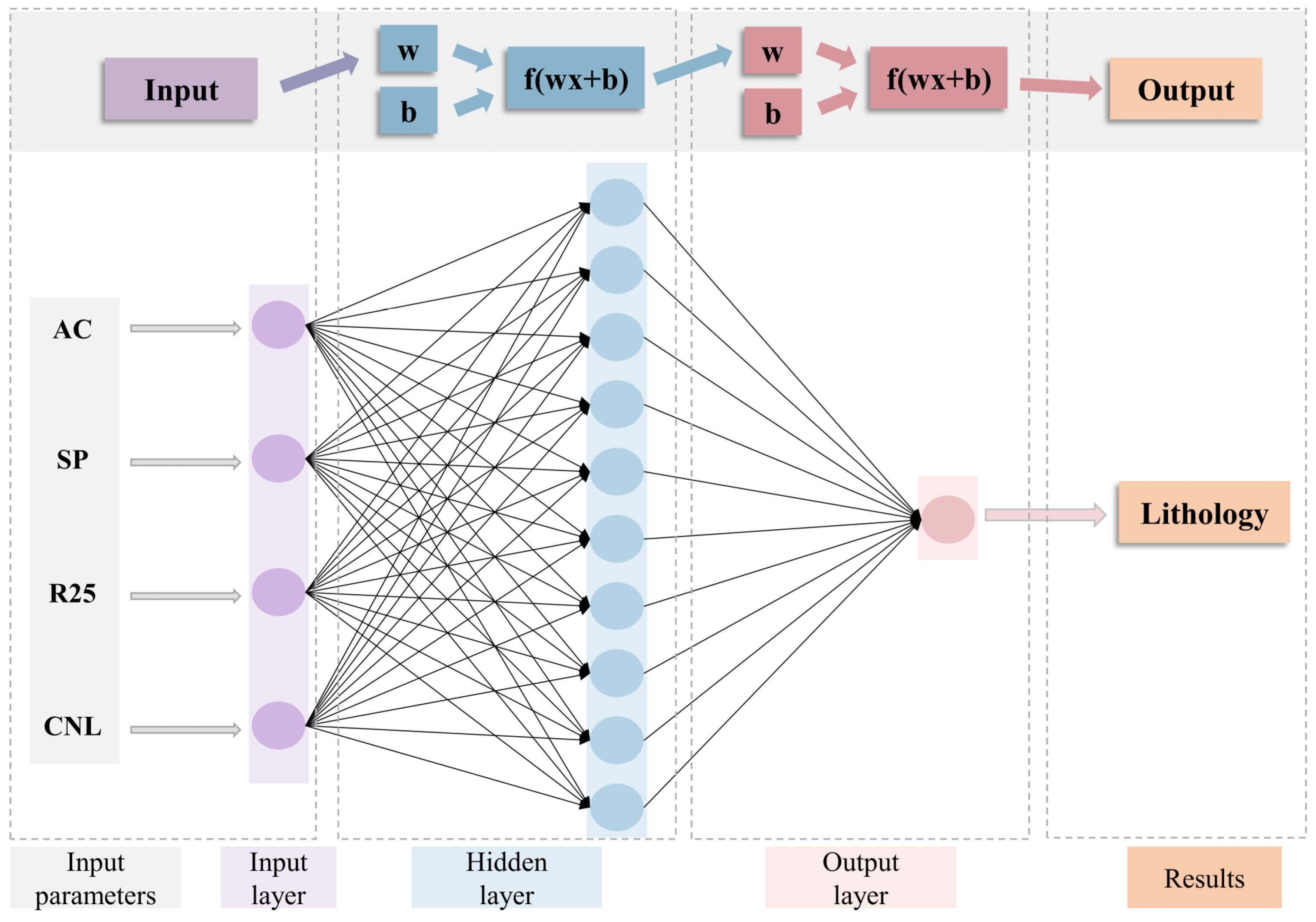
3.3. The BP Neural Network

The BP neural network is a multi-layer feedforward neural network trained by the error backpropagation algorithm, comprising an input layer, output layer, and hidden layer [33]. It has self-learning ability, particularly promotion, generalization, and self-adaptive ability, and is one of the most widely used neural network models [26]. The basic principle of the BP neural network for predicting mineral components is to find a mapping relationship by continuously modifying the network weights and correction threshold until a satisfactory accuracy is obtained [34,35]. The most basic algorithm of the BP neural network is the steepest descent method, including the forward propagation of the signal and the backpropagation of the error.

In the multi-layer forward propagation process, the output formula of each hidden layer unit is as follows:

$$Y_j=f\left({\displaystyle \sum _{i=1}^n(w_{ij}\cdot x_i)+b_j}\right)$$

(9)

where $f=\frac{1}{1+e^{-x}}$ is the activation function, w_ij represents the input weight, b_i represents the offset, x_i represents the output of the input layer, and Y_j represents the output result of the j-th layer.

In the multi-layer forward propagation process, the output formula of each unit of the output layer is as follows:

$$Y_k=f\left({\displaystyle \sum _{i=1}^n(w_{ik}\cdot x_i)+b_k}\right)$$

(10)

where Y_k represents the output result of the output layer, w_jk is the weight from the j-th hidden layer neuron to the k-th output layer neuron, x_j represents the output of the hidden layer, and b_k represents the neuron offset of the hidden layer.

In error backpropagation, the output error signal of each layer of neurons is calculated from the output layer to the input layer. Through the error gradient descent method, the weights and thresholds of each layer are adjusted to minimize the mean square error (MSE). MSE can be expressed as:

$$MSE=\frac{1}{2n}{\displaystyle {\sum }_i^n{E}_i^2}$$

(11)

where E_i is the error of the i-th input data, and n represents the amount of input data.

The adjustment formula of weight is as follows:

$$w_{i(j+1)}=\varphi \cdot {\delta }_j\cdot Y_k\cdot Y_i+a\cdot \mathsf{\Delta }{w}_{ij}$$

(12)

where w_i(j+1) represents the weights from the i-th input layer to the j+1-th hidden layer, ϕ represents the learning step, δ_j represents the error, Y_i represents the result of the input layer, and a represents the momentum factor. Δw_ij is the output result from the i-th input layer to the j-th hidden layer. The momentum factor a is to prevent partial error minimization, using momentum to slide past these minima.

The adjustment formula for the threshold is as follows:

$$b_{j+1}=a\cdot b_j+\varphi \cdot {\delta }_{j+1}$$

(13)

where b_j+1 is the threshold of the j+1-th hidden layer, and b_j represents the threshold of the j-th hidden layer.

AC, SP, CNL, and R25 are used as input parameters. Seven lithologies are coded separately: sandstone is 1, sandy mudstone is 2, mudstone is 3, calcareous mudstone is 4, dolomite is 5, limestone is 6, and shale is 7. A total of 128 sets of data are randomly selected as training samples, and the weights are continuously updated for training to determine the network structure. In this study, the hidden layer contains ten neurons, and the value of the momentum factor is 0.95. The process of identifying lithology based on the BP neural network is shown in Figure 5. The remaining data are used as a test sample to test the model’s accuracy independently.

3.4. The Classification and Regression Tree (C&RT)

C&RT, as a classification model, was proposed by Breiman et al. in 1984 [36], and it is an efficient method for solving classification problems. The branch criterion is the core criterion of decision tree classification, and the change in the branch criterion produces different types of decision trees. The branching criterion of C&RT is established based on the Gini coefficient. The Gini (G) coefficient represents the probability that a randomly selected sample in the sample set is misclassified. It can be expressed as:

$$G(p)=1-{\displaystyle \sum _{k=1}^k{p}_k^2}$$

(14)

where k represents the number of categories, P_k is the frequency with which the k-th class appears in the classification results.

For a given sample set, D, its Gini coefficient is expressed as:

$$G(D)=1-{\displaystyle \sum _{k=1}^k{(\frac{\left|C_k\right|}{\left|D\right|})}^2}$$

(15)

where C_k is the number of samples in D that belong to class k.

When feature A takes the value of a, D is divided into two parts, D₁ and D₂. Under the condition of feature A, the G of D is defined as:

$$G(D,A)=\frac{\left|D_1\right|}{\left|D\right|}G(D_1)+\frac{\left|D_2\right|}{\left|D\right|}G(D_2)$$

(16)

Overfitting is an unavoidable problem of C&RT, and pruning is the primary solution [17,37]. Pruning includes pre-pruning and post-pruning. Pre-pruning means stopping the tree from growing before the decision tree is fully formed. Post-pruning generates an initial decision tree according to the largest scale and prunes layer by layer from bottom to top according to certain rules.

The schematic diagram of C&RT identifying lithology is shown in Figure 6. Log data and lithology data of 147 samples were used as input variables and target parameters, respectively. To prevent overfitting, stopping rule was set, where the minimum number of records in the parent branch is 2%, and the maximum risk difference is 1 and set the depth of the tree to 5. The samples were randomly divided into a training set (131) and a test set (16).

4. Results

The canonical function characteristics of the Es₁^L are shown in

Table 1. Canonical function eigenvalue contribution rate statistics table.

Function	Eigenvalues	Percent Variance (%)	Cumulative Percentage (%)	Canonical Correlation
1	0.731	74.6	74.6	0.65
2	0.178	18.1	92.7	0.388
3	0.054	5.5	98.2	0.226
4	0.018	1.8	100	0.131

. The eigenvalues of function 1 and function 2 are high, and the cumulative contribution rate is 92.7%, which contains most of the lithological information. As a result, function 1 and function 2 are selected as the characteristic variables of lithology discrimination, and the discriminant function of lithology is constructed. The discriminant function is as follows:

$$\{\begin{array}{l}{y}_{sandstone}=198.445\times AC+13.132\times SP+149.108\times R25-30.769\times CNL-89.227\\ y_{sandy,mudstone}=203.262\times AC+3.529\times SP+157.391\times R25-24.92\times CNL-94.781\\ y_{mudstone}=211.363\times AC+11.009\times SP+155.451\times R25-22.273\times CNL-100.783\\ y_{calcareou,smudstone}=222.459\times AC+13.391\times SP+159.739\times R25-24.898\times CNL-110.158\\ y_{dolomite}=213.758\times AC+12.752\times SP+163.179\times R25-25.559\times CNL-107.449\\ y_{limestone}=223.749\times AC+6.023\times SP+151.782\times R25-30.619\times CNL-100.398\\ y_{shale}=225.139\times AC+12.258\times SP+167.792\times R25-25.159\times CNL-114.750\end{array}$$

(17)

The lithology identification results of FDA are shown in the

Table 2. Lithology of samples and results of three methods to predict lithology.

No.	Lithology	FDA	BP Neural Network		C&RT
		Prediction of Lithology	Prediction of Lithology	Sample Type	Prediction of Lithology	Sample Type
1	sandstone	sandstone	sandstone	training	sandstone	training
2	sandstone	sandy mudstone	sandstone	test	sandstone	training
3	sandstone	sandy mudstone	sandstone	training	sandstone	training
4	sandstone	sandstone	sandstone	training	sandstone	training
5	sandstone	sandstone	sandstone	test	sandstone	training
6	sandstone	sandstone	sandstone	training	sandstone	training
7	sandstone	sandstone	sandstone	training	sandstone	training
8	sandstone	sandstone	sandstone	training	sandstone	training
9	sandstone	sandstone	sandstone	training	sandstone	training
10	sandstone	sandstone	sandstone	training	sandstone	training
11	sandstone	sandstone	sandstone	training	sandstone	training
12	sandstone	sandstone	sandstone	training	sandstone	training
13	sandstone	sandstone	dolomite	test	sandstone	training
14	sandstone	sandstone	sandstone	training	sandstone	training
15	sandstone	sandstone	sandstone	test	sandstone	training
16	sandstone	sandstone	sandstone	training	sandstone	training
17	sandstone	sandstone	sandstone	test	sandstone	training
18	sandstone	sandstone	sandstone	training	mudstone	training
19	sandstone	shale	sandstone	training	sandstone	training
20	sandstone	sandstone	sandstone	training	sandstone	training
21	sandstone	shale	sandstone	training	sandstone	test
22	sandstone	sandstone	sandstone	training	sandstone	training
23	sandstone	sandstone	sandstone	training	sandstone	training
24	sandstone	sandstone	sandstone	training	sandstone	training
25	sandstone	sandstone	sandstone	training	sandstone	training
26	sandstone	sandstone	sandstone	training	sandstone	training
27	sandstone	sandstone	sandstone	training	sandstone	training
28	sandstone	sandstone	sandstone	training	sandstone	training
29	sandstone	mudstone	sandstone	training	sandstone	training
30	sandstone	sandstone	sandstone	training	sandstone	training
31	sandstone	sandstone	sandstone	training	sandstone	training
32	sandstone	shale	sandstone	test	sandstone	training
33	sandstone	sandstone	sandstone	training	sandstone	training
34	sandstone	shale	sandstone	training	sandstone	training
35	sandstone	sandstone	sandstone	training	sandstone	training
36	sandstone	sandstone	sandstone	training	sandstone	training
37	sandstone	sandstone	sandstone	training	sandstone	training
38	sandy mudstone	limestone	sandy mudstone	training	sandy mudstone	training
39	sandy mudstone	shale	dolomite	training	dolomite	training
40	sandy mudstone	sandstone	sandy mudstone	training	sandy mudstone	training
41	sandy mudstone	sandy mudstone	sandy mudstone	training	sandstone	training
42	sandy mudstone	sandy mudstone	sandstone	training	sandstone	test
43	sandy mudstone	shale	sandy mudstone	training	sandy mudstone	training
44	mudstone	shale	mudstone	training	mudstone	training
45	mudstone	mudstone	mudstone	training	mudstone	training
46	mudstone	mudstone	mudstone	training	mudstone	training
47	mudstone	mudstone	mudstone	training	mudstone	training
48	mudstone	mudstone	mudstone	training	mudstone	training
49	mudstone	shale	mudstone	test	mudstone	training
50	mudstone	shale	mudstone	training	mudstone	training
51	mudstone	sandstone	mudstone	training	mudstone	training
52	mudstone	sandstone	mudstone	training	sandstone	training
53	mudstone	sandy mudstone	mudstone	test	shale	training
54	mudstone	sandy mudstone	mudstone	training	mudstone	test
55	mudstone	sandy mudstone	sandstone	training	mudstone	training
56	mudstone	sandy mudstone	mudstone	training	mudstone	training
57	mudstone	sandstone	sandstone	training	mudstone	training
58	mudstone	sandstone	mudstone	training	mudstone	training
59	mudstone	shale	shale	training	mudstone	training
60	mudstone	shale	mudstone	training	mudstone	training
61	mudstone	shale	mudstone	training	mudstone	training
62	mudstone	sandstone	mudstone	training	mudstone	training
63	mudstone	shale	mudstone	training	mudstone	training
64	mudstone	shale	Calcareous mudstone	training	mudstone	training
65	mudstone	shale	mudstone	training	sandstone	training
66	mudstone	shale	mudstone	training	mudstone	training
67	mudstone	shale	shale	training	mudstone	training
68	Calcareous mudstone	mudstone	Calcareous mudstone	training	mudstone	training
69	Calcareous mudstone	mudstone	Calcareous mudstone	test	Calcareous mudstone	training
70	Calcareous mudstone	sandstone	Calcareous mudstone	training	Calcareous mudstone	training
71	Calcareous mudstone	shale	shale	training	shale	training
72	Calcareous mudstone	shale	Calcareous mudstone	training	Calcareous mudstone	training
73	Calcareous mudstone	shale	shale	training	Calcareous mudstone	test
74	Calcareous mudstone	shale	sandstone	training	Calcareous mudstone	training
75	Calcareous mudstone	sandstone	sandstone	training	sandstone	training
76	Calcareous mudstone	shale	shale	training	mudstone	training
77	Calcareous mudstone	shale	mudstone	test	Calcareous mudstone	training
78	Calcareous mudstone	shale	mudstone	training	Calcareous mudstone	training
79	Calcareous mudstone	shale	Calcareous mudstone	training	Calcareous mudstone	test
80	dolomite	shale	dolomite	training	dolomite	test
81	dolomite	shale	shale	training	dolomite	training
82	dolomite	shale	shale	training	dolomite	training
83	dolomite	shale	dolomite	training	dolomite	training
84	dolomite	sandstone	dolomite	training	shale	training
85	dolomite	shale	dolomite	training	dolomite	training
86	dolomite	shale	dolomite	training	dolomite	training
87	dolomite	shale	dolomite	test	dolomite	training
88	dolomite	sandstone	dolomite	training	sandstone	training
89	dolomite	sandstone	dolomite	training	dolomite	training
90	dolomite	sandstone	dolomite	training	dolomite	training
91	dolomite	shale	dolomite	training	dolomite	training
92	dolomite	shale	shale	training	shale	test
93	dolomite	shale	dolomite	test	dolomite	training
94	dolomite	shale	dolomite	training	dolomite	training
95	dolomite	shale	shale	training	shale	training
96	dolomite	mudstone	dolomite	training	dolomite	test
97	limestone	sandy mudstone	limestone	training	limestone	training
98	limestone	limestone	limestone	training	shale	training
99	limestone	shale	limestone	training	limestone	training
100	shale	sandstone	Calcareous mudstone	training	shale	training
101	shale	shale	shale	training	shale	training
102	shale	shale	shale	training	shale	training
103	shale	shale	dolomite	training	shale	training
104	shale	shale	shale	test	shale	training
105	shale	shale	shale	training	shale	training
106	shale	shale	shale	training	shale	training
107	shale	shale	shale	test	shale	training
108	shale	shale	dolomite	training	shale	training
109	shale	shale	dolomite	training	dolomite	training
110	shale	shale	shale	test	shale	training
111	shale	shale	shale	training	shale	training
112	shale	shale	shale	training	shale	training
113	shale	shale	shale	training	shale	training
114	shale	shale	shale	training	shale	training
115	shale	shale	shale	training	shale	training
116	shale	shale	dolomite	training	shale	training
117	shale	shale	shale	training	shale	training
118	shale	shale	shale	training	shale	training
119	shale	shale	shale	training	shale	training
120	shale	shale	shale	training	shale	training
121	shale	shale	shale	training	shale	training
122	shale	shale	shale	training	shale	training
123	shale	shale	shale	training	shale	training
124	shale	shale	shale	test	shale	training
125	shale	shale	shale	training	shale	training
126	shale	shale	shale	training	shale	training
127	shale	shale	shale	test	shale	training
128	shale	sandstone	Calcareous mudstone	training	shale	training
129	shale	shale	shale	training	shale	training
130	shale	shale	shale	training	shale	training
131	shale	sandy mudstone	shale	training	shale	training
132	shale	limestone	shale	training	shale	training
133	shale	shale	dolomite	training	shale	training
134	shale	sandy mudstone	shale	training	limestone	training
135	shale	shale	shale	training	mudstone	training
136	shale	shale	shale	training	shale	training
137	shale	shale	shale	training	shale	training
138	shale	shale	shale	training	shale	training
139	shale	shale	shale	training	shale	training
140	shale	shale	shale	training	mudstone	training
141	shale	sandstone	shale	training	shale	training
142	shale	sandstone	shale	training	shale	training
143	shale	shale	shale	training	shale	training
144	shale	shale	shale	test	shale	training
145	shale	shale	shale	training	shale	training
146	shale	shale	shale	training	shale	training
147	shale	sandstone	shale	test	sandstone	training

and Figure 7a, the identification effect of shale and sandstone is good, and the accuracy is 83.3% and 81.1%, respectively. Sandy mudstone and limestone have lower accuracy, both below 50%. The identification of other lithologies is not suitable. Calcareous mudstone and dolomite were not correctly classified. A total of 66.7% of calcareous mudstone and 70.6% of dolomite were wrongly classified as shale. The FDA’s overall accuracy in identifying lithology was 52.4%.

The accuracy rate of the BP neural network in identifying the Es₁^L was 82.3%. The accuracy rate of 19 of these test samples was 89.4%. Limestone and sandstone can be accurately identified by BP neural network with an accuracy of 100% and 97.3%, respectively, and shale, mudstone, and dolomite have an accuracy of 85.4%, 79.2%, and 76.5%, respectively, which can be well-identified. The calcareous mudstone has a poor recognition effect. The calcareous mudstone is wrongly divided into sandstone, mudstone, and shale (Figure 7b).

In the C&RT model, sandstone, shale, mudstone, and dolomite can be well-identified, with an accuracy of more than 75%, and the highest accuracy of sandstone is 97.3% (Figure 7c). Only half of the sandy mudstone is correctly identified, and the wrong part is mainly classified as sandstone. A total of 16 test samples were used, including sandstone, sandy mudstone, mudstone, calcareous mudstone, and dolomite. The CR&T model’s prediction accuracy was 88%. The accuracy rate of the C&RT model in identifying lithology was 85.7%.

5. Discussion

5.1. Logging Characteristics of Lithology

Lithology describes the physical properties of rock, such as color, texture, grain size, and composition [38]. Differences in these physical properties produce different response characteristics in logging, and analyzing these characteristics can invert the distribution of various subsurface lithologies [39,40]. The following is a brief description of the response characteristics of the well logs used in this study:

(1) AC is the recorded time it takes for a sound wave to travel at a fixed interval between formations. The formation contains not only rock but also water, CO₂, CH₄, and hydrocarbon fluids (oil and bitumen) in the pores of the rock [41,42,43,44]. Sound waves travel faster in solids such as rocks and minerals than in other fluids such as water and oil. Even the difference in lithology in the rock affects the propagation velocity of sound waves [10]. The P-wave velocity of mudstone, sandstone, limestone, and dolomite is 1800 m/s, 2130~5180 m/s, 3950~4900 m, 4000~5650 m/s, and 4600~6100 m/s, respectively [45], among which the porosity of sandstone, limestone, and dolomite is between 5% and 20%.

(2) SP represents the natural potential difference between the trajectory of the wellbore and the ground [46]. SP has a good effect in identifying sandstone with developed pores and mudstone. Tight rocks such as calcareous mudstone and shale often have higher electrical resistance than mudstone. However, SP is also affected by the type of reservoir fluid, salinity, and saturation. Using SP to judge lithology often needs to be combined with other logging.

(3) GR is recording the total natural gamma radiation intensity in the rock with a gamma-ray detector [47]. Uranium, thorium, and potassium play a decisive role in natural gamma radioactivity in rocks. Minerals such as gypsum (CaSO₄·H₂O), anhydrite (CaSO₄), quartz (SiO₂), dolomite (CaMgCO₃), and calcite (CaCO₃) in sedimentary rocks have low radioactivity, and with the increase in clay content, the radioactivity becomes stronger. Among the clay minerals, montmorillonite has a large surface area, a strong ability to adsorb radioactive substances, and contains more uranium oxide, which is the main contributor to radioactivity; potassium in illite can also adsorb uranium oxide and is radioactive.

(4) CAL measures the change in borehole diameter with depth, which is related to lithology and the mud used for drilling [48]. The well diameter of sandstone with good permeability is smaller than that of the drill bit. On the contrary, the well diameter of easily collapsed mudstone and carbonate rock with developed pores is larger than the drill bit. Lithology is classified based on these features. As a result, the change in well diameter is also related to cementing quality and wellbore azimuth, and lithology identification needs to be combined with other well logs.

(5) In general, sandstone with high resistance is sandstone, mudstone with low resistance, and reservoirs containing fluids are also low resistivity. However, many factors affect resistivities, such as mud invasion, electrode spacing, and wellbore inclination [49]. Therefore, it is mainly used for qualitative analysis, and further analysis needs to be combined with other data.

(6) CNL measures the amount of hydrogen because hydrogen slows down high-energy and fast neutrons [46]. Sandstone, dolomite, limestone, and migmatites are commonly found in reservoirs. The minerals that make up these rocks have no hydrogen, and most of the hydrogen is in the fluids in the pores of the rocks. Among them, the deceleration capacity of saturated freshwater sandstone is less than that of limestone, and the deceleration capacity of saturated freshwater limestone is lower than that of dolomite [9]. The pores of mudstone and shale contain bound water, and clay minerals contain crystal water. The higher the clay content, the higher the hydrogen content.

(7) DEN irradiates the formation with gamma rays and measures the bulk density of the formation according to the Compton effect [47]. The density of a liquid is much lower than that of solid minerals. The densities of several common minerals are quartz (2.65 g/cm³), calcite (2.71 g/cm³), dolomite (2.87 g/cm³), gypsum (2.32 g/cm³), and anhydrite (2.96 g/cm³). The reference densities of the corresponding rocks for these minerals are sandstone (2.644 g/cm³), limestone (2.710 g/cm³), dolomite (2.877 g/cm³), gypsum (2.355 g/cm³), and anhydrite (2.960 g/cm³). The porosity of these rocks is close to zero.

The logging characteristics of the lithology described above are ideal, but the actual formation is often more complex. In particular, the continental lake basins are affected by severe sedimentation and diagenesis, with strong inorganic heterogeneity [26,50], mostly mixed rocks, and blurred lithologic boundaries. Mudstone and shale strata are widely developed in the Es₁^L, mainly mudstone and shale, with dolomite, limestone, sandstone, and migmatite interlayers. Therefore, the rock density, radioactive element content, and well diameter of the whole section have little change. Combined with mathematical analysis, AC, SP, CNL, and R25 were selected as input parameters. The direct relationship between the four logging curves is poor, and the lithology is not classified on the intersection of the four logging curves (Figure 8). Clay minerals are rich in crystalline water, adsorbed water, and oil in the pores of mudstone [51], and mudstone has a high CNL value. Shale, calcareous mudstone, and some mudstones have a high degree of overlap, and the mineral compositions of the three are similar and difficult to distinguish. Effective identification of complex lithologies is therefore required with the help of some other measures.

5.2. Comparison of the Three Models

Table 2 shows the differences in the prediction results of the three methods. Shale and sandstone can be accurately identified by FDA, BP neural network, and C&RT, and the identification accuracy is above 80% (Figure 7). Sandy mudstone and calcareous mudstone are mixed rocks with poor recognition effects. C&RT has the highest accuracy in identifying sandy mudstone and calcareous mudstone, with 50.0% and 66.7% accuracy rates, respectively (Figure 7). BP neural network and C&RT have the same results in identifying dolomite, while FDA cannot identify dolomite. The lithology recognition accuracies of FDA, BP neural network, and C&RT models are 52.4%, 82.3%, and 85.7%, respectively (Figure 7). FDA cannot be effectively applied to the identification of complex lithology. The complicated lithology of continental shale formations can be more accurately identified by BP neural network and C&RT; however, BP neural network is a “black box” and cannot be seen. This issue can be solved more effectively with C&RT since each step of the identification process can be presented and adjusted to the demands. C&RT is a lithology identification method therefore suitable to the Es₁^L.

5.3. Application

Well B11x is located in the Xiliu area of Raoyang sag. It is a typical shale oil exploration well in Raoyang sag. Using the established BP neural network and C&RT model to identify lithology, the lithology distribution characteristics of the Es₁^L of well B11x were analyzed. The Es₁^L of well B11x is dominated by mudstone and shale, with interlayers of calcareous mudstone, sandstone, and dolomite. The core lithology in Figure 9 is obtained from mud logging data. These data are greatly influenced by artificial subjective, especially in the continental shale strata with heterogeneity and strength, and the accuracy of the data remains to be discussed. Nonetheless, it can also be used as a reference point to advise on some geological work. The lithological identification results of the BP neural network show that sandstone can be effectively identified. However, shale, mudstone, calcareous mudstone, and dolomite with similar mineral compositions cannot be distinguished. At 3512.91~3513.13 m, the rock core shows mudstone, while the prediction result of the BP neural network is shale. The bedding fractures of shale have larger storage space [52], which reduces the value of AC. The natural potential of this section does not change much, and the value of AC is high. Combined with the photos of the rock core (Figure 10), the rock of this section is mudstone. Figure 10b shows that the upper bedding at 3547.90~3548.06 m is developed as shale, and the lower part is dolomite. At 3564.06~3564.36 m, the rock has a blocky structure without bedding.

The recognition result of C&RT is better than that of the BP neural network, especially in the recognition of interlayers and thin interlayers, which are usually favorable intervals for the exploration and development of shale oil. The lithology identified by C&RT is highly similar to the lithology obtained from mud logging, but there are also differences. For example, at 3509.37~3509.63 m, the core lithology shows calcareous mudstone, while the thin section identification result is shale, and the recognition result of C&RT is the same. The acoustic transit time of this section is small, the resistivity is low, and the value of CNL is high, indicating that it has a larger storage space and more water. This response is usually due to interlayer fractures in the shale in tight reservoirs. The acoustic time difference of carbonate rocks is higher than that of tight shale. Carbonate rocks can form reservoir spaces containing fluids due to dissolution [53]. Fluids and primary spaces increase the hydrogen content and reduce resistivity. At 3547.90~3548.06m, the values of AC and CNL are high, and the resistivity is low. Combined with thin section identification, the lithology is dolomite.

The accuracy of the BP neural network identification lithology model is lower than that of the C&RT model in identifying mixed lithology. Although the accuracy of the two models differs by only 3.4%, it can be found in the process of model application that identifying each lithology by C&RT is reasonable. Therefore, it is practical to use C&RT to identify lithology, and it can provide a reference for the exploration and development of shale oil in shale intervals.

6. Conclusions

The identification of complex lithology is a typical nonlinear classification problem. Intelligent algorithms can effectively solve this problem. Different algorithms have different identification effects on different lithologies. Through FDA, BP neural network, and C&RT to identify the complex lithology of the mudstone and shale strata in the Es₁^L of Raoyang Sag, the following conclusions are drawn:

(1) Each logging has a different sensitivity to lithology. The four logs AC, SP, CNL, and R25 of the Es₁^L the Raoyang sag have the highest sensitivity to seven lithologies and are used as input parameters for lithology identification.

(2) The intersection graph method cannot distinguish complex lithology. FDA, BP neural network, and C&RT have an accuracy of 52.4%, 82.3%, and 85.7%, respectively, in identifying the Es₁^L. The accuracy of the BP neural network in identifying mixed lithology is lower than that of C&RT, and the accuracy of C&RT in identifying sandstone, shale, and mudstone is 97.3%, 89.6%, and 87.5%, respectively.

(3) C&RT can identify interlayers and thin interlayers in shale strata. The C&RT identification results of well B11x show that the lithology is dominated by shale, with mudstone, sandstone, calcareous mudstone, and dolomite interlayers.

References

1. Selley, R.C. An Introduction to Sedimentology; Academic Press: London, UK, 1976. [Google Scholar]
2. Tian, M.; More, H.; Xu, H. Inversion of well logs into lithology classes accounting for spatial dependencies by using hidden markov models and recurrent neural networks. J. Petrol. Sci. Eng. 2021, 196, 107598. [Google Scholar] [CrossRef]
3. Li, Z.; Kang, Y.; Feng, D.; Wang, X.-M.; Lv, W.; Chang, J.; Zheng, W.X. Semi-supervised learning for lithology identification using Laplacian support vector machine. J. Petrol. Sci. Eng. 2020, 195, 107510. [Google Scholar] [CrossRef]
4. Burke, J.A.; Campbell, R.L.; Schmidt, A.W. The litho-porosity cross plot a method of determining rock characteristics for computation of log data. In Proceedings of the SPE Illinois Basin Regional Meeting, Evansville, IN, USA, 30–31 October 1969. [Google Scholar]
5. Busch, J.M.; Fortney, W.G.; Berry, L.N. Determination of lithology from well logs by statistical analysis. Spe Form. Eval. 1987, 2, 412–418. [Google Scholar] [CrossRef]
6. Liu, A.; Zuo, L.; Li, J.; Li, R.; Zhang, R. Application of principal component analysis in carbon ate lithology identification: A case study of the Cambrian carbonate reservoir in YH field. Oil Gas Geol. 2013, 34, 192. [Google Scholar]
7. Xie, Y.; Zhu, C.; Zhou, W.; Li, Z.; Liu, X.; Tu, M. Evaluation of machine learning methods for formation lithology identification: A comparison of tuning processes and model performances. J. Petrol. Sci. Eng. 2018, 160, 182–193. [Google Scholar] [CrossRef]
8. Jiang, Z.; Liang, C.; Wu, J.; Zhang, J.; Zhang, W.; Wang, Y.; Liu, H.; Chen, X. Several issues in sedimentological studies on hydrocarbon-bearing fine-grained sedimentary rocks. Acta Petrol. Sin. 2013, 34, 1031–1039. [Google Scholar]
9. Carrasquilla, A.; Lima, R. Basic and specialized geophysical well logs to characterize an offshore carbonate reservoir in the Campos Basin, southeast Brazil. J. S. Am. Earth. Sci. 2020, 98, 102436. [Google Scholar] [CrossRef]
10. Dong, S.; Zeng, L.; Du, X.; He, J.; Sun, F. Lithofacies identification in carbonate reservoirs by multiple kernel Fisher discriminant analysis using conventional well logs: A case study in A oilfield, Zagros Basin, Iraq. J. Petrol. Sci. Eng. 2021, 210, 110081. [Google Scholar] [CrossRef]
11. Sebtosheikh, M.A.; Salehi, A. Lithology prediction by support vector classifiers using inverted seismic attributes data and petrophysical logs as a new approach and investigation of training data set size effect on its performance in a heterogeneous carbonate reservoir. J. Petrol. Sci. Eng. 2015, 134, 143–149. [Google Scholar] [CrossRef]
12. Bhattacharya, S.; Carr, T.R.; Pal, M. Comparison of supervised and unsupervised approaches for mudstone lithofacies classification: Case studies from the Bakken and Mahantango-Marcellus Shale, USA. J. Nat. Gas Sci. Eng. 2016, 33, 1119–1133. [Google Scholar] [CrossRef]
13. Deng, C.; Pan, H.; Fang, S.; Konaté, A.A.; Qin, R. Support vector machine as an alternative method for lithology classification of crystalline rocks. J. Geophys. Eng. 2017, 14, 341–349. [Google Scholar] [CrossRef]
14. Sun, J.; Li, Q.; Chen, M.; Ren, L.; Huang, G.; Li, C.; Zhang, Z. Optimization of models for a rapid identification of lithology while drilling—A win-win strategy based on machine learning. J. Petrol. Sci. Eng. 2019, 176, 321–341. [Google Scholar] [CrossRef]
15. Merembayev, T.; Yunussov, R.; Yedilkhan, A. Machine learning algorithms for classification geology data from well logging. In Proceedings of the International Conference on Electronics Computer and Computation, Kaskelen, Kazakhstan, 29 November–1 December 2018. [Google Scholar]
16. Dev, V.A.; Eden, M.R. Evaluating the Boosting Approach to Machine Learning for Formation Lithology Classification. Comput. Chem. Eng. 2018, 44, 1465–1470. [Google Scholar] [CrossRef]
17. Saporetti, C.M.; da Fonseca, L.G.; Pereira, E.; de Oliveira, L.C. Machine learning approaches for petrographic classification of carbonate-siliciclastic rocks using well logs and textural information. J. Appl. Geophys. 2018, 155, 217–225. [Google Scholar] [CrossRef]
18. Yang, H.; Pan, H.; Ma, H.; Konaté, A.A.; Yao, J.; Guo, B. Performance of the synergetic wavelet transform and modified K-means clustering in lithology classification using nuclear log. J. Petrol. Sci. Eng. 2016, 144, 1–9. [Google Scholar] [CrossRef]
19. Raeesi, M.; Moradzadeh, A.; Doulati Ardejani, F.; Rahimi, M. Classification and identification of hydrocarbon reservoir lithofacies and their heterogeneity using seismic attributes, logs data and artificial neural networks. J. Petrol. Sci. Eng. 2012, 82–83, 151–165. [Google Scholar] [CrossRef]
20. Zych, M.; Stachura, G.; Hanus, R.; Szabó, N.P. Application of Artificial Neural Networks in Identification of Geological Formations on the Basis of Well Logging Data—A Comparison of Computational Environments’ Efficiency. In International Seminar of Metrology Methods and Techniques of Signal Processing in Physical Measurements; Springer: Rzeszow, Poland, 2018. [Google Scholar]
21. Maia Ramos Lopes, D.; Neves Andrade, A.J. Lithology identification on well logs by fuzzy inference. J. Petrol. Sci. Eng. 2019, 180, 357–368. [Google Scholar] [CrossRef]
22. Li, S.; Zhou, K.; Zhao, L.; Xu, Q.; Liu, J. An improved lithology identification approach based on representation enhancement by logging feature decomposition, selection and transformation. J. Petrol. Sci. Eng. 2021, 209, 109842. [Google Scholar] [CrossRef]
23. Ren, Q.; Zhang, H.; Zhang, D.; Zhao, X.; Yan, L.; Rui, J. A novel hybrid method of lithology identification based on k-means++ algorithm and fuzzy decision tree. J. Petrol. Sci. Eng. 2022, 208, 109681. [Google Scholar] [CrossRef]
24. Gardner, M.W.; Dorling, S.R. Artificial neural networks (the multilayer perceptron)—A review of applications in the atmospheric sciences. Atmos. Environ. 1998, 32, 2627–2636. [Google Scholar] [CrossRef]
25. Dong, S.; Wang, Z.; Zeng, L. Lithology identification using kernel Fisher discriminant analysis with well logs. J. Petrol. Sci. Eng. 2016, 143, 95–102. [Google Scholar] [CrossRef]
26. Song, Z.; Li, J.; Li, X.; Chen, K.; Wang, C.; Li, P.; Wei, Y.; Zhao, R.; Wang, X.; Zhang, S.; et al. Coupling Relationship between Lithofacies and Brittleness of the Shale Oil Reservoir: A Case Study of the Shahejie Formation in the Raoyang Sag. Geofluids 2022, 2022, 2729597. [Google Scholar] [CrossRef]
27. Wei, Y.; Li, X.; Zhang, R.; Li, X.; Lu, S.; Qiu, Y.; Jiang, T.; Gao, Y.; Zhao, T.; Songm, Z.; et al. Influence of a Paleosedimentary Environment on Shale Oil Enrichment: A Case Study on the Shahejie Formation of Raoyang Sag, Bohai Bay Basin, China. Front. Earth Sci.-Prc. 2021, 9, 736054. [Google Scholar] [CrossRef]
28. Li, X.; Chen, K.; Li, P.; Li, J.; Geng, H.; Li, B.; Li, X.; Wang, H.; Zhang, L.; Wei, Y.; et al. A New Evaluation Method of Shale Oil Sweet Spots in Chinese Lacustrine Basin and Its Application. Energies 2021, 14, 5519. [Google Scholar] [CrossRef]
29. Aghli, G.; Soleimani, B.; Moussavi-Harami, R.; Mohammadian, R. Fractured zones detection using conventional petrophysical logs by differentiation method and its correlation with image logs. J. Petrol. Sci. Eng. 2016, 142, 152–162. [Google Scholar] [CrossRef]
30. Asante-Okyere, S.; Shen, C.; Yao, Y.Z.; Rulegeya, M.M.; Zhu, X. A novel hybrid technique of integrating gradient-boosted machine and clustering algorithms for lithology classification. Nat. Resour. Res. 2020, 29, 2257–2273. [Google Scholar] [CrossRef]
31. Duda, R.O.; Hart, P.E.; Stork, D.G. Pattern Classification; John Wiley & Sons: New York, NY, USA, 2001. [Google Scholar]
32. Subasi, A.; Gursoy, M.I. EEG signal classification using PCA, ICA, LDA and support vector machines. Expert Syst. Appl. 2010, 37, 8659–8666. [Google Scholar] [CrossRef]
33. Hornik, K.; Stinchcombe, M.; White, H. Multilayer feedforward networks are universal approximators. Neural Netw. 1989, 2, 359–366. [Google Scholar] [CrossRef]
34. Wu, D.; Zhang, D.; Liu, S.; Jin, Z.; Chowwanonthapunya, T.; Gao, J.; Li, X. Prediction of polycarbonate degradation in natural atmospheric environment of China based on BP-ANN model with screened environmental factors. Chem. Eng. J. 2020, 399, 125878. [Google Scholar] [CrossRef]
35. Jawad, J.; Hawari, A.H.; Zaidi, S.J. Artificial neural network modeling of wastewater treatment and desalination using membrane processes: A review. Chem. Eng. J. 2021, 419, 129540. [Google Scholar] [CrossRef]
36. Lewis, R.J. An introduction to classification and regression tree (CART) analysis. In Proceedings of the Annual Meeting of the Society for Academic Emergency Medicine, San Francisco, CA, USA, 22–25 May 2000. [Google Scholar]
37. Shi, N.; Li, H.; Luo, W. Data mining and well logging interpretation: Application to a conglomerate reservoir. Appl. Geophys. 2015, 12, 263–272. [Google Scholar] [CrossRef]
38. Haldar, S.K. Introduction to Mineralogy and Petrology; Elsevier: Amsterdam, The Netherlands, 2020. [Google Scholar]
39. Zhou, Z.; Wang, G.; Ran, Y.; Lai, J.; Cui, Y.; Zhao, X. A logging identification method of tight oil reservoir lithology and lithofacies: A case from Chang7 Member of Triassic Yanchang Formation in Heshui area, Ordos Basin, NW China. Petrol. Explor. Dev. 2016, 43, 65–73. [Google Scholar] [CrossRef]
40. Liu, G.; Liu, B.; Huang, Z.; Chen, Z.; Jiang, Z.; Guo, X.; Li, T.; Chen, L. Hydrocarbon distribution pattern and logging identification in lacustrine fine-grained sedimentary rocks of the Permian Lucaogou Formation from the Santanghu basin. Fuel 2018, 222, 207–231. [Google Scholar] [CrossRef]
41. Li, J.; Lu, S.; Xie, L.; Zhang, J.; Xue, H.; Zhang, P.; Tian, S. Modeling of hydrocarbon adsorption on continental oil shale: A case study on n-alkane. Fuel 2017, 206, 603–613. [Google Scholar] [CrossRef]
42. Li, J.; Lu, S.; Cai, J.; Zhang, P.; Xue, H.; Zhao, X. Adsorbed and free oil in lacustrine nanoporous shale: A theoretical model and a case study. Energy Fuel 2018, 32, 12247–12258. [Google Scholar] [CrossRef]
43. Li, J.; Lu, S.; Zhang, P.; Cai, J.; Li, W.; Wang, S.; Feng, W. Estimation of gas-in-place content in coal and shale reservoirs: A process analysis method and its preliminary application. Fuel 2020, 259, 116266. [Google Scholar] [CrossRef]
44. Li, W.; Lu, S.; Li, J.; Zhang, P.; Wang, S.; Feng, W.; Wei, Y. Carbon isotope fractionation during shale gas transport: Mechanism, characterization and significance. Sci. China Earth Sci. 2020, 63, 674–689. [Google Scholar] [CrossRef]
45. Cannon, S. Petrophysics: A Practical Guide; John Wiley & Sons: Hoboken, NJ, USA, 2015. [Google Scholar]
46. Lyu, W.; Zeng, L.; Liu, Z.; Liu, G.; Zu, K. Fracture responses of conventional logs in tight-oil sandstones: A case study of the Upper Triassic Yanchang Formation in southwest Ordos Basin, China. AAPG Bulletin. 2016, 100, 1399–1417. [Google Scholar] [CrossRef]
47. Tokhmchi, B.; Memarian, H.; Rezaee, M.R. Estimation of the fracture density in fractured zones using petrophysical logs. J. Petrol. Sci. Eng. 2010, 72, 206–213. [Google Scholar] [CrossRef]
48. Zazoun, R.S. Fracture density estimation from core and conventional well logs data using artificial neural networks: The Cambro-Ordovician reservoir of Mesdar oil field, Algeria. J. Afr. Earth Sci. 2013, 83, 55–73. [Google Scholar] [CrossRef]
49. Shazly, T.F.; Tarabees, E. Using of Dual Laterolog to detect fracture parameters for Nubia Sandstone Formation in Rudeis-Sidri area, Gulf of Suez, Egypt. Egypt. J. Pet. 2013, 22, 313–319. [Google Scholar] [CrossRef]
50. Zhang, X.; Pang, X.; Jin, Z.; Hu, T.; Toyin, A.; Wang, K. Depositional model for mixed carbonate-clastic sediments in the Middle Cambrian Lower Zhangxia Formation, Xiaweidian, North China. Adv. Geo-Energy Res. 2020, 4, 29–42. [Google Scholar] [CrossRef] [Green Version]
51. Li, J.; Wang, S.; Lu, S.; Zhang, P.; Cai, J.; Zhao, J.; Li, W. Microdistribution and mobility of water in gas shale: A theoretical and experimental study. Mar. Petrol. Geol. 2019, 102, 496–507. [Google Scholar] [CrossRef]
52. Sun, Y.; Ju, Y.; Zhou, W.; Qiao, P.; Tao, L.; Xiao, L. Nanoscale pore and crack evolution in shear thin layers of shales and the shale gas reservoir effect. Adv. Geo-Energy Res. 2022, 6, 221–229. [Google Scholar] [CrossRef]
53. Guan, M.; Wu, S.; Hou, L.; Jiang, X.; Ba, D.; Hua, G. Paleoenvironment and chemostratigraphy heterogenity of the Cretaceous organic-rich shales. Adv. Geo-Energy Res. 2021, 5, 444–455. [Google Scholar] [CrossRef]
Figure 1. (a) Map showing the structural characteristic within and surround the Raoyang sag and distribution of sampling wells. (b) Stratigraphic column of the Shahejie Formation (modified after Wei et al., 2021 [27]).
Energies 16 01748 g001
Figure 2. (a,b): sandstone, well G103, 2479.80 m, the mineral composition is dominated by quartz and feldspar; (c,d): sandy mudstone, well N92x, 3276.00 m, silty quartz and feldspar particles are unevenly distributed; (e,f): mudstone, well G34, 2517.56 m, clay structure, the main component is fine scaly clay minerals; (g,h): calcareous mudstone, well Q46, 2860.10 m, the main component is dolomite, a small amount of terrestrial quartz and feldspar, bright crystal dolomite filling between sand debris; (i,j): dolomite, well N202, 3565.26 m, the main component is dolomite, and a small amount of terrigenous fine-grained quartz and feldspar are unevenly distributed; (k,l): limestone, well XL25x, 3550.36 m; (m,n): shale, well B11x, 3543.90 m, development of page bedding structure; (o,p): shale, well G24, 2617.00 m, fine scaly clay minerals, silty quartz, feldspar and iron bands are interbedded with unequal thickness.
Energies 16 01748 g002
Figure 3. Correlation characteristics of conventional logging curves.
Energies 16 01748 g003
Figure 4. Diagram of the FDA.
Energies 16 01748 g004
Figure 5. Schematic diagram of the principle of lithology recognition by BP neural network.
Energies 16 01748 g005
Figure 6. Schematic diagram of C&RT to identify lithology.
Energies 16 01748 g006
Figure 7. Confusion matrix of three lithology identification models.
Energies 16 01748 g007
Figure 8. Cross plots of well logs against lithology labels.
Energies 16 01748 g008
Figure 9. Lithology identification of well B11x by BP neural network and C&RT.
Energies 16 01748 g009
Figure 10. Rock core of well B11x. (a) At 3512.91~3513.13 m, the rock core shows mudstone; (b) The upper bedding at 3547.90~3548.06 m is developed as shale, and the lower part is dolomite; (c) At 3564.06~3564.36 m, the rock has a blocky structure without bedding.
Energies 16 01748 g010