Open-Circuit Fault Detection and Location in AC-DC-AC Converters Based on Entropy Analysis

Abstract

Inverters and converters contain more and more power electronics switches which may subsequently affect their reliability. Therefore, fault detection and location are essential to improve their reliability and to ensure continuous operation. In this paper, an $AC-DC-AC$ converter with three-phase inverter is investigated under permanent, single and multiple open-circuit fault scenarios. Many entropies and multiscale entropies are then proposed to evaluate the complexity of the output currents by quantifying their entropies over a range of temporal scales. Among the multitude of entropies, only some entropies are able to differentiate healthy from open-circuit faulty conditions. Moreover, the simulation results show that these entropies are able to detect and locate the arms of the bridge with open-circuit faults.

1. Introduction

Recently, with the rapid development of power electronics technologies, numerous studies have been conducted on multilevel inverters [1,2] used in various engineering fields [3,4], such as high-power transmission in grids [5], motor drives [6,7] and energy storage devices [3]. Multilevel inverters have become popular because of the improvement in output voltage quality, reduction in switching frequency and the extensibility of the structure. However, the main drawbacks are the higher number of components compared to classical inverters and more complex control.

The safety of power electronics switches is one of the most important issues in the normal operation of inverters. Several researchers have studied the behavior of inverters with internal failure, focusing particularly on the open-circuit fault of a switch. Short-circuit and open-circuit are the most common faults in power switches. Furthermore, short-circuits need to be detected to avoid destructive overcurrents, e.g., using a dedicated gate drive protection hardware circuit [8]. An open-circuit does not necessarily cause system shutdown and can remain undetected for an extended period of time. If an internal fault occurs in the inverter, serious distortion to the voltage and current could result. This may lead to secondary faults in the remaining drive components, resulting in high repair costs.

Open-circuit fault diagnosis methods can be classified as voltage-based or current-based. The former extracts diagnostic features by additional voltage sensors or electrical circuits. The diagnosis strategy presented in [9] is based on pole voltage estimation, requiring knowledge of the line parameters. Through voltage analysis, on the inverter side, it is also possible to detect fault occurrence [8,10]. Under open-circuit faults, these voltages show some characteristic irregularities that can be detected, which enable direct localization of the faulty device. Recently, many current-based, fault diagnosis methods have attracted much attention [5,11,12]. The authors of [13] present an effective open-circuit fault diagnosis approach based on the brushless motor characteristics, observing phase currents and other parameters. The fault diagnosis strategy proposed in [11] is based on an analysis of current waveforms—it identifies the faulty half-leg, but cannot identify the faulty component. In order to improve the diagnosis speed, in [5,12] a current-based diagnosis algorithm is proposed that identifies the reference current errors and their average absolute values. Open-circuit fault detection is of critical importance for the stable operation of inverters. Recently, several fault detection approaches have been developed for power inverters and are discussed below.

Fault detection and location methods are hardware-based or software-based methods: the hardware-based methods require additional sensors, making fault detection complex and costly, whereas software-based methods do not require extra hardware.

There are many fault detection approaches for multi-level converters, including comparison between measured and reference values, the sliding mode observer [14], Lyapunov theory [15], the Kalman filter algorithm [16,17], Fourier transform [18], Park transformation [19], wavelet transform [20], machine learning [21], neural network approaches [22], and the Filippov method [23].

In [5], a diagnosis method for a two-level voltage source inverter based on the average absolute value of current is proposed. The detection of several kinds of faults can be completed using the ratio of the theoretical and the practical voltage values on the capacitor of each inverter’s sub-module [24]. The authors of [14] proposed a sliding mode observer to diagnose any open-circuit fault of the switch and to avoid interference caused by sampling error and system fluctuation. The authors of [16] proposed a Kalman-filter-based approach: the comparison of measured and estimated voltages and currents obtained by the Kalman filter enables detection of the open-circuit fault of a modular multilevel converter sub-module. The amplitude and argument of each phase current harmonic can be used to detect and localize the faults.

An analysis of the first harmonics in [18] showed that the difference between the healthy state and the open-circuit fault case lay in the zero-order harmonic, i.e., the presence of a $DC$ component in the signal. The argument of the zero harmonic with respect to the fundamental enables determination of the type of fault.

The authors of [19,25] proposed a Park technique followed by the polarity of the trajectory slope in the complex $\alpha$-$\beta$ frame to identify the faulty switch. A neural network [22], a mixed kernel support tensor machine [21], an adaptive one-convolutional neural network, or an adaptive linear neural-recursive least squares algorithm, have been utilized to detect and identify faulty switches for multilevel inverters. These strategies can be applied directly to the voltage and current data. However, a large amount of reliable data is required to train the neural network in advance. Fault diagnosis methods are mainly machine-learning based. In [26], an “optimized support vector machine method” is proposed: the fault characteristics are deduced from the average value of the three-phase currents. In [27], wavelet analysis and an improved neural network are used. The authors of [28] use the wavelet energy spectrum entropy to perform a statistical analysis of the energy distribution of the signal in each frequency band. Finally, ref. [29] employed “weighted-amplitude permutation” entropy, with better feature extraction than standard permutation entropy.

Our goal herein is to study the output current of an $AC-DC-AC$ converter using the usual and multiscale entropies, and to evaluate their ability to differentiate a healthy state from an open-circuit faulty state. We are able to pick up the entropies which detect and locate the arm of the bridge with an open-circuit fault. We first present the usual entropies and multiscale entropies and describe the commonly used entropy algorithms. Section 4 presents the dataset we used for the three-phase output currents of the inverter under a healthy state, with one and two open-circuit faults. Then, in Section 5, the results are detailed and discussed, including evaluation of the entropy with variation in the data length, embedding dimension, time lag and tolerance. We end with conclusions in Section 6.

2. Entropy Methods

Serving as an algebraic quantification parameter of time series, the entropy measures the system’s complexity, including the degree of irregularity of time series, to evaluate the probability of finding m-similar patterns. A number of methods to quantify the entropy of a data series have been proposed in recent decades. They aim for higher discriminating power, less noise and parameter dependence. Since the introduction of approximate entropy—$ApEntropy$ [30], other methods have been proposed, such as $SampEntropy$—sample entropy [30], $K2Entropy$—Kolmogorov entropy [31], $CondEntropy$—conditional entropy [32], $CoSiEntropy$—cosine similarity entropy [33], $FuzzEntropy$—fuzzy entropy [33,34,35], $En$$\mathit{of}$$Entropy$—entropy of entropy [36], $MSEntropy$—multiscale entropy functions [37,38,39,40,41], $rMSEntropy$—refined multiscale entropy [42,43], and $cMSEntropy$—composite multiscale entropy [44,45].

• $ApEntropy$ and $SampEntropy$: approximate entropy was proposed by Pincus in 1991. The objective of $ApEntropy$ is to determine how often different patterns of data are found in the dataset. According to [30], the bias of $ApEntropy$ means that the results suggest more regularity than there is in reality. This bias is obviously more important for samples with a small length of the series. Eliminating this bias by preventing each vector from being counted with itself would make $ApEntropy$ unstable in many situations, leaving it undetermined if each vector does not find at least one match. To avoid those two problems, Richman [30] defined $SampEn$, a statistic which does not have self-counting. For a time series ${\left\{x_i\right\}}_{i=1}^N$ with a given embedding dimension m, tolerance r and time lag $\tau$, the Algorithm 1 for determining the $ApEntropy$ of a sequence is as follows:

Algorithm 1: Approximation Entropy

(a) Construct the embedding vectors $x_i^m$ = $[x_i,x_{i+\tau },...,x_{i+(m-1)\tau }].$ (b) Compute the Chebyshev distance                   $ChebDis{t}_{i,j}^m=ma{x}_{k=\overline{1,m}}\left\{\right|x_i^m\left[k\right]-x_j^m\left[k\right]\left|\right\}$. (c) Construct the number of similar patterns $P_i^m\left(r\right)$, when $ChebDis{t}_{i,j}^m\le r$. (d) Compute the local probability of occurrences of similar patterns                               $B_i^m\left(r\right)=\frac{1}{N-m+1}{P}_i^m\left(r\right)$. (e) Compute the global probability of occurrences of similar patterns                               $B^m\left(r\right)=\frac{1}{N-m+1}{\sum }_{i=1}^{N-m+1}{B}_i^m\left(r\right)$. (f) Compute $B^{m+1}\left(r\right)=\frac{1}{N-m}{\sum }_{i=1}^{N-m}{B}_i^{m+1}\left(r\right)$ for the vector $m+1$. (g) Obtain approximation entropy $ApEntropy(m,\tau ,r,N)=ln\frac{B^m\left(r\right)}{B^{m+1}\left(r\right)}$.

• $K2Entropy$: certain information provided by times series can only be extracted by analyzing the dynamical characteristics. The conventional entropy gives information about the number of states available for the dynamical system in phase space. Therefore, it does not provide any information on how the system evolves. On the contrary, the $K2Entropy$ [31] takes into account how often these states are visited by a trajectory, i.e., it provides information about the dynamic evolution of the system.
  The initial time series ${\left\{x_i\right\}}_{i=1}^N$ can be divided into a finite partition $\alpha =\{C_1,C_2,...,C_k\}$, according to $C_k=[x\left(i\tau \right),x\left((i+1)\tau \right),...,x\left((i+k-1)\tau \right)]$, where $\tau$ is the time delay parameter. The Shannon entropy of such a partition is given as:

  $$K(\tau ,k)=-\sum _{C\in \alpha }p\left(C\right)·logp\left(C\right).$$

  (1)
  The Kolmogorov entropy [31] is then defined by

  $$K2Entropy=-\underset{\alpha finitepartition}{sup}\underset{N\to \infty }{lim}\frac{1}{N}\sum _{n=0}^{N-1}(K_{n+1}(\tau ,k)-K_n(\tau ,k)).$$

  (2)
  The difference $K_{n+1}(\tau ,k)-K_n(\tau ,k)$ is the average information needed to predict which partition will be visited.
• $CondEntropy$: Porta [32] reports the conditional entropy ($CondEntropy$) to distinguish the entropy variation over short data sequences. A time series ${\left\{x_i\right\}}_{i=1}^N$ is reduced to a process with zero mean and unitary variance by means of the normalisation

  $$x\left(i\right)=\frac{X\left(i\right)-av\left[X\right]}{std\left[X\right]},$$

  (3)

  where $av\left[X\right]$ and $std\left[X\right]$ are the mean and standard deviation of the series. From the normalised series, a reconstructed L dimensional phase space [32] is obtained by considering $N-L+1$ vectors $x_L\left(i\right)=[x\left(i\right),x(i-1),...,x(i-L+1)]$, for a pattern of L consecutive samples. The $CondEntropy$ can be obtained as the variation in the Shannon entropy of $x_L\left(i\right)$

  $$CondEntropy\left(L\right)=-\sum _L{p}_L·log{p}_L+\sum _{L-1}{p}_{L-1}·log{p}_{L-1}.$$

  (4)
  Small Shannon entropy values are obtained when a length L pattern appears several times. Small $CondEntropy$ values are obtained when a length L pattern can be predicted by a length $L-1$ pattern. $CondEntropy$ quantifies the variation in information necessary to specify a new state in a one-dimensional incremented phase space.
• $CoSiEntropy$: cosine similarity entropy is amplitude-independent and robust to spikes and short time series, two key problems that occur with the $SampEntropy$. The $CoSiEntropy$ algorithm [33] replicates the computational steps in the $SampEntropy$ approach with the following modifications: the angle between two embedding vectors is evaluated instead of the Chebyshev distance; then the estimated entropy is based on the global probability of occurrences of similar patterns $B^m\left(r\right)$ using the local probability of occurrences of similar patterns $B_i^m\left(r\right)$. For a time series ${\left\{x_i\right\}}_{i=1}^N$, with a given embedding dimension m, tolerance r and time lag $\tau$, the Algorithm 2 for determining the $CoSiEntropy$ of a sequence is as follows:

Algorithm 2: Cosine Similarity Entropy

(a) Construct the embedding vectors $x_i^m=[x_i,x_{i+\tau },...,x_{i+(m-1)\tau }]$ (b) Compute the angular distance for all pairwise embedding vectors as                         $AngDis{t}_{i,j}^m=\frac{1}{\pi }co{s}^{-1}\left(\frac{x_i^m·x_j^m}{|x_i^m|·|x_j^m|}\right),i\ne j$. (c) The number of similar patterns $P_i^m\left(r\right)$ is obtained when $AngDis{t}_{i,j}^m\le r$. (d) The local probability of occurrences of similar patterns is computed as                               $B_i^m\left(r\right)=\frac{1}{N-m-1}{P}_i^m\left(r\right)$. (e) The global probability of occurrences of similar patterns is computed from                               $B^m\left(r\right)=\frac{1}{N-m}{\sum }_{i=1}^{N-m}{B}_i^m\left(r\right)$. (f) The cosine similarity entropy $CoSiEn$ is estimated as $CoSiEntropy(m,\tau ,r,N)=-B^m\left(r\right)·lo{g}_2{B}^m\left(r\right)-\left(1-B^m\left(r\right)\right)·lo{g}_2\left(1-B^m\left(r\right)\right)$.

• $FuzzEntropy$: fuzzy entropy introduces the concept of uncertainty reasoning to solve the drawback of sample entropy $SampEntropy$, which adopts a hard threshold as a discriminant criterion, which may result in unstable results. Several fuzzy membership functions, including triangular, trapezoidal, Z-shaped, bell-shaped, Gaussian, constant-Gaussian, and exponential functions, have been employed in $FuzzEntropy$. In [34], it was found that $FuzzEntropy$ has a stronger relative consistency and less dependence on data length.
  $FuzzEntropy$ introduces two modifications to the $SampEntropy$ algorithm: (1) reconstructing the embedding vectors in $SampEntropy$, they are centred using their own means in order to become zero-mean. (2) The $FuzzEntropy$ calculates the $S_i^m(r,\eta )$ fuzzy similarity obtained from a fuzzy membership function [35], where $\eta$ is the order of the Gaussian function.
  For a time series ${\left\{x_i\right\}}_{i=1}^N$, the steps of the $FuzzEntropy$ approach are summarized in the third Algorithm 3 [33] as follows:

Algorithm 3: Fuzzy Entropy

(a) Construct the zero-mean embedding vectors as $q_i^m=x_i^m-{\mu }_i^m$, where                         $x_i^m=[x_i,x_{i+\tau },...,x_{i+(m-1)\tau }]$ and ${\mu }_i^m=\frac{1}{m}{\sum }_{k=1}^m{x}_i^m\left[k\right].$ (b) Compute the Chebyshev distance                         $ChebDis{t}_{i,j}^m=ma{x}_{k=\overline{1,m}}\{q_i^m\left[k\right]-q_j^m\left[k\right]\},i\ne j$. (c) Using the Gaussian function, construct the $S_i^m(r,\eta )$ fuzzy similarity                               $S_i^m(r,\eta )=e^{{\left(ChebDis{t}_{i,j}^m\right)}^{\eta }/r}$. (d) Compute the local probability of occurrences of similar patterns                               $B_i^m\left(r\right)=\frac{1}{N-m-1}{S}_i^m(r,\eta )$. (e) Compute the global probability of occurrences of similar patterns                               $B^m\left(r\right)=\frac{1}{N-m+1}{\sum }_{i=1}^{N-m+1}{B}_i^m\left(r\right)$. (f) Obtain $B^{m+1}\left(r\right)=\frac{1}{N-m}{\sum }_{i=1}^{N-m}{B}_i^{m+1}\left(r\right)$, for the vector $m+1$. (g) Obtain fuzzy entropy $FuzzEntropy(m,\tau ,r,N)=ln\frac{B^m\left(r\right)}{B^{m+1}\left(r\right)}$.

• $En$$\mathit{of}$$Entropy$ [36] consists of two steps. First, the Shannon entropy is used to characterize the state of a system within a time window, which represents the information contained in the time period. The one-dimensional discrete time series $\{x_1,x_2,...,x_N\}$ of length N is divided into consecutive non-overlapping windows. Secondly, the Shannon entropy is used instead of the sample entropy, to characterize the degree of change in the states. As the Shannon entropy is computed twice, this algorithm is called entropy of entropy.
• $MSEntropy$, $rMSEntropy$, $cMSEntropy$: the analysis of time series at different temporal scales is also frequent. The multiple time scales are constructed from the original time series by averaging the data points within non-overlapping windows of increasing length. $MSEntropy$ [37,38,39,40,41], that represents the system dynamics on different scales, relies on the computation of the sample entropy over a range of scales. The $MSEntropy$ algorithm is composed of two steps:

  (i)

  A coarse-graining procedure. To represent the time-series dynamics on different time scales, a coarse-graining procedure is used to derive a set of time series. For a discrete signal $\{x_1,x_2,...,x_N\}$ of length N, the coarse-grained time series $\left\{y^{\left(s\right)}\right\}$ is computed as

  $${\mathbf{y}}_j^{\left(s\right)}=\frac{1}{\tau }\sum _{i=(j-1)s+1}^{js}{\mathbf{x}}_i,1\le j\le [N/s].$$

  (5)

  The length of the coarse-grained time series $\left\{y^{\left(s\right)}\right\}$ for a scale factor s is $N/s$. Figure 1 presents the coarse-grained time series $\left\{y^{\left(s\right)}\right\}$ for a scale 4.

  (ii)

  Sample entropy computation. Sample entropy is a conditional probability measure that a sequence of m consecutive data points will also match the other sequence when one more point is added to each sequence [30]. Sample entropy is determined as

  $$SampEntropy(m,r,N)=-ln\frac{A^m\left(r\right)}{B^m\left(r\right)}$$

  (6)

  where $A^m\left(r\right)$ is the probability that two sequences will match for $m+1$ points and $B^m\left(r\right)$ is the probability that two sequences will match for m points (self-matches are excluded). They are computed as described in [40]. From Equation (6), $MSEntropy$ can be written as

  $$MSEntropy(m,r,s)=-ln\frac{A_s^m\left(r\right)}{B_s^m\left(r\right)}$$

  (7)

  where $A_s^m\left(r\right)$ and $B_s^m\left(r\right)$ are calculated from the coarse-grained time series at the scale factor s.

The $MSEntropy$ algorithm can be used with a sample entropy approach or other usual entropy functions, such as $SampEntropy$, $K2Entropy$, $CondEntropy$, $CoSiEntropy$, $ApEntropy$, $FuzzEntropy$, $En$$\mathit{of}$$Entropy$. Other algorithms have been developed to improve the $MSEntropy$ algorithm and to overcome some limitations of $MSEntropy$ when dealing with short time series. While the coarse-graining procedure reduces the length of the time series with a scale factor s, the sample entropy algorithm may give imprecise or undefined values for short time series. Moreover, the coarse-graining procedure (that eliminates the fast temporal scales) cannot prevent aliasing in the presence of fast oscillations and is, therefore, suboptimal. In 2009, ref. [42] proposed the refined $MSEntropy$ ($rMSEntropy$). Its algorithm removes the fast temporal scales [43] and prevents the influence of reduced variance on the complexity evaluation. The $cMSEntropy$ [44,45] aims at reducing the variance of estimated entropy values at large scales. The sample entropy values of all coarse-grained time series are computed at a scale factor s. The means of these entropy values define $cMSEntropy$

$$cMSEntropy(m,r,s)=\frac{1}{s}\sum _{k=1}^s\left(-ln\frac{n_{k,s}^{m+1}}{n_{k,s}^m}\right),$$

(8)

where $n_{k,s}^m$ represents the total number of m-dimensional matched vector pairs; it is computed from the kth coarse-grained time series.

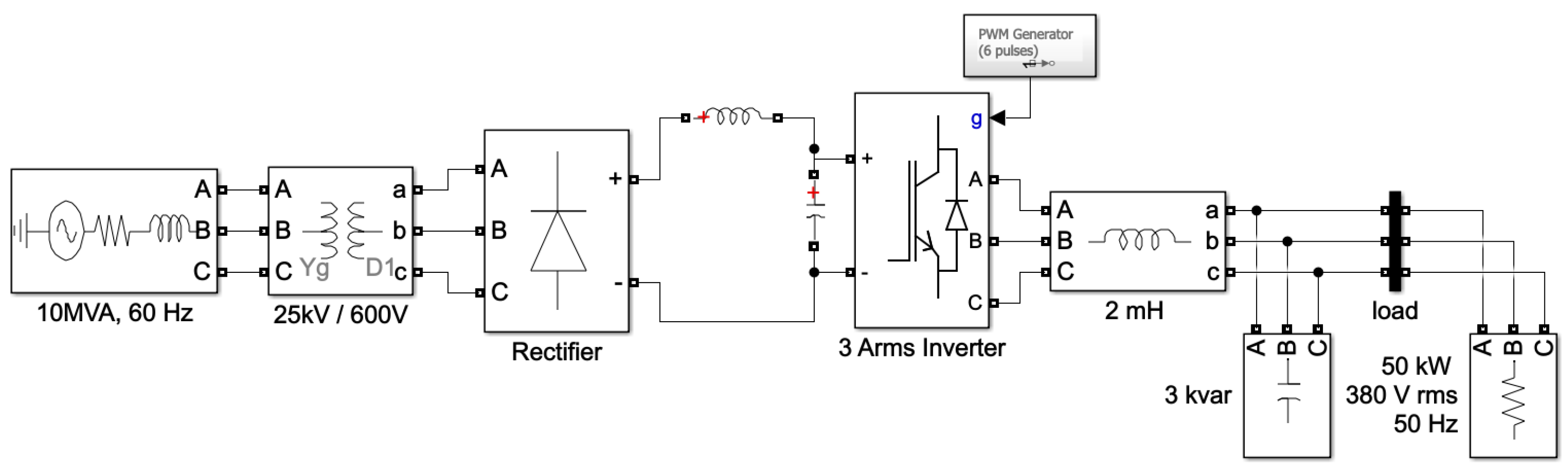
3. System Description

The $AC-DC-AC$ converter is one of several configurations explored in the literature [46,47] to decouple two frequencies. The $AC-DC-AC$ converter topology can be divided into an $AC-DC$ rectifier conversion and a $DC-AC$ inverter conversion, as shown in Figure 2. The schematic diagram of the chosen topology employs a transformer at the input, a rectifier, a DC filter, a 3-phase, 2-level inverter and an output filter before the load. The power supply is connected to the primary of the transformer. The transformer changes the primary winding voltage 25 kV into a 600 V, 60 Hz voltage obtained at the secondary of the transformer. It is then rectified by a six-pulse diode bridge. Series snubber circuits are connected in parallel with each switch device. The rectifier is expected to accomplish two main tasks: to provide a constant link voltage and to provide an almost unitary power factor. The filtered DC voltage (responsible for filtering the harmonic components at the switching frequency) is applied to an inverter generating 50 Hz. Figure 3 shows the three-phase inverter modeled with IGBT ($To{p}_i$ and $Bo{t}_i$, i = 1, 2, 3), which has two active switches with anti-parallel diodes controlled by pulse-width modulation produced by a generator. The inverter outputs are connected to a three-phase second-order filter and the filter output voltage is supplied to the load. A 60 Hz, voltage source feeds a 50 Hz 50 kW load through an $AC-DC-AC$ converter.

Table 1. Mean specifications of the $AC-DC-AC$ converter.

Especification	Parameter	Value
Input voltage	Input phase-to-phase voltage	25 kV
	Input power	10 MVA
	Grid frequency	60 Hz
Three-phase transformer Winding 1	Phase-to-phase voltage	25 kV
	Resistance	0.004 $\mathrm{\Omega }$
	Inductance	0.02 H
Three-phase transformer Winding 2	Phase-to-phase voltage	600 V
	Resistance	0.004 $\mathrm{\Omega }$
	Inductance	0.02 H
Rectifier	Snubber resistance	100 $\mathrm{\Omega }$
	Snubber capacitance	0.1 $\mathsf{\mu }$F
	Ron	0.001 $\mathrm{\Omega }$
	Foward voltage	0.8 V
Filtre DC	Inductance	200 $\mathsf{\mu }$H
	Capacitance	5 mF
Inverter	Switching frequency	50 Hz
Output filtre	Inductance	2 mH
	Capacitive reactive power	3 kVAR
Load	Phase-to-phase voltage	380 V
	Output power	50 kW
	Frequency	50 Hz

summarizes the main specifications of this $AC-DC-AC$ converter. The three-phase inverter simulation model was built using Matlab/Simulink.

One open-circuit fault may occur in the switch: $To{p}_1$ or $Bo{t}_1$ of the first phase a, $To{p}_2$ or $Bo{t}_2$ of the second phase b, $To{p}_3$ or $Bo{t}_3$ of the phase c. The case of two open-circuit faults on the upper and lower arms are $To{p}_1$ and $Bo{t}_2$, $To{p}_1$ and $Bo{t}_3$, $To{p}_2$ and $Bo{t}_1$, $To{p}_2$ and $Bo{t}_3$, $To{p}_3$ and $Bo{t}_1$, $To{p}_3$ and $Bo{t}_2$. If the upper arms are affected by the open-circuit, the two open-circuit faults can be $To{p}_1$ and $To{p}_2$, $To{p}_1$ and $To{p}_3$, $To{p}_2$ and $To{p}_3$. The two open-circuit faults, $Bo{t}_1$ and $Bo{t}_2$, $Bo{t}_1$ and $Bo{t}_3$, $Bo{t}_2$ and $Bo{t}_3$ are the symmetrical faults of the lower arms. With no loss of generality, this work is focused on the open-circuit fault on the first switch $To{p}_1$ of the first-phase a. Two open-switch faults are also considered: on the first switch $To{p}_1$ of the first-phase and on the second switch $Bo{t}_2$ of the second-phase; then, on the first switch $To{p}_1$ of the first-phase and on the first switch $To{p}_2$ of the second-phase.

4. Datasets

The growing interest in entropy approaches can be explained by their ability to analyse large sets of signals and to provide information related to their complexity. The three-phase output currents $i_a$, $i_b$ and $i_c$ collected from the inverter are measured and recorded as a one-dimensional time series to create a dataset. First, we observe the current of phase a under normal conditions when no-fault occurs in any switch of the inverter. Figure 4a shows this time-series data, sampled with sampling time T = 4 $\mathsf{\mu }$s and composed of N = 30,000 samples. In normal conditions, the currents of phases b and c are similar to those of phase a. Then, an open-circuit fault occurs in phase a on the $To{p}_1$ switch. The output currents of phases a, b and c corresponding to an open-circuit fault are shown in Figure 4a and Figure 5a,b. The $DC$ side of the output current of phase a can be observed, where two periods of $i_a$ are represented in Figure 4b. The output current of phases b and c do not change, except for a very small amplitude decrease.

Next, two open-circuit faults occur on $To{p}_1$ and $Bo{t}_2$. The corresponding output currents of phases a, b and c are shown in Figure 6a,b and Figure 7a. The open-circuit faults do not cause system shutdown but degrade the system performance. Then, two open-circuit faults occur in $To{p}_1$ and $To{p}_2$. The corresponding output currents of phases a, b and c are shown in Figure 7b and Figure 8a,b, where the $DC$ side can be observed.

The mean of the output currents of phases a, b and c, with no-fault, one open-circuit fault and two open-circuit faults occurring on the switches, is illustrated on

Table 2. Mean of the output currents of phases a, b and c with no-fault, one open-circuit fault and two open−circuit faults on the switches.

Mean	${\mathit{i}}_{\mathit{a}}$	${\mathit{i}}_{\mathit{b}}$	${\mathit{i}}_{\mathit{c}}$
No fault	−0.0034	−0.0034	−0.0034
Open circuit—$T_1$	−9.2848	4.7236	4.5612
Open circuit—$T_1$ and $B_2$	−6.8013	6.9350	−0.1337
Open circuit—$T_1$ and $T_2$	−6.2230	−6.2388	12.4618

.

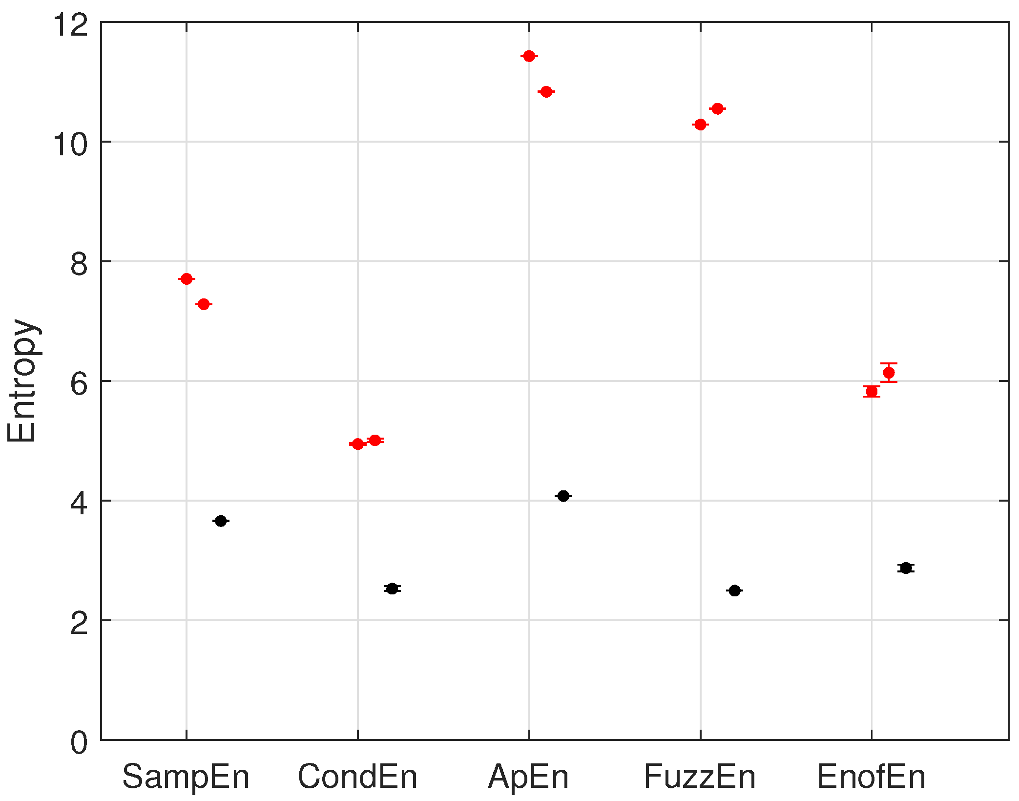
5. Results and Discussion

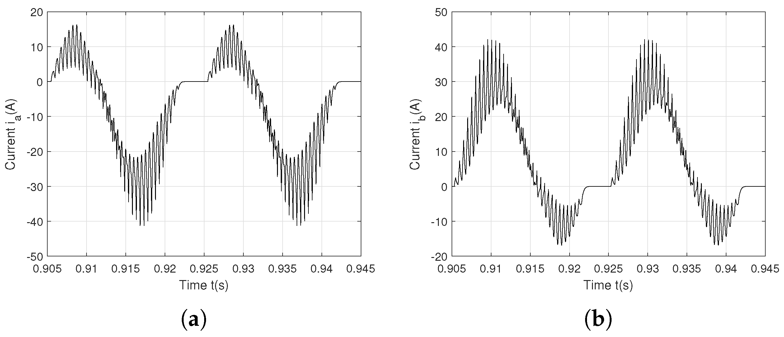
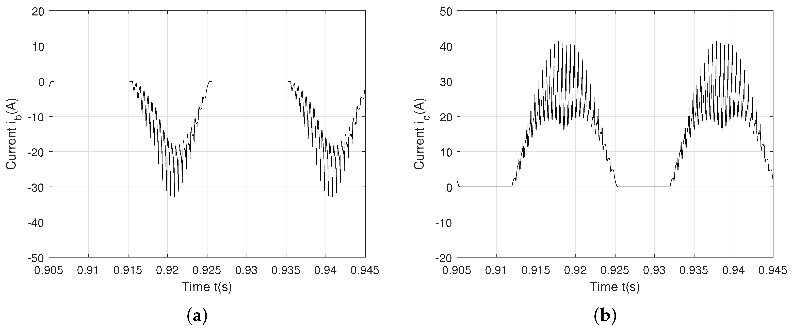
Serving as an algebraic quantification parameter, entropy is used here to characterize the complexity of different electrical signals, such as the healthy and faulty waveforms in the open-circuit case, as in Figure 4, Figure 5, Figure 6, Figure 7 and Figure 8. The block diagram of the fault detection method is presented in Figure 9. Three sensors are added to the circuit to measure the currents of the load ($i_a$, $i_b$ and $i_c$ of phases a, b and c), which can be used to identify the fault in the switch. For convenience of comparison, the entropy of phases a, b and c, when one open-circuit fault occurs on $To{p}_1$, is divided by the entropy of phase a under healthy conditions. In the same way, the entropy of phases a, b and c, when two open-circuit faults occur on $To{p}_1$ and $To{p}_2$ or $Bo{t}_2$, is divided by the entropy of phase a under healthy conditions.

All the entropies are formed as an average over two, three, or four implemented realizations. Relevant values of $MSEntropy$ and $cMSEntropy$ obtained with $SampEntropy$ were averaged to give a mean value named $SampEn$. $SampEntropy$ and $rMSEntropy$ obtained with $SampEntropy$ do not distinguish the faults occurring at different locations. Similarly, $ApEn$ represents the mean values $MSEntropy$ and $cMSEntropy$ using $ApEntropy$. Implementing the mean of $K2Entropy$, $MSEntropy$ and $cMSEntropy$ and $rMSEntropy$, used with $K2Entropy$, gives $K2En$. The mean of $CoSiEntropy$, $MSEntropy$, $cMSEntropy$ and $rMSEntropy$ (three multiscale entropies using $CoSiEntropy$) gives $CoSiEn$. $En$$\mathit{of}$$En$ was computed as the mean of the usual entropy function ($En$$\mathit{of}$$Entropy$), $MSEntropy$, $cMSEntropy$ and $rMSEntropy$, where multiscale entropy was deduced with $En$$\mathit{of}$$Entropy$. In the same way, $CondEn$ is obtained as the mean of the pertinent values of $MSEntropy$, $cMSEntropy$ and $rMSEntropy$ using $CondEntropy$. For the last mean value, $FuzzEn$ is the mean of $MSEntropy$, $cMSEntropy$ and $rMSEntropy$ using $FuzzEntropy$.

5.1. One Open-Circuit Fault on $To{p}_1$ on the Phase a

In this study, the efficiency of $SampEn$, $K2En$, $CondEn$, $CoSiEn$, $ApEn$, $FuzzEn$ and $En$$\mathit{of}$$En$ is investigated with several parameters, such as data length N = 30,000 samples, embedding dimension m = 2, time delay $\tau$ = 1, and tolerance r = 0.2 (commonly set by default). The entropy values of the 30,000 samples were calculated and are shown in Figure 10. The samples of phase a, where the open-circuit fault occurs, have larger entropy values with $SampEn$, $CondEn$, $ApEn$, $FuzzEn$ and $En$$\mathit{of}$$En$ (represented in red) than the entropy of the phase b and c (represented in black). Obviously, they are clearly separated. Even the entropy of the phase a is lower than the entropy of the phases b and c, $K2En$ and $CoSiEn$, Figure 10 also shows the separation of the three phases a, b and c: the phases b and c have an entropy very close to each other, and different to that of phase a.

Each entropy is able to detect the phase where one open-circuit fault occurs. As we can see in Figure 10, the larger difference between the entropy of phase a and the entropy of phases b and c is given by $ApEn$.

5.2. Two Open-Circuit Faults on $To{p}_1$—Phase a and on $Bo{t}_2$—Phase b

The embedding dimension m, data length N, time delay $\tau$ and the choice of tolerance r, remain unchanged. Figure 11 illustrates the performance with two open-circuit faults: on phase a with faulty $To{p}_1$ and on phase b with faulty $Bo{t}_2$. As shown below, the phases with open-circuit fault are represented in red. This time, only $SampEn$, $CondEn$, $ApEn$, $FuzzEn$ and $En$$\mathit{of}$$En$ entropies are able to detect the phase where two open-circuit faults occur. $K2En$ and $CoSiEn$ are not able to detect the two open-circuit faults on phases a and b. As we can see in Figure 11, the larger difference between the entropy of the faulty phase (a or b) and the entropy of phase c is given by $ApEn$ and $FuzzEn$.

5.3. Two Open-Circuit Faults on $To{p}_1$—Phase a and $To{p}_2$—Phase b

The parameters involved in entropy analysis were set as previously. As shown in Figure 12, the performance with two open-circuit faults can be observed on phase a with faulty $To{p}_1$ and on phase b with faulty $To{p}_2$. We investigate the phases where the two open-circuit faults occur by performing $SampEn$, $CondEn$, $FuzzEn$ and $En$$\mathit{of}$$En$. The larger difference between the entropy of the faulty phases (a and b) and the entropy of phase c is given by $FuzzEn$.

The parameters that will be discussed in the following subsections include the data length N, embedding dimension m, time lag $\tau$ and tolerance r. In order to verify the incidence of the variation parameters on the entropy, we only present the case of one open-circuit fault on $To{p}_1$.

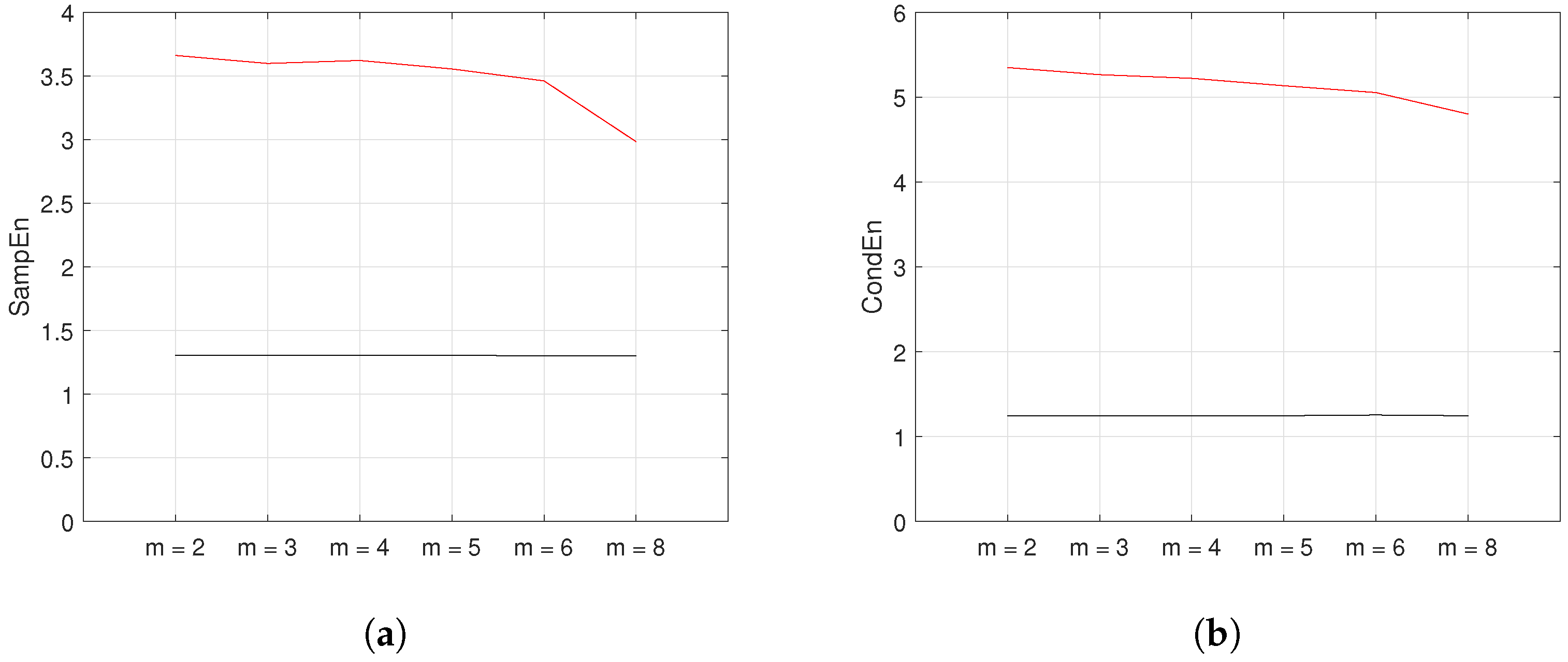
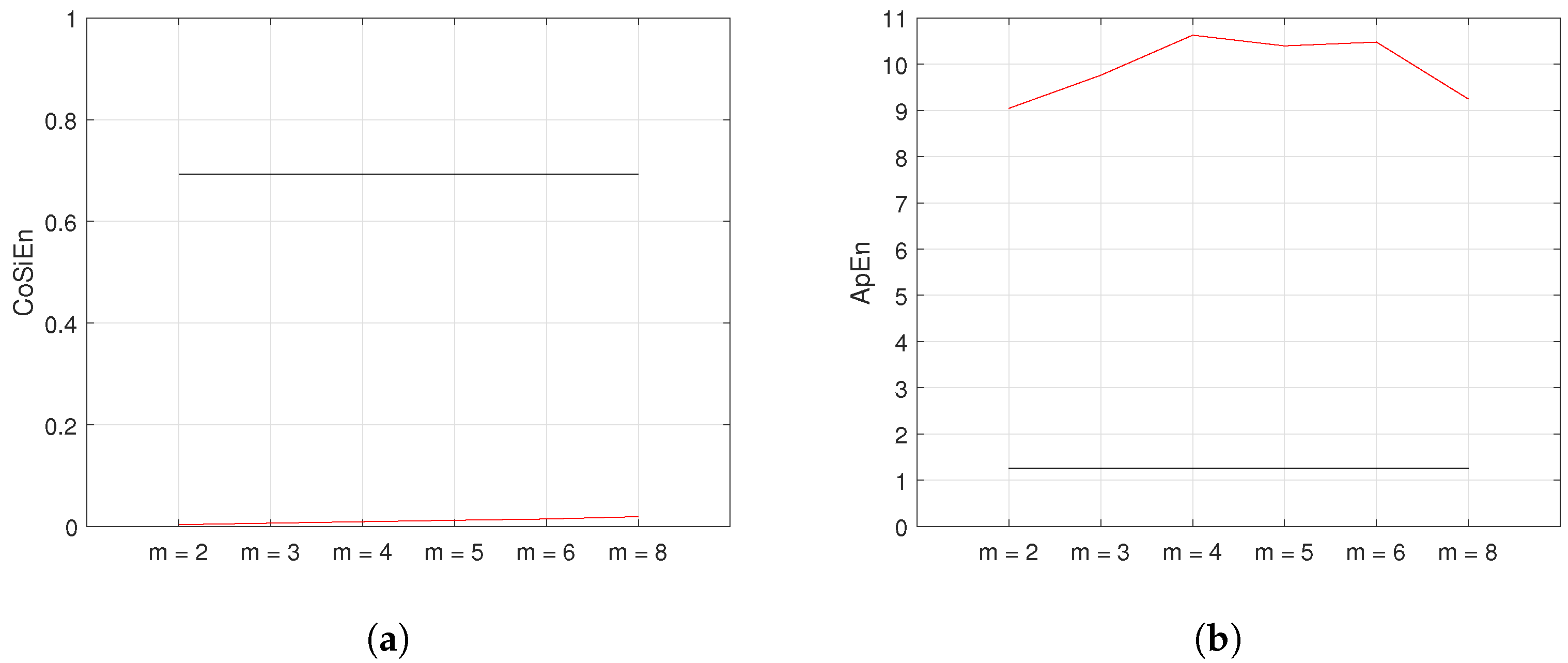
5.4. Varied Embedding Dimension (m)

Usually, for the implementation of entropy-based algorithms, the embedding dimension and data length are interdependent and mutually coupled. In practice, recorded signals have a finite length and are generally limited by processing time and memory space. Higher values of embedding dimension with a shortage of data size will cause unstable entropy estimation. Therefore, the embedding dimension is commonly set to m = 2 or m = 3 for a signal with 1000 samples. A signal with 30,000 samples approves a bigger embedding dimension with a stable entropy estimation. Here, data length, time delay and tolerance are fixed as: N = 30,000 samples, $\tau$ = 1 and r = 0.2.

Figure 13a,b show $SampEn$ and $CondEn$ as functions of the embedding dimension m. The results of $CoSiEn$ and $ApEn$ are shown in Figure 14a,b. In order to study the effect of m on these approaches ($SampEn$, $CondEn$, $CoSiEn$ and $ApEn$), we change m from 2 to 8. $SampEn$ and $CondEn$ are gradually decreased when the embedding dimension m increases. $CoSiEn$ is unchanged as m increases, keeping a constant entropy value. In Figure 14b, the relationships between $ApEn$ and the embedding dimension m show that $ApEn$ increases for m in the range (2, 4) and decreases for (6, 8). $ApEn$ is nearly constant when m is in the range (4, 6). With regards to entropy analysis and to ensure a large difference between the entropies of phases a and b, it is appropriate to choose the following values: m = 2 for $SampEn$ and $CondEn$, m = 4 for $ApEn$ and any value of m for $CoSiEn$.

5.5. Varied Data Length (N)

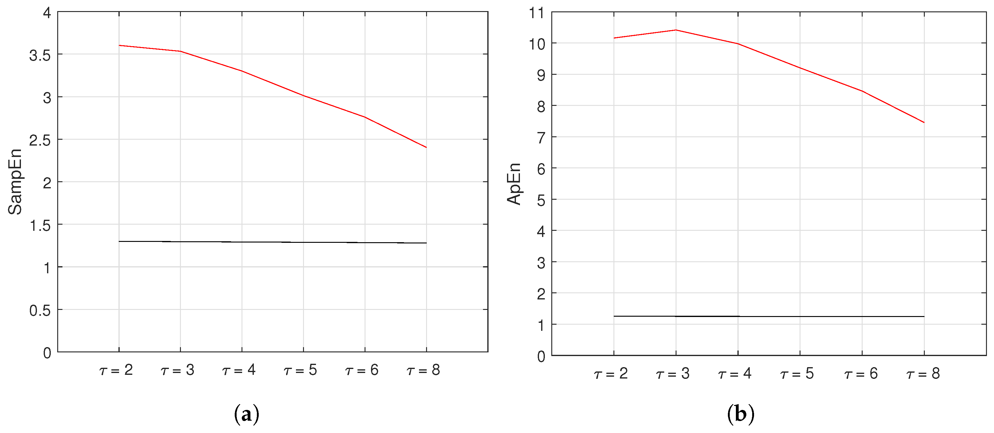
The data length of the signal is another limitation, together with the embedding dimension, when implementing the entropy calculation. The algorithms require at least 1000 data points to guarantee a consistent estimation, as for the usual entropy functions and $MSEntropy$.

Figure 15a and Figure 16b illustrate the performance of $SampEn$, $CoSiEn$, $ApEn$ and $FuzzEn$. The parameter values used to calculate the entropy are: m = 2, $\tau$ = 1 and r = 0.2. The data lengths are: $L_1$ = 6000 points, approximately two periods of the signal (Figure 4b); then the length increases up to $L_2$ = 10,000 samples; $L_3$ = 18,000 represents three periods of the signal; then 24,000 points are saved of $L_4$ data; and, finally, $L_5$ = 30,000 samples, performing six periods of the signal (Figure 4a).

The analysis of the data length, changing from 6000 samples to 30,000 samples, was only performed on $SampEn$, $CoSiEn$, $ApEn$ and $FuzzEn$. Figure 15a,b show $SampEn$ and $CoSiEn$ as functions of the data length. The results of $ApEn$ and $FuzzEn$ are shown in Figure 16a,b. $SampEn$ gradually increases with an increase in data length, as shown in Figure 15a. At the end of the scale ($L_5$ = 30,000 samples), $SampEn$ doubles compared to the initial values at $L_1$ = 6000 samples. Figure 15b shows that $CoSiEn$ remains constant when the data length increases, as in the overhead subsection. In Figure 16a, $ApEn$ increases slowly for $L_1$–$L_2$ in the sample range (6000, 10,000) and $L_3$–$L_5$ in the sample range (18,000, 30,000). $ApEn$ is nearly constant when N is in the range (10,000, 18,000). The $ApEn$ and $SampEn$ results depend on the data length. In Figure 16b, $FuzzyEn$ increases slowly for $L_1$–$L_2$ in the sample range (6000, 10,000), decreases for $L_2$–$L_3$ in the sample range (10,000, 18,000), and is followed by an increase in the range for $L_3$–$L_5$ in the sample range (18,000, 30,000). With regards to the entropy analysis, and to ensure a large difference between the entropy of phase a and the entropy of phases b and c, it is appropriate to choose a large data length for $SampEn$, $ApEn$ and $FuzzEn$. For $CoSiEn$, it is appropriate to choose $L_1$ because the entropy values are, independent of the length.

5.6. Varied Time Lag ($\tau$)

We now have a look at some representative entropies that are influenced by another indicator, such as time lag $\tau$. In this example, the time lag $\tau$ varies from 2 to 8. Having illustrated how entropy performs with data length and embedding dimension variation, we now examine the performance of $SampEn$, $ApEn$, $FuzzEn$ and $En$$\mathit{of}$$En$ with variation in time lag $\tau$. The data length, embedding dimension and tolerance were separately fixed at N = 30,000, m = 2 and r = 0.2 in the following analysis.

Figure 17a shows the impact of different $\tau$ values on $SampEn$: a monotonic decrease of $SampEn$ of phase a and a nearly constant value of phase b can be observed when $\tau$ increases. The most important difference between the two curves is for a small $\tau$. It can be observed in Figure 17b that the shape of $ApEn$ as a function of $\tau$ shows a very small increase. Then, as for $SampEn$, its values tend to decrease as $\tau$ increases. Both $ApEn$ and $SampEn$ show similar behavior for the medium and large values of time lag $\tau$. Figure 17a,b suggest that $\tau$ = 2 is suitable for the calculation of $ApEn$ and $SampEn$ values. $FuzzEn$ entropy of phases a and b with one open-circuit fault is shown in Figure 18a: only lower time-lag entropies show a relevant significance. For $\tau$ equals 1, $FuzzEn$ of the Figure 10 is 6.5, exceeding 12.5 for $\tau =2$. Furthermore, the time-lag analysis reveals additional entropy information not previously observed at time-lag 1 or 2. $FuzzEn$ clearly presents one peak for $\tau =3$: the difference between $FuzzEn$ of phase a and phase b is then maximal. However, as the time lag increases, the difference between the red and black curves becomes smaller. At the end of the $\tau$ interval, the two curves merge and the open-circuit fault on phase a cannot be detected any more. Only a lower time-lag ($\tau$ = 3) entropy has relevant significance, as in Figure 18a.

The difference between $En$$\mathit{of}$$En$ of phases a and b is nearly constant, suggesting homogeneity between them, as plotted in Figure 18a in the middle of the interval $\tau$: significant differences between $En$$\mathit{of}$$En$ of phases a and b were mostly observed at the extremities of the interval $\tau$.

5.7. Varied Tolerance (r)

The tolerance factor r varies among the experiments and is multiplied by the standard deviation entropy of phases a, b or c. In this example, the tolerance varies from 0.2 to 0.7. The data length, time lag and embedding dimension were separately fixed at N = 30,000, $\tau$ = 2 and m = 2.

Figure 19a,b present the impact of several r values on $SampEn$ and $ApEn$, respectively. Increase in r results in a monotonic increase in $SampEn$ of phase a, where the fault occurs (Figure 19a). $SampEn$ of phase b with no-fault is nearly constant, showing a very small decrease. The largest difference between the two curves is for a large r. The difference between $ApEn$ of phases a and b is nearly constant, as plotted in Figure 19b. These figures suggest that r = 0.7 is suitable for the calculation of the $ApEn$ and $SampEn$ values.

5.8. New Parameters Setting

The parameters in entropy analysis are now set to N = 30,000, m = 2, $\tau$ = 2, r = 0.7 for $SampEn$, and N = 30,000, m = 2, $\tau$ = 3, r = 0.2 for $FuzzEn$. Figure 20 shows $SampEn$ and $FuzzEn$ using $MSEn$, $cMSEn$, $rMSEn$ and the usual entropy functions $SampEntropy$ and $FuzzEntropy$, respectively, for three cases: (1) one open-circuit fault on $To{p}_1$, (2) two open-circuit faults on $To{p}_2$ and $Bo{t}_2$ and (3) two open-circuit faults on $To{p}_1$ and $To{p}_2$.

Entropy function $SampEn$: Figure 20 presents a larger difference between $SampEn$ of phases a and b than with the initial set of parameters (Figure 10) for the case (1). For cases (2) and (3), the use of the new set of parameters (Figure 20) does not lead to an improvement (cf. Figure 11 and Figure 12).

Entropy function $FuzzyEn$: for (1) the distance between $FuzzEn$ of the faulty phase a and the non-faulty phase b, considering the new setting parameters, is approximatively 12 (Figure 20), while it is near 4 with the initial set of parameters (Figure 10). Furthermore, for (2) this distance is nearly 23, as shown in Figure 20, and 8 in Figure 11, respectively. Then, for the last case (3), the distance between $FuzzEn$ of the faulty phases a and b is 26, as shown in Figure 20, and 8, respectively, with the initial set of parameters (Figure 12). Therefore, the new parameter settings enable better detection of one or several open-circuit faults, with $FuzzEn$.

6. Conclusions

Most entropy algorithms are limited to single-scale analysis, ignoring the information of other scales. Unfortunately, single-scale entropy is unable to describe the complexity of the signal and does not distinguish the faults from different phases. Multiscale analysis can fully describe the microstructural complexity and amplitude information of the signal, making it more suitable for various time-series analyses. This is why several usual entropies and multiscale entropies have been proposed to quantify the complexity of the $AC-DC-AC$ converter output currents. For some values of tolerance r and time lag $\tau$, $SampEn$ and $FuzzEn$ (using $MSEntropy$) are capable of exhibiting the complex features of the system. This paper shows the great ability of $SampEn$ and $FuzzEn$ to distinguish between a healthy state and an open-circuit faulty state. Moreover, the simulation results show that these entropies are able to detect and locate the arms of the bridge with one or even two open-circuit faults. Finally, this paper only studies single and double open-circuit faults in a three-phase inverter and checks the effectiveness of the proposed method.

In the future, we will increase the number of multilevel converter levels and introduce more fault types for comprehensive fault diagnosis. Moreover, it will be possible to study the diagnosis method of the inverter, where the open-circuit fault occurs, and to add a fault-tolerant strategy to ensure that the inverter can work normally.

References

1. Hu, P.; Jiang, D.; Zhou, Y.; Liang, Y.; Guo, J.; Lin, Z. Energy-balancing control strategy for modular multilevel converters under SM fault conditions. IEEE Trans. Power Electron. 2014, 29, 5021–5030. [Google Scholar] [CrossRef]
2. Yang, S.; Tang, Y.; Wang, P. Open-circuit fault diagnosis of switching devices in a modular multilevel converter with distributed control. In Proceedings of the IEEE Energy Conversion Congress and Exposition (ECCE), Cincinnati, OH, USA, 1–5 November 2017; pp. 4208–4214. [Google Scholar]
3. Perez, M.A.; Bernet, S.; Rodriguez, J.; Kouro, S.; Lizana, R. Circuit topologies, modeling, control schemes, and applications of modular multilevel converters. IEEE Trans. Power Electon. 2015, 30, 4–17. [Google Scholar] [CrossRef]
4. Rong, F.; Gong, X.; Huang, S. A Novel Grid-Connected PV System Based on MMC to Get the Maximum Power Under Partial Shading Conditions. IEEE Trans. Power Electron. 2015, 32, 4320–4333. [Google Scholar] [CrossRef]
5. Estima, J.; Cordoso, A.J.M. A new approach for real-time multiple open-circuit fault diagnosis in volt-age-source inverters. IEEE Trans. Ind. Appl. 2011, 47, 2487–2494. [Google Scholar] [CrossRef]
6. Li, B.; Zhou, S.; Xu, D.; Yang, R.; Xu, D.; Buccella, C.; Cecati, C. An improved circulating current injection method for modular multilevel converters in variable-speed drives. IEEE Trans. Ind. Electron. 2016, 63, 7215–7225. [Google Scholar] [CrossRef]
7. Huo, Z.; Miguel Martínez-García, M.; Zhang, Y.; Yan, R.; Shu, L. Entropy Measures in Machine Fault Diagnosis: Insights and Applications. IEEE Trans. Instrum. Meas. 2020, 69, 2607–2620. [Google Scholar] [CrossRef]
8. Ahmadi, S.; Poure, P.; Saadate, S.; Khaburi, D.A. A Real-Time Fault Diagnosis for Neutral-Point-Clamped Inverters Based on Failure-Mode Algorithm. IEEE Trans. Ind. Inform. 2021, 17, 1100–1110. [Google Scholar] [CrossRef]
9. Caseiro, L.M.A.; Mendes, A.M.S. Real-time IGBT open-circuit fault diagnosis in three-level neutral-point-clamped voltage-source rectifiers based on instant voltage error. IEEE Trans. Ind. Electron. 2015, 62, 1669–1678. [Google Scholar] [CrossRef]
10. Nsaif, Y.; Lipu, M.S.H.; Hussain, A.; Ayob, A.; Yusof, Y.; Zainuri, M.A. A New Voltage Based Fault Detection Technique for Distribution Network Connected to Photovoltaic Sources Using Variational Mode Decomposition Integrated Ensemble Bagged Trees Approach. Energies 2022, 15, 7762. [Google Scholar] [CrossRef]
11. Lee, J.S.; Lee, K.B.; Blaabjerg, F. Open-switch fault detection method of a back-to-back converter using NPC topology for wind turbine systems. IEEE Trans. Ind. Appl. 2014, 51, 325–335. [Google Scholar] [CrossRef]
12. Yu, L.; Zhang, Y.; Huang, W.; Teffah, K. A fast-acting diagnostic algorithm of insulated gate bipolar transistor open circuit faults for power inverters in electric vehicles. Energies 2017, 10, 552. [Google Scholar] [CrossRef] [Green Version]
13. Park, B.G.; Lee, K.J.; Kim, R.Y.; Kim, T.S.; Ryu, J.S.; Hyun, D.S. Simple fault diagnosis based on operating characteristic of brushless direct-current motor drives. IEEE Trans. Ind. Electron. 2011, 58, 1586–1593. [Google Scholar] [CrossRef]
14. Faraz, G.; Majid, A.; Khan, B.; Saleem, J.; Rehman, N. An Integral Sliding Mode Observer Based Fault Diagnosis Approach for Modular Multilevel Converter. In Proceedings of the 2019 International Conference on Electrical, Communication, and Computer Engineering (ICECCE), Swat, Pakistan, 24–25 July 2019; pp. 1–6. [Google Scholar]
15. Song, B.; Qi, G.; Xu, L. A new approach to open-circuit fault diagnosis of MMC sub-module. Syst. Sci. Control Eng. 2020, 8, 119–127. [Google Scholar] [CrossRef] [Green Version]
16. Deng, F.; Chen, Z.; Khan, M.; Zhu, R. Fault Detection and Localization Method for Modular Multilevel Converters. IEEE Trans. Power Electron. 2015, 30, 2721–2732. [Google Scholar] [CrossRef]
17. Zhang, Y.; Hu, H.; Liu, Z. Concurrent fault diagnosis of a modular multi-level converter with kalman filter and optimized support vector machine. Syst. Sci. Control Eng. 2019, 7, 43–53. [Google Scholar] [CrossRef] [Green Version]
18. Volonescu, C. Fault Detection and Diagnosis; IntechOpen: London, UK, 2018; ISBN 13 978-1789844368. [Google Scholar]
19. Estima, J.O.; Freire, N.M.A.; Cardoso, A.J.M. Recent advances in fault diagnosis by Park’s vector approach. IEEE Workshop Electr. Mach. Des. Control Diagn. 2013, 2, 279–288. [Google Scholar]
20. Wang, C.; Lizana, F.; Li, Z. Submodule short-circuit fault diagnosis based on wavelet transform and support vector machines for a modular multi-level converter with series and parallel connectivity. In Proceedings of the IECON 2017—43rd Annual Conference of the IEEE Industrial Electronics Society, Beijing, China, 29 October–1 November 2017; pp. 3239–3244. [Google Scholar]
21. Xing, W. An open-circuit fault detection and location strategy for MMC with feature extraction and random forest. In Proceedings of the 2021 IEEE Applied Power Electronics Conference and Exposition (APEC), Phoenix, AZ, USA, 14–17 June 2021; pp. 1111–1116. [Google Scholar]
22. Wang, Q.; Yu, Y.; Hoa, A. Fault detection and classification in MMC-HVDC systems using learning methods. Sensors 2020, 20, 4438. [Google Scholar] [CrossRef]
23. Morel, C.; Akrad, A.; Sehab, R.; Azib, T.; Larouci, C. IGBT Open-Circuit Fault-Tolerant Strategy for Interleaved Boost Converters via Filippov Method. Energies 2022, 15, 352. [Google Scholar] [CrossRef]
24. Li, T.; Zhao, C.; Li, L.; Zhang, F.; Zhai, X. Sub-module fault diagnosis and local protection scheme for MMC-HVDC system. Proc. CSEE 2014, 34, 1641–1649. [Google Scholar]
25. Mendes, A.; Cardoso, A.; Saraiva, E.S. Voltage source inverter fault diagnosis in variable speed AC drives, by the average current Park’s vector approach. In Proceedings of the IEEE International Electric Machines and Drives Conference, Seattle, WA, USA, 9–12 May 1999; pp. 704–706. [Google Scholar]
26. Ke, L.; Liu, Z.; Zhang, Y. Fault Diagnosis of Modular Multilevel Converter Based on Optimized Support Vector Machine. In Proceedings of the 2020 39th Chinese Control Conference, Shenyang, China, 27–29 July 2020; pp. 4204–4209. [Google Scholar]
27. Geng, Z.; Wang, Q.; Han, Y.; Chen, K.; Xie, F.; Wang, Y. Fault Diagnosis of Modular Multilevel Converter Based on RNN and Wavelet Analysis. In Proceedings of the 2020 Chinese Automation Congress, Shanghai, China, 6–8 November 2020; pp. 1097–1101. [Google Scholar]
28. Wang, S.; Bi, T.; Jia, K. Wavelet entropy based single pole grounding fault detection approach for MMC-HVDC overhead lines. Power Syst. Technol. 2016, 40, 2179–2185. [Google Scholar]
29. Shen, Y.; Wang, T.; Amirat, Y.; Chen, G. IGBT Open-Circuit Fault Diagnosis for MMC Submodules Based on Weighted-Amplitude Permutation Entropy and DS Evidence Fusion Theory. Machines 2021, 9, 317. [Google Scholar] [CrossRef]
30. Richman, J.; Randall Moorman, J. Physiological time-series analysis using approximate entropy and sample entropy. Am. J. Physiol. Heart Circ. Physiol. 2000, 278, 2039–2049. [Google Scholar] [CrossRef] [Green Version]
31. Unakafova, V.; Unakafov, A.; Keller, K. An approach to comparing Kolmogorov-Sinai and permutation entropy. Eur. Phys. J. 2013, 222, 353–361. [Google Scholar] [CrossRef] [Green Version]
32. Porta, A.; Baselli, G.; Liberati, D.; Montano, N.; Cogliati, C.; Gnecchi-Ruscone, T.; Malliani, A.; Cerutti, S. Measuring regularity by means of a corrected conditional entropy in sympathetic outflow. Biol. Cybern. 1998, 78, 71–78. [Google Scholar] [CrossRef] [PubMed]
33. Theerasak, C.; Mandic, D. Cosine Similarity Entropy: Self-Correlation-Based Complexity Analysis of Dynamical Systems. Entropy 2017, 19, 652. [Google Scholar]
34. Azami, H.; Li, P.; Arnold, S.; Escuder, J.; Humeau-Heurtier, A. Fuzzy Entropy Metrics for the Analysis of Biomedical Signals: Assessment and Comparison. IEEE Access 2016, 4, 1–16. [Google Scholar] [CrossRef]
35. Chen, W.; Wang, Z.; Xie, H.; Yu, W. Characterization of surface EMG signal based on fuzzy entropy, Neural Systems and Rehabilitation Engineering. IEEE Trans. Neural Syst. Rehabil. Eng. 2007, 15, 266–272. [Google Scholar] [CrossRef] [PubMed]
36. Chang, F.; Sung-Yang, W.; Huang, H.P.; Hsu, L.; Chi, S.; Peng, C.K. Entropy of Entropy: Measurement of Dynamical Complexity for Biological Systems. Entropy 2017, 19, 550. [Google Scholar]
37. Costa, M.; Goldberger, A.; Peng, C. Multiscale entropy analysis of complex physiologic time series. Phys. Rev. Lett. 2002, 89, 068102. [Google Scholar] [CrossRef] [Green Version]
38. Costa, M.; Goldberger, A.; Peng, C. Multiscale entropy analysis of biological signals. Phys. Rev. E 2005, 71, 021906. [Google Scholar] [CrossRef] [Green Version]
39. Liu, T.; Cui, L.; Zhang, J.; Zhang, C. Research on fault diagnosis of planetary gearbox based on Variable Multi-Scale Morphological Filtering and improved Symbol Dynamic Entropy. Int. J. Adv. Manuf. Technol. 2023, 124, 3947–3961. [Google Scholar] [CrossRef]
40. Silva, L.; Duque, J.; Felipe, J.; Murta, L.; Humeau-Heurtier, A. Twodimensional multiscale entropy analysis: Applications to image texture evaluation. Signal Process. 2018, 147, 224–232. [Google Scholar] [CrossRef]
41. Morel, C.; Humeau-Heurtier, A. Multiscale permutation entropy for two-dimensional patterns. Pattern Recognit. Lett. 2021, 150, 139–146. [Google Scholar] [CrossRef]
42. Valencia, J.; Porta, A.; Vallverdu, M.; Claria, F.; Baranovski, R.; Orlowska-Baranovska, E.; Caminal, P. Refined multiscale entropy: Application to 24-h Holter records of heart period variability in hearthy and aortic stenosis subjects. IEEE Trans. Biomed. Eng. 2009, 56, 2202–2213. [Google Scholar] [CrossRef] [PubMed]
43. Wu, S.; Wu, C.; Lin, S.; Lee, K.; Peng, C. Analysis of complex time series using refined composite multiscale entropy. Phys. Lett. A 2014, 378, 1369–1374. [Google Scholar] [CrossRef]
44. Wu, S.; Wu, C.; Lin, S.; Wang, C.; Lee, K. Time series analysis using composite multiscale entropy. Entropy 2013, 15, 1069–1084. [Google Scholar] [CrossRef] [Green Version]
45. Humeau-Heurtier, A. The Multiscale Entropy Algorithm and Its Variants: A Review. Entropy 2015, 17, 3110–3123. [Google Scholar] [CrossRef] [Green Version]
46. Dai, M.; Marwali, M.N.; Jung, J.-W.; Keyhani, A. A Three-Phase Four-Wire Inverter Control Technique for a Single Distributed Generation Unit in Island Mode. IEEE Trans. Power Electron. 2008, 23, 322–331. [Google Scholar] [CrossRef]
47. Raja, N.; Mathewb, J.; Ga, J.; George, S. Open-Transistor Fault Detection and Diagnosis Based on Current Trajectory in a Two-level Voltage Source Inverter. Procedia Technol. 2016, 25, 669–675. [Google Scholar] [CrossRef] [Green Version]
Figure 1. MSEntropy.
Energies 16 01959 g001
Figure 2. Power circuit structure of a  A C D C A C  converter.
Energies 16 01959 g002
Figure 3. Schematic representation of a three-phase, two-level inverter.
Energies 16 01959 g003
Figure 4. The output current of phase a: (a) Current  i a  under no-fault case; (b) Current  i a  when open-circuit fault on  T o p 1 .
Energies 16 01959 g004
Figure 5. The output currents: (a) Current  i b  when open-circuit fault on  T o p 1 ; (b) Current  i c  when open-circuit fault on  T o p 1 .
Energies 16 01959 g005
Figure 6. The output currents: (a) Current  i a  when open-circuit faults on  T o p 1  and  B o t 2 ; (b) Current  i b  when open-circuit faults on  T o p 1  and  B o t 2 .
Energies 16 01959 g006
Figure 7. The output currents: (a) Current  i c  when open-circuit faults on  T o p 1  and  B o t 2 ; (b) Current  i a  when open-circuit faults on  T o p 1  and  T o p 2 .
Energies 16 01959 g007
Figure 8. The output currents: (a) Current  i b  when open-circuit faults on  T o p 1  and  T o p 2 ; (b) Current  i c  when open-circuit faults on  T o p 1  and  T o p 2 .
Energies 16 01959 g008
Figure 9. Block diagram representation of the faults detection method.
Energies 16 01959 g009
Figure 10. Entropy evaluation using  M S E n c M S E n r M S E n  and the usual entropy functions for one open-circuit fault on  T o p 1 : entropy of phase a with open-circuit fault represented in red and entropy of phases b and c in black.
Energies 16 01959 g010
Figure 11. Entropy evaluation using  M S E n c M S E n r M S E n  and the usual entropy functions for two open-circuit faults on  T o p 1  and on  B o t 2 : entropy of the phases a and b with open-circuit fault represented in red and the entropy of phase c in black.
Energies 16 01959 g011
Figure 12. Entropy evaluation using  M S E n c M S E n r M S E n  and the usual entropy functions for two open-circuit faults on  T o p 1  and on  T o p 2 : entropy of phases a and b with open-circuit fault represented in red and entropy of phase c in black.
Energies 16 01959 g012
Figure 13. (a) Mean of  M S E n  and  c M S E n  computed with  S a m p E n t r o p y  and (b) mean of  M S E n c M S E n  and  r M S E n  computed with  C o n d E n t r o p y  for the embedding dimension m: entropy of phase a with open-circuit fault represented in red and entropy of phase b in black.
Energies 16 01959 g013
Figure 14. (a) Mean of  M S E n c M S E n  and  r M S E n  computed with  C o S i E n t r o p y  and (b) mean of  M S E n  and  c M S E n  computed with  A p E n t r o p y  for the embedding dimension m: entropy of phase a with open-circuit fault represented in red and entropy of phase b in black.
Energies 16 01959 g014
Figure 15. (a) Mean of  M S E n  and  c M S E n  computed with  S a m p E n t r o p y  and (b) mean of  M S E n c M S E n  and  r M S E n  computed with  C o S i E n t r o p y  for the data length N: entropy of phase a with open-circuit fault represented in red and entropy of phases b and c in black.
Energies 16 01959 g015
Figure 16. (a) Mean of  M S E n  and  c M S E n  computed with  A p E n t r o p y  and (b) mean of  M S E n c M S E n  and  r M S E n  computed with  F u z z E n t r o p y  for the data length N: entropy of phase a with open-circuit fault represented in red and entropy of phases b and c in black.
Energies 16 01959 g016
Figure 17. (a) Mean of  M S E n  and  c M S E n  computed with  S a m p E n t r o p y  and (b) mean of  M S E n  and  c M S E n  computed with  A p E n t r o p y  for the time lag  τ : entropy of phase a with open-circuit fault represented in red and entropy of phase b in black.
Energies 16 01959 g017
Figure 18. (a) Mean of  M S E n c M S E n  and  r M S E n  computed with  F u z z E n t r o p y  and (b) mean of  M S E n c M S E n  and  r M S E n  computed with  E n of E n t r o p y  for the time lag  τ : entropy of phase a with open-circuit fault represented in red and entropy of phase b in black.
Energies 16 01959 g018
Figure 19. (a) Mean of  M S E n  and  c M S E n  computed with  S a m p E n t r o p y  and (b) mean of  M S E n  and  c M S E n  computed with  A p E n t r o p y  for the tolerance r: entropy of phase a with open-circuit fault represented in red and entropy of phase b in black.
Energies 16 01959 g019
Figure 20. Entropy evaluation using  M S E n c M S E n r M S E n  and usual entropy functions: for open-circuit fault on  T o p 1  (phase a in red, phases b and c in black), for two open-circuit faults on  T o p 1  (phase a in red) and  B o t 2  (phase b in red) phase c in black, and two open-circuit faults on  T o p 1  (phase a in red) and  T o p 2  (phase b in red) phase c in black.
Energies 16 01959 g020