Prestack Seismic Velocity Ratio Evaluation of a Mixed Siliciclastic–Carbonate Formation: Case Study from the Strawn Group on the Eastern Shelf Texas

Abstract

Although a mixed carbonate–siliciclastic system of the Strawn Group on the Eastern Shelf in King County, Texas, USA provides excellent hydrocarbon reservoirs, facies variability and reservoir properties within such systems are not well understood. We conducted prestack, simultaneous seismic inversion, and high-level petrophysical analysis to derive elastic properties of rocks to facilitate lithology identification and determination and distribution of the different carbonate facies. Our results show that (1) the Strawn Group in King County is dominated mostly by carbonates and (2) given the ratio of P- and S-wave velocity (Vp/Vs ratio), the carbonates can be separated into three facies: (a) high-Vp/Vs-ratio shelf-edge reef carbonates, in which the Vp/Vs ratio decreases linearly as porosity increases and the Vp/Vs ratio varies from ~2.1 to ≤2.6; (b) moderately low-Vp/Vs-ratio shelf (platform) carbonates, in which the Vp/Vs ratio also decreases as porosity increases and in which the Vp/Vs ratio ranges from ~1.75 to ≤2.15; (c) extremely low-Vp/Vs-ratio slope and basin carbonates, in which the Vp/Vs ratio, although appearing to be almost constant for a wide range of porosity, increases as porosity increases, and in which most Vp/Vs-ratio values appear to range from ~1.5 to ≤2. Results of a through c can be summarized thusly: the Vp/Vs ratio of reef carbonates >the Vp/Vs ratio of platform carbonates and >the Vp/Vs ratio of slope and basin carbonates in the study area.

1. Introduction

Although mixed carbonate—siliciclastic systems, including the Central Basin Platform and Eastern Shelf of the Permian Basin, are known around the world, facies variability and reservoir properties within such systems are not well understood [1,2]. Such heterolithic systems are formed either from the mixing of carbonate and siliciclastic detritus from the shelf (spatially mixed) or the formation of alternating successions of carbonates and siliciclasts from allocyclic or autocyclic processes (temporally mixed) [2,3]. Additionally, evaporitic reflux, subaerial exposure, and later burial-driven processes drive a complex diagenetic paragenesis that blurs the depositional generated flow-unit structure, as well as making mineralogic mapping challenging. The carbonate—silica (+/−clay, depending on a humid vs. an arid system) ratio plays a key role in reservoir properties and the heterolithic nature of the mixed siliciclastic/carbonate successions affects seismic and rock-physics responses, making reservoir characterization more challenging. We investigated the seismic response of the Strawn Group on the Eastern Shelf in King County, North Central Texas, covering an area of ~162 mi² (420 km²) (Figure 1), the Pennsylvanian (Desmoinesian) Strawn Group consisting of terrigenous clastic and carbonate facies that had been deposited within the Fort Worth Basin and on the adjacent Concho Platform (Eastern Shelf) of North Central Texas [4,5]. Researchers have long recognized 12 cycles involving a smooth interchange of deltaic progradation (sea-level fall, regressive) and marine transgression (sea-level rise) [4].

During transgression, carbonate facies accumulate as thick offshore bank systems and migrate landward as transgressive limestone [4]. In both cases (transgression and progradation), deposition and erosion of previously deposited sediments are involved. The shelf landscape is thus modified, featuring hills (topographic highs) and valleys (gullies). Some workers have noted that within the Strawn Group in King County, both carbonates and clastics provide excellent hydrocarbon reservoirs from depths of ~5000 to 6000 ft (1524 to 1830 m) [6]. From early 1940 to ~1993, >100 million barrels (MMbbl) of oil was produced from the Strawn [6] and the presence of commercial hydrocarbon within the Strawn Group has provided the incentives for continued exploration of these formations in King and adjacent counties.

On the basis of work by several researchers, e.g., [7,8], continued exploration and exploitation of the Strawn Group for hydrocarbon has been facilitated by the extraction of elastic properties of the rocks via prestack, simultaneous inversion for the purposes of lithologic identification, and proper reservoir characterization. Through the extraction of elastic properties, such as density [9,10] and acoustic impedance [7], siliciclastics have been distinguished from carbonates and lithology-composing topographic highs in a mixed lithologic landscape have been inferred. The ratio of P- to S-wave velocity (Vp/Vs ratio) is another useful elastic property of the rock that can be derived from seismic and petrophysical data. In seismic data interpretation, the Vp/Vs ratio plays a key role in the determination of character and lithological composition of rocks [11,12]. Several case studies have demonstrated the usefulness of the Vp/Vs ratio in differentiating lithological facies. For example, some workers used the Vp/Vs ratio to distinguish a sandstone-rich zone from a shale-rich zone in the Empire Abo field, New Mexico [6]. They showed that the sandstone-rich zone has a lower Vp/Vs ratio than the shale-rich zone. By plotting the Vp/Vs ratio and the neutron-log-derived porosity along a seismic traverse in the Kingfisher field, Oklahoma, researchers showed that the porosity increased from west to east as the Hunton carbonate rock changed from limestone to dolomite and the porosity continued to increase with increasing dolomitization [13]. This change in porosity correlated with where the Vp/Vs ratio started to increase eastward, suggesting that the Vp/Vs ratio increases with increasing porosity and implying that porous zones within carbonate rocks can be identified using the Vp/Vs ratio. Other researchers, working in the Scipio field, Michigan, identified a porous zone (dolomitized zone) within the Trenton to Prairie du Chien interval by plotting the Vp/Vs ratio along a seismic profile line [14]. These authors showed that the dolomitized (porous) zone could be identified by a drop in the Vp/Vs ratio, from ~1.9 for limestone to 1.8 or lower for dolomite; although, here, the Vp/Vs ratio decreases as porosity increases, note that the Vp/Vs ratio generally depends on many factors such as porosity, degree of consolidation, clay content, differential pressure, type of fluid in pore spaces, pore geometry, aspect ratios of cracks, rate of fluid saturation, and other factors [15,16]. Other workers showed that the Vp/Vs ratio increases linearly with increasing shaliness [17]; still others showed that the Vp/Vs ratio of dry rock or gas-saturated rock remains almost constant, irrespective of porosity or differential pressure, whereas the Vp/Vs ratio of wet rock is porosity- and differential pressure-dependent [18]. Finally, some authors showed that, with increasing porosity, the Vp/Vs ratio decreases if porosity is saturated with water, whereas it increases if porosity is saturated with a much less compressible fluid such as melt [19].

Given the depositional history of the Strawn Group, the objectives of our investigation were to (1) identify the remnant topographic highs (anticlinal structures) that normally serve as potential hydrocarbon reservoirs and (2) determine the distribution of elastic parameters, namely the Vp/Vs ratio and density and impedance of the rocks and, hence, infer the nature and lithologic composition of the Strawn Group in the study area. Although there are other methods that could be employed to address these tasks, such as image segmentation [20] and artificial intelligence, e.g., [21], we used the prestack simultaneous seismic inversion method, which is more applicable to the problem at hand.

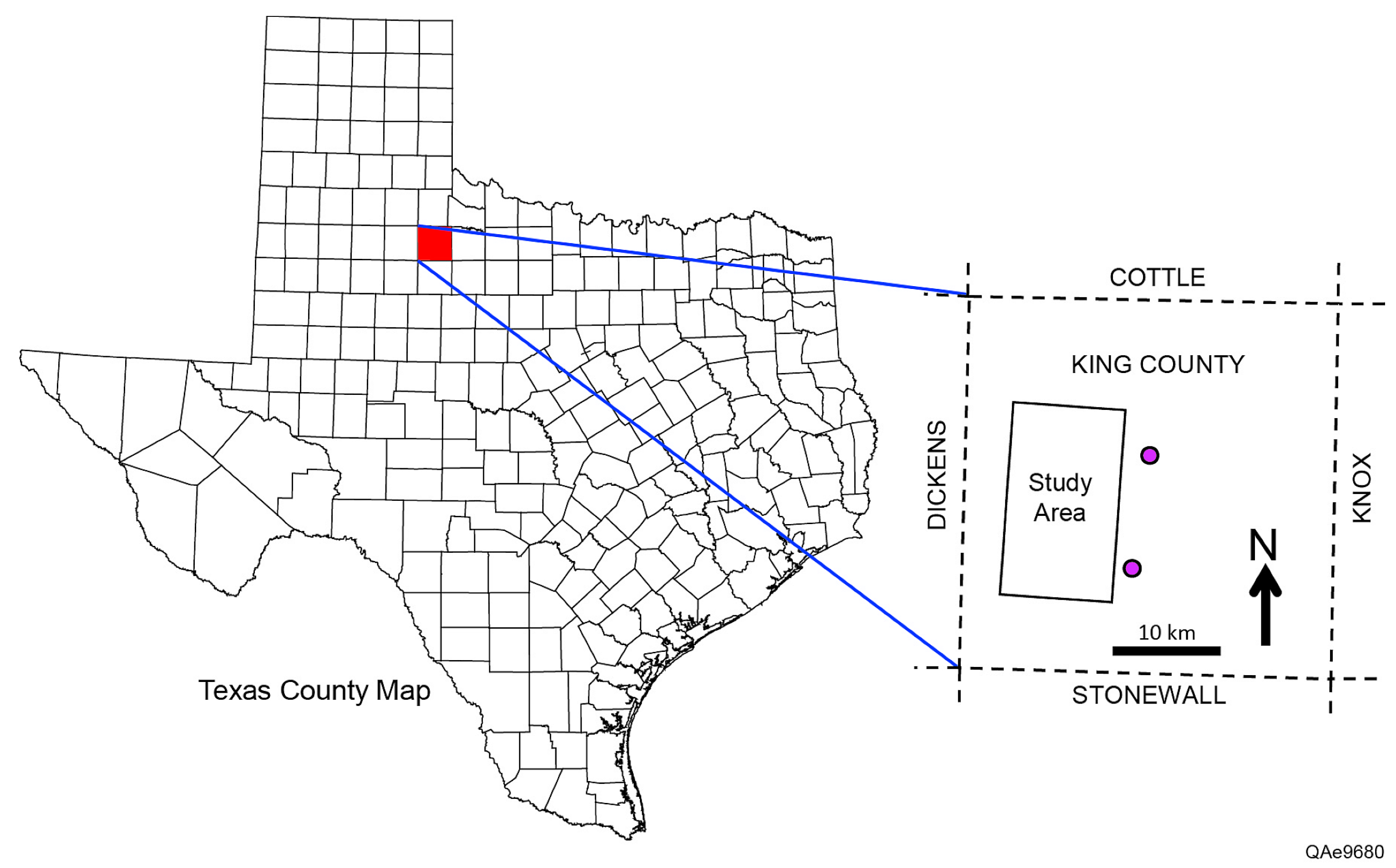
2. Geology

The Strawn Group is part of the sedimentary rock succession that was deposited on top of the Concho Platform between the early Desmoinesian and the end of the Missourian (Figure 2). The Concho Platform is a lower and middle Paleozoic positive structural element in North Central Texas that was later modified by subsidence in the adjoining Fort Worth foreland basin to the east and northeast and the Midland Basin to the west [4,5]. The platform is bound to the north by the Matador Arch, the Red River Uplift, and the Muenster Arch, which together represent a discontinuous east–west-trending series of aligned block-faulted structural highs [4,5].

Sedimentation of the Strawn Group on top of the Concho Platform began when epeirogenic uplift of the Fort Worth Basin caused a gradual tilting of the entire Concho Platform westward during the late Desmoinesian [4,5,22]. The tilting of the platform led to a reversal of sedimentation direction from east to west, thus beginning deposition of the Strawn Group on top of the Concho Platform and across the Eastern Shelf and into the Midland Basin. During progradation, depocenters can switch from place to place because of a low slope gradient [23] and the shelf, as well as the shoreline, can be eroded. These eroded materials, together with the sediments from the hinterland (provenance areas), are then deposited on the shelf, forming constructional lobate and elongate delta systems [4,5,6]. Through erosional cutout valleys, some of these transported sediments are funneled downslope across the shelf edge into the basin [6]. The Strawn Group is generally composed of sandstone, siltstone, and shale, with thin discontinuous carbonates and coal. However, to the west, in the Eastern Shelf area of the Midland Basin and King County, it is composed of alluvial to open-shelf clastics (shales and siltstones) and platform-to-ramp carbonates, basinal carbonates, and marine shales [24,25].

3. Database

The well database consists of eight wells that have been drilled into the Strawn Group. The log suites are spontaneous potential (SP), gamma-ray, resistivity, density, P-wave sonic (Vp), S-wave sonic (Vs), and interpreted lithology logs, as well as checkshot data. Our 3D seismic database comprises prestack normal and moveout-corrected (NMO) angle-gathers, sampled at 2 ms, and having a stacking bin size of 17 × 17 m. We also had a stacked migrated seismic volume that we used to interpret four key horizons. The lines of cross sections A–A’, B–B’, C–C’, and D–D’ (Figure 3) can explain the nature of some of the carbonates observed in the area of investigation.

4. Methods

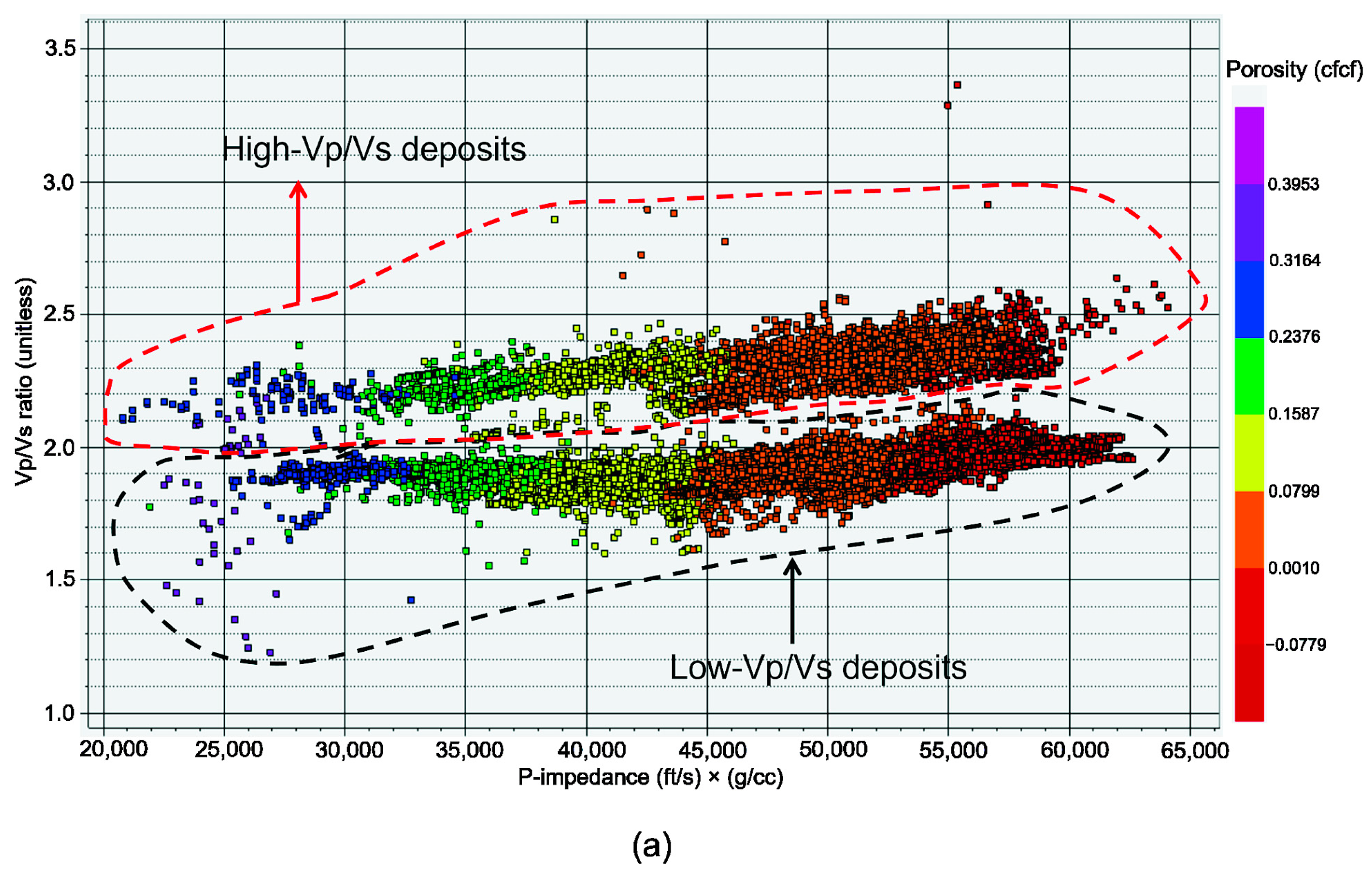
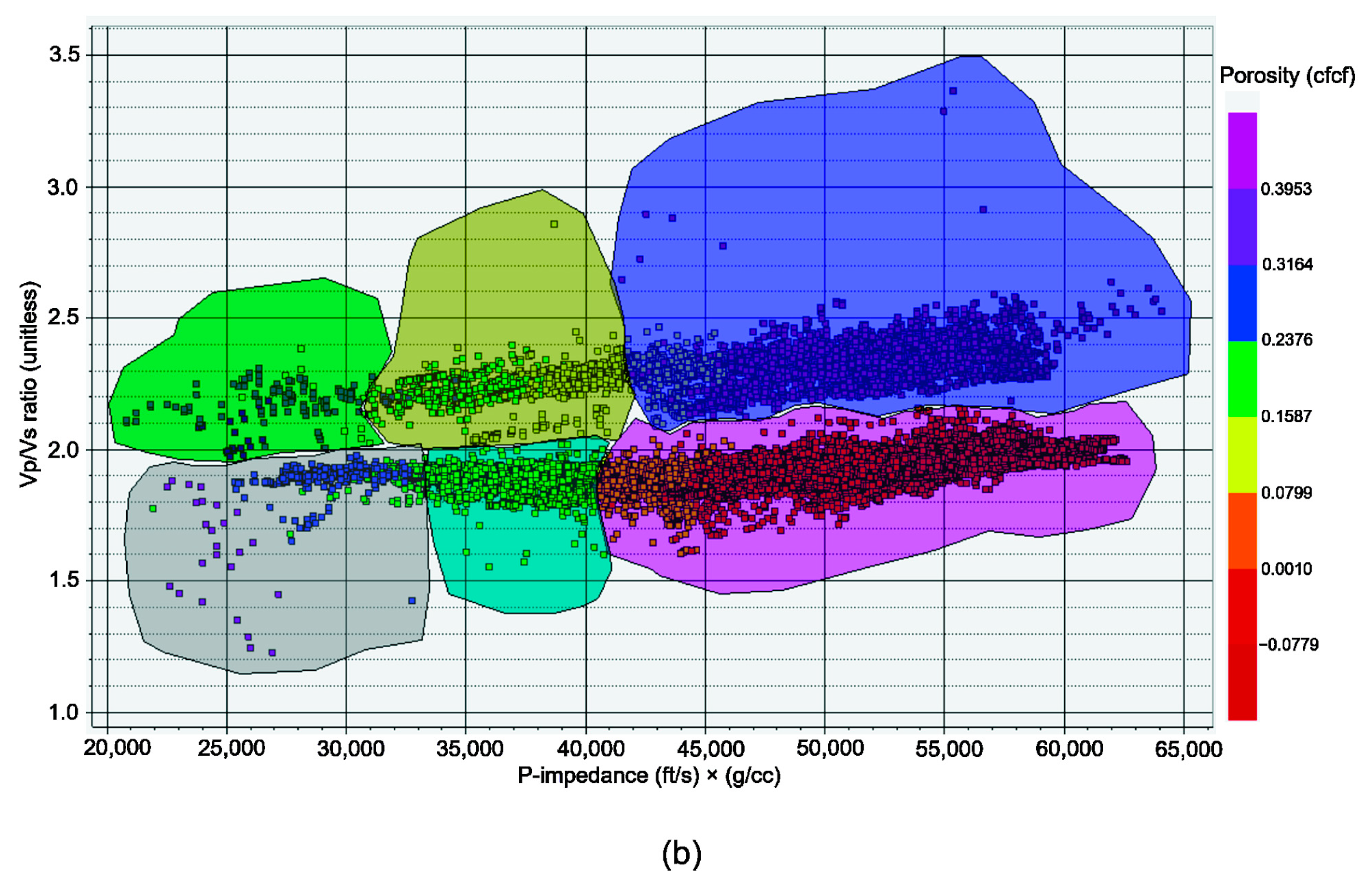
4.1. Cross Plots of Velocity Ratio (Vp/Vs) Versus Impedance

To determine the different types of lithology within the Strawn Group, we generated cross plots of the ratio of P-wave to S-wave velocity (Vp/Vs ratio) versus P-impedance, color-coded with porosity, using the eight wells. A plot (Figure 4) shows that (1) given the Vp/Vs ratio, two separate linear trends occur, suggesting that the Strawn Group is composed of two types of sedimentary deposits ((a) low-Vp/Vs-ratio deposits and (b) high-Vp/Vs-ratio deposits) and (2) given the acoustic impedance, low-Vp/Vs- and high-Vp/Vs-ratio rocks can be separated into three lithologies ((a) carbonates, characterized by high-impedance and low-porosity; (b) sandstones, characterized by moderate impedance and moderate porosity; (c) shales, characterized by low impedance and high porosity) (Figure 4a). We identified the lithologies by drawing polygons around the three zones on the cross plots (Figure 4b) and back-propagating the zones to the Vp/Vs ratio and P-impedance logs in order to identify the depths at which impedance and Vp/Vs-ratio values within the zones could be located on the logs (Figure 5a). The gray, light-blue, and magenta zones along the low-Vp/Vs-ratio deposits in the cross plots (Figure 4b) came from wells 1–3 and 5–7 (Figure 5a), whereas the green, yellow, and blue zones along the high-Vp/Vs-ratio deposits (Figure 4b) came from wells 4 and 8 (Figure 5a). To discover the lithologies to which the different zones corresponded on the lithology log (Figure 2), we displayed a comparison of P-impedance and Vp/Vs-ratio logs resulting from back-propagation of the zones of one of the wells (e.g., well 6) with the interpreted lithology log (Figure 5b). Note the agreement between lithology log and back-propagated P-impedance log, that is, the high-impedance zone corresponds to carbonates (lime), the moderately high-impedance zone corresponds to sandstones, and the low-impedance zone corresponds to shales. We followed this step by horizon mapping of key stratigraphic surfaces using 3D seismic data. These horizons include the top of Strawn, Strawn B, Atoka base, and top of Cambrian. The next step was to determine lateral and vertical distributions of lithologies via simultaneous seismic inversion.

4.2. Simultaneous Inversion

The first step in the process of simultaneous inversion was to apply checkshot data to the Vp logs, the checkshot-corrected Vp logs being used to tie wells to the seismic data (near-trace data). To do so, we extracted a zero-phase statistical wavelet from the near-trace data, which we used to generate synthetics that were employed in aligning the well data to the seismic by stretching and squeezing the synthetics. The correlation coefficient obtained for one of the wells (well 6) was 0.85 (Figure 6). The next step was to execute the simultaneous-inversion procedure, whose objective was to derive P-impedance, S-impedance, density, and Vp/Vs-ratio volumes that would be used to interpret the lateral distribution of lithology. To accomplish this task, we followed a technique requiring the following inputs: (1) prestack, angle-gather seismic data; (2) angle-dependent wavelets, which, in our case, provided three angle-dependent wavelets extracted from the seismic data; (3) a background low-frequency model for Vp, Vs, and density; (4) interpreted horizons of key stratigraphic surfaces. In the process of creating the low-frequency models, low-frequency logs were interpolated between the wells by using the inverse distance weighting method, whereas the horizons were used to guide the process. A low-pass frequency filter passing frequencies of up to 10 Hz and filter frequencies of >15 Hz was applied to the interpolated logs to create low-frequency models. In addition, to reduce uncertainty in results stemming from the non-uniqueness of prestack inversion, we provided a background trend relating variables P-impedance, S-impedance, and density, as required by the procedure. All were conducted using cross plots of S-impedance versus P-impedance and density versus P-impedance. We then ran the inversion using horizons to constrain the process according to standard inversion procedures [7,8,26,27]. The process entailed iteratively perturbing initial low-frequency models and minimizing error between the actual seismic trace and the corresponding inverted seismic trace until the desired solution was achieved. We used Hampson and Russell software, which is based on the reformulated version of the [28] three-term linearized AVO equation. The equation can be written as [26]

T(θ) = č₁W(θ)DL_p + č₂W(θ)DΔL_s + c₃W(θ)DΔL_D

(1)

where č₁ is (1/2)c₁ + (1/2)kc₂ + mc₃; č₂ is (1/2)c₂; c₁ is 1+ tan² θ; c₂ is −8γ² tan² θ; c₃ is −0.5 tan² θ + 2γ² sin² θ; W(θ) is wavelet at angle θ; D is derivative operator; L_p is In(Z_p); k and m are gradients of the slope of the best fit straight line (background trend) of the cross plots of S-impedance (Z_s) versus P-impedance (Z_p) and density (ρ) versus P-impedance, respectively; ΔL_s and ΔL_D are deviations from the background trend.

In summary, given the input data, which consist of a set of N traces (angle gathers), a set of N wavelets (in our case 3 wavelets), initial models for Z_p, Z_s, and ρ, the algorithm according to [7,26] calculates optimal values for k and m using the actual input logs. It then sets up the initial guess [26] as

[L_pΔL_sΔL_D]^T = [log(Z_p)00]^T

(2)

The algorithm solves the system of equations using the conjugate gradient method to obtain the final values of Z_p, Z_s, and ρ. These values are used to generate reflectivities that are then convolved with the wavelets to generate the synthetic traces. The differences between the synthetics are used iteratively to modify the starting model and to repeat the process until satisfactory solutions are found. For details of this procedure refer to [7,26].

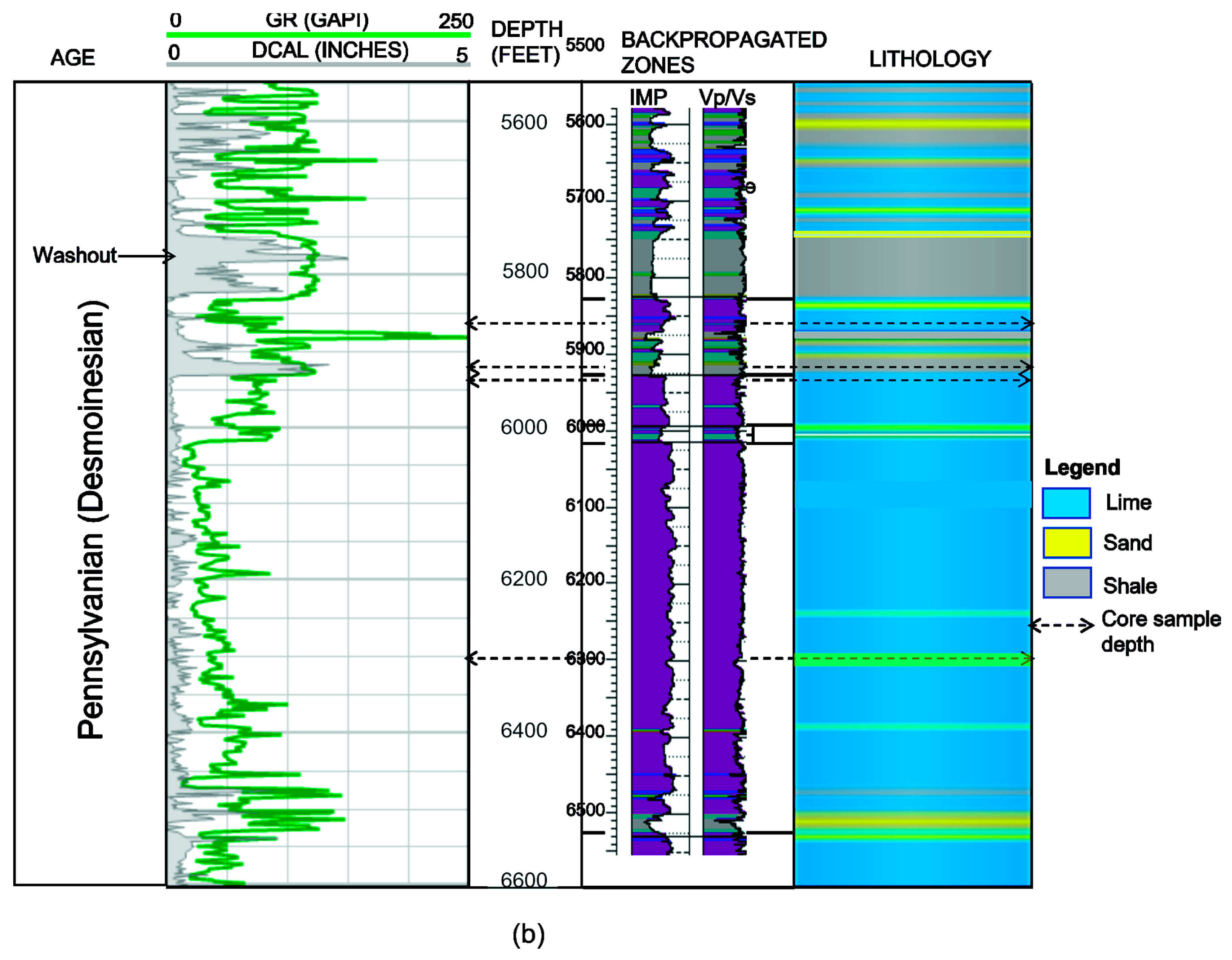
4.3. Petrophysical Inversion and Lithology Interpretation

We performed joint inversion of wireline logs to estimate mineralogical composition of the Strawn Group, an inversion approach in which we used an objective function that tries to reduce the difference between original and synthetic logs generated during the modeling process. Multi-mineralogy and porosity derived from the inversion approach show the vertical heterogeneity of the formation. Because we did not have complete log suites in every well, we used deterministic approaches to construct an overall lithology log for the Strawn Group in many wells.

4.4. Petrographic Analysis

We next integrated our results with petrographic thin-section analysis to validate the geophysically driven results. A total of 11 rotary cores (sidewall cores) were taken at selected depths within the Strawn Group in well 6, between 5842 ft (~1780 m) and 6546 ft (~1995 m) (Figure 2). Of these 11 samples, we present results from four locations—two samples representative of carbonates and the other two samples representative of a few siliciclastic zones, all of which are further discussed under Section 6.3—and Vp/Vs Ratios and petrographic analysis.

5. Results

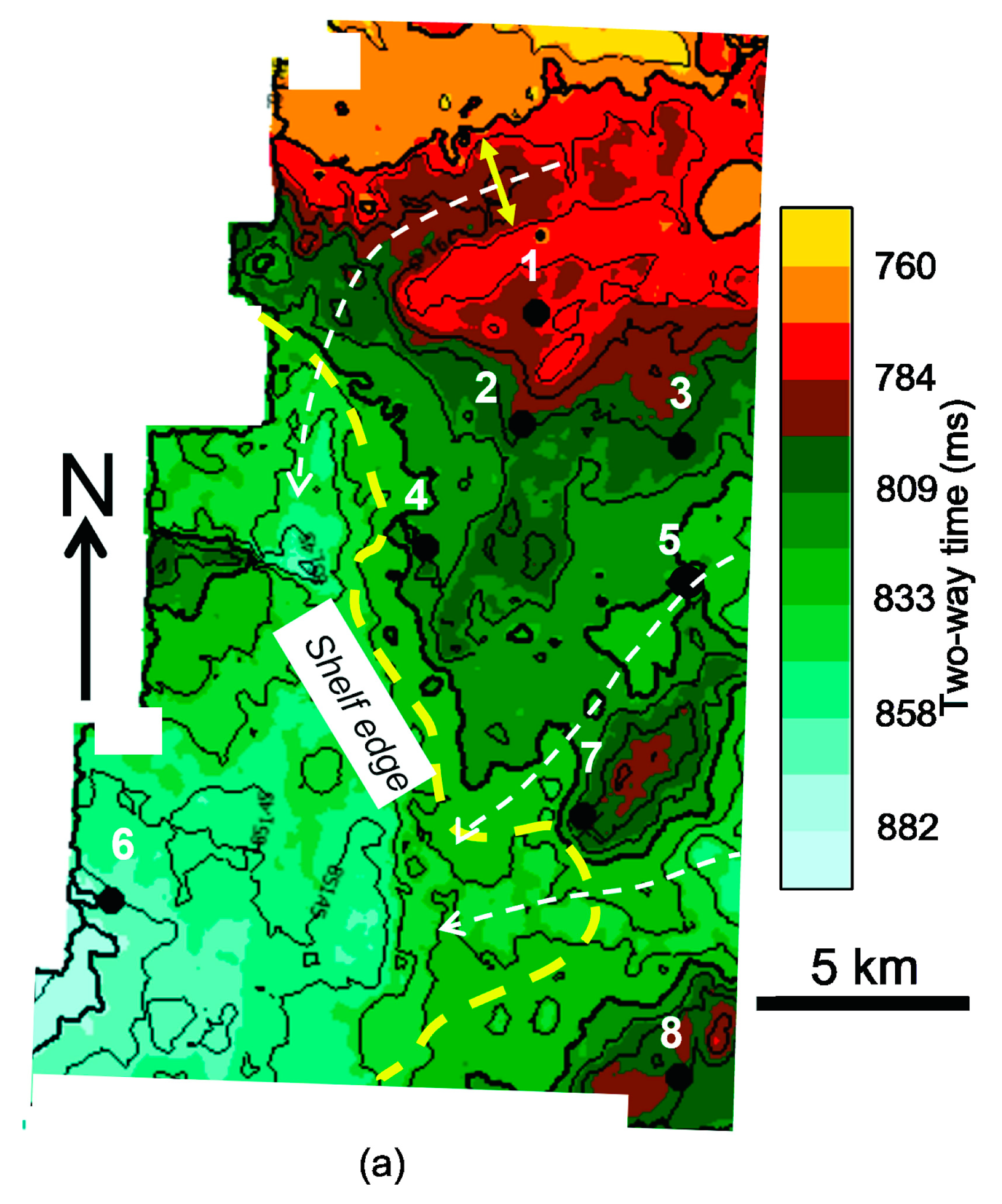
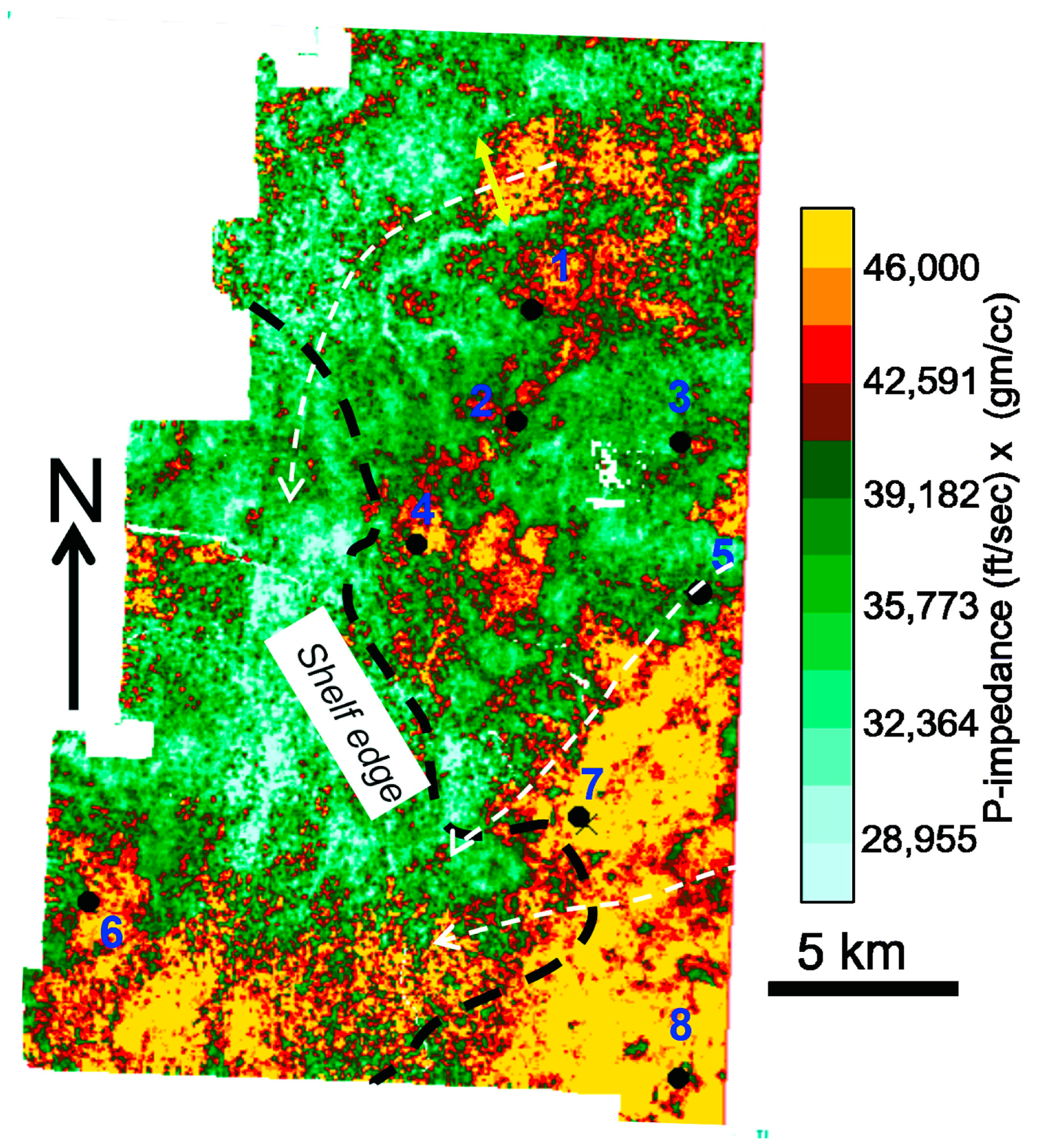
5.1. 3D Seismic Interpretation, Map at Top Strawn

A map at the top of Strawn Group shows that the landscape at the top Upper Strawn is composed of highs (topographic highs) and valleys, with the highs mostly located east of the shelf edge (dashed yellow line, Figure 7). Three major valleys trend northeast-southwest (dashed white arrows, Figure 7), through which sediments were routed into a northwest-southeast-trending basin. The valley at the extreme north appears to be an erosional gully entrenched within a topographic high composed of numerous small hills. At the yellow double-headed arrow location (Figure 7), the width of the valley is ~1.44 mi (~2.3 km) and its depth varies from ~45 ft (~14 m) in the east to ~140 ft (~43 m) in the west toward the shelf edge. The interpreted top Strawn horizon together with three other surfaces are displayed along seismic cross section A–A’ (Figure 7b). In this figure, two vertical faults (dashed-black lines) are shown. The rightmost fault has a downthrow to the northeast, while the leftmost fault downthrows to the southwest. The inserted black curve at the three well locations are gamma-ray log, while the other log is the interpreted lithology.

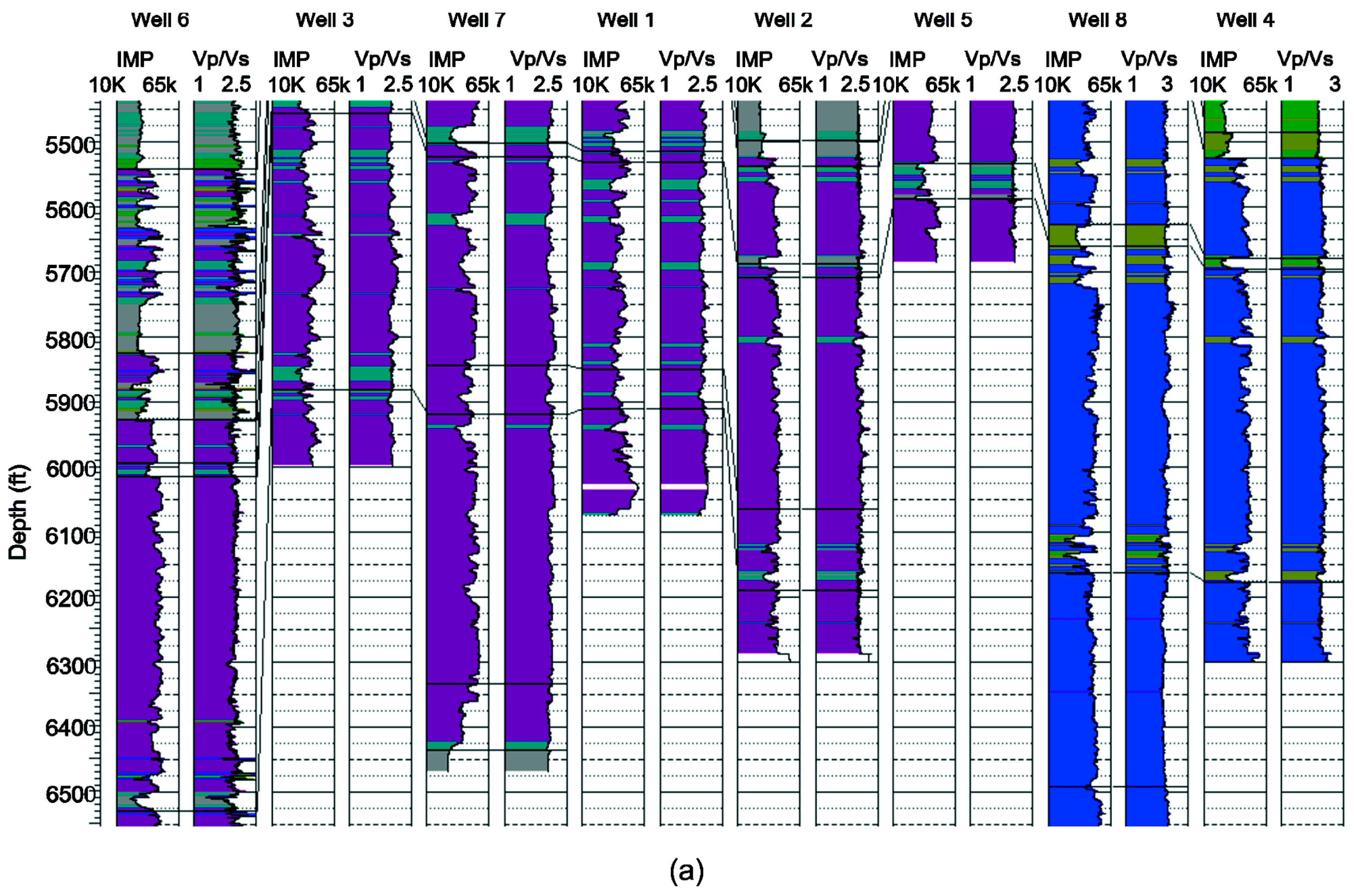
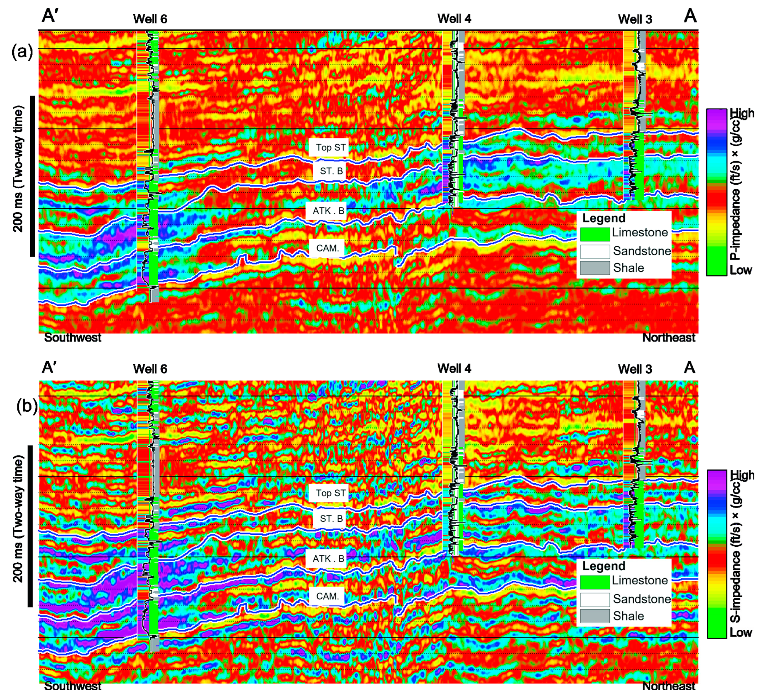
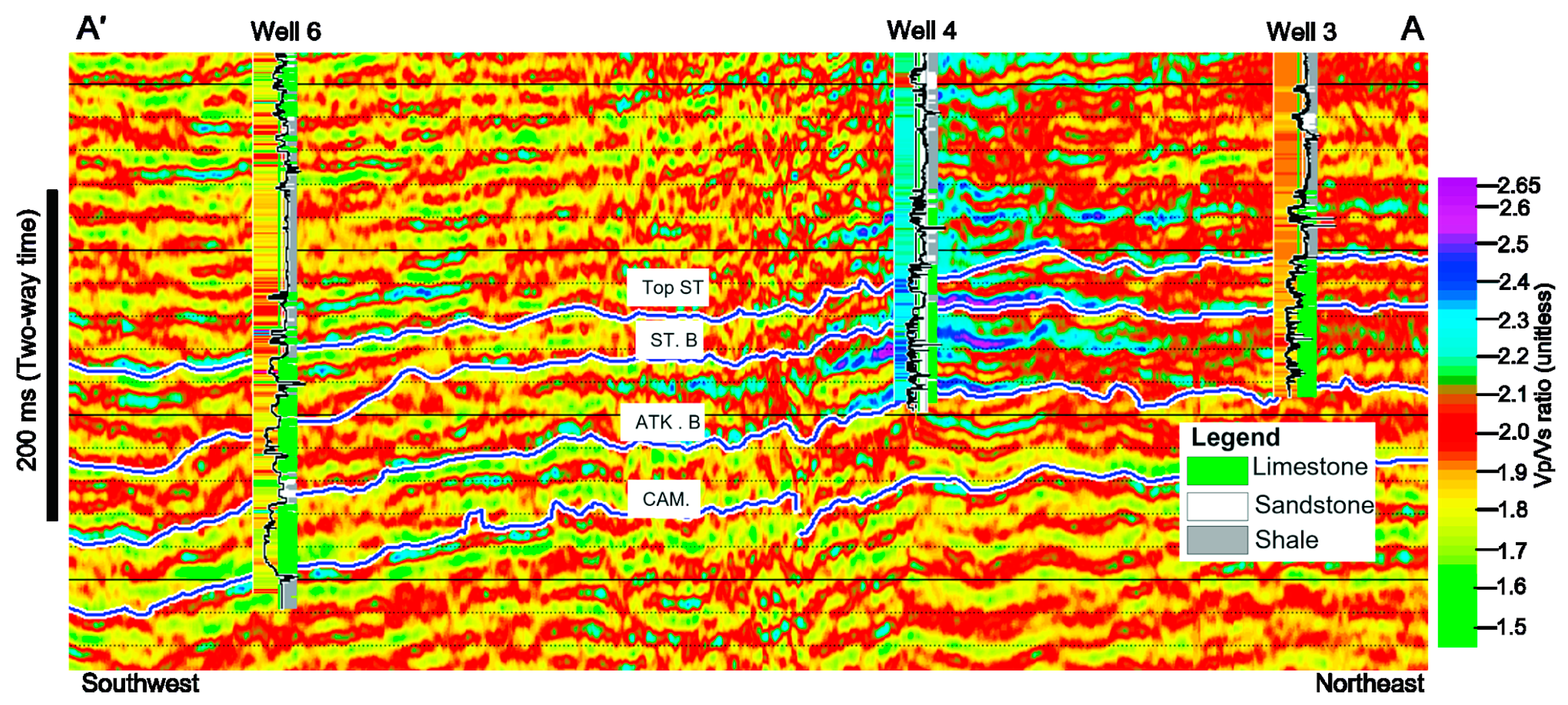
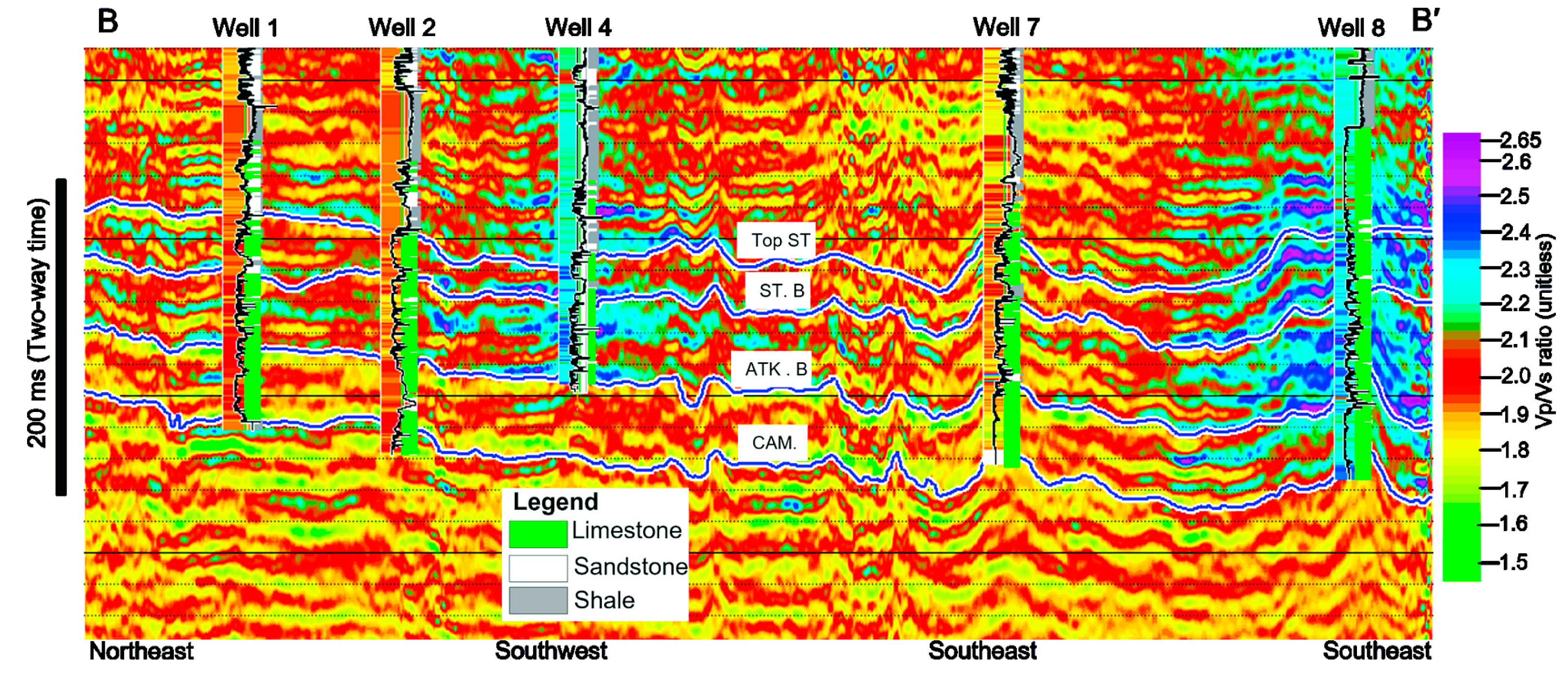
5.2. Simultaneous Seismic Inversion, Distribution of Elastic Properties

A cross section A–A’ of the inverted volumes connects three wells displaying P-wave and S-wave impedance sections (Figure 8a,b). In both sections, we inserted an impedance color log from the well bore, along with the lithology log, which is an interpretation of the wireline log showing three lithologies: carbonates (green), sandstones (white), and shale (gray). By incorporating the lithologic log into the inverted elastic sections, we demonstrated that the high-impedance zones correspond to carbonate, whereas the sandstone- and shale-rich zones (siliciclastics) have low impedance (Figure 8). The density section (Figure 9) is similar to P- and S-impedance in that the carbonates are of higher densities than the siliciclastics. In these three sections, a reasonable match occurs between the inverted data and the impedance color log. These figures also indicate that the Strawn Group in our area of investigation is composed mostly of carbonates interbedded with few very thin sandstone and shale zones. To examine the areal distribution of elastic properties and to infer lithologic distribution at the surface of the Strawn, we extracted these properties along the horizon map at the surface. Because the density and P- and S-impedances show similar results, we have presented only the P-impedance map extracted at the surface of the Strawn (Figure 10). This map shows that, although the remnant topographic highs (anticlinal structures) are characterized by high impedance and the valleys are filled with mostly low-impedance sediments, the widest valley that is located to the southeast between wells 7 and 8 is characterized by high impedance. In addition, the east part of the northeast-southwest-trending valley in the extreme north is characterized by high impedance, whereas the west half is characterized by low-impedance rocks (Figure 10).

5.3. Interpretation

On the basis of the seismic inversion and lithology logs, we interpreted the high-impedance zones to be composed of carbonates, whereas the low-impedance zones are interpreted to be composed of siliciclastic rocks. Note that, although the highs are composed mostly of high-impedance carbonates, the ridges bordering the northeast-southwest-trending valley to the north are characterized by low-impedance rocks, suggesting that the ridges are sandstone rich or that they are composed of porous carbonates. To interpret valley infills and northwest-southeast-trending basin sediments, we have displayed the Vp/Vs-ratio map at the surface of the Strawn (Figure 11). On this map, the shelf edge is shown as a combination of dashed red and white lines. Areas west of the shelf edge constitute valleys and the main northwest-southeast-trending basin. Vp/Vs-ratio values associated with the valleys and basin range from ~1.56 to 1.81 (Figure 11). The area east of the shelf edge can be divided into approximately three zones: (1) two main red zones (white outlines), (2) light-blue to dark-blue zones, and (3) dark-magenta zones with a few magenta zones. However, some scattered red zones lie within the light- and dark-blue zones that have a different range of Vp/Vs-ratio values and represent different lithologies and facies. The two red zones close to the shelf edge have high-Vp/Vs-ratio values ranging from ~2.05 to >2.49. The light-blue to dark-blue zones have values ranging from ~1.89 to 2.05, whereas the magenta to dark-magenta values range from ~1.74 to 1.89. To explain the lithology and facies distribution, we considered two cross sections (A–A’ and B–B’) of the Vp/Vs ratio volume (Figure 12 and Figure 13). Along cross section A–A’, we observed that, apart from well 4, the carbonate rocks (green) along the well bore (inserted lithology log and Vp/Vs ratio color log) at the wells 3 and 6 locations are characterized by low-Vp/Vs-ratio values ranging from 1.76 to ~1.93. In contrast, at the well 4 location, carbonate rocks are characterized by high-Vp/Vs-ratio values ranging from 2.06 to 2.65. The second cross section, B–B’, passes through wells 1 and 2, then runs southeast parallel to the shelf edge connecting wells 4, 7, and 8 (Figure 13). Note that, apart from wells 4 and 8, carbonate rocks (green) along the well bore (inserted lithology log and Vp/Vs color log) at the well locations are characterized by low-Vp/Vs-ratio values ranging from 1.76 to ~2.06. In contrast, at wells 4 and 8, the carbonate rocks are characterized by high-Vp/Vs-ratio values ranging from 2.06 to 2.65. These two wells are located at or close to the shelf edge, particularly well 4. Because of the associated depositional geometry of carbonate buildup at well 4 (Figure 12 and Figure 13), we interpreted the carbonate buildup to be a shelf-edge reef, herein referred to as reef #1. It terminates basinward because of a continuous increase in water depth, but builds gradually on the shelf and eastward before dying out. On the basis of the depositional geometry of the carbonate at well 8, we interpreted it to be a shelf-edge reef mound, herein referred to as reef #2. Cross section C–C’, connecting wells 4 and 5 (Figure 14), also shows that the carbonate buildup at well 4 is a shelf-edge reef. Here, Vp/Vs-ratio values associated with the carbonates at well 5 on the shelf are lower than those at well 4 (~1.86 to 1.93). In addition, we observed that in both the inverted-Vp/Vs-ratio section and inserted Vp/Vs ratio color log and lithology log, carbonate rocks in wells 1 and 2 located east of the shelf edge (Figure 11) have higher Vp/Vs values than do the carbonate rocks in well 7, which lies just east of the shelf edge on a carbonate high (Figure 11 and Figure 13), suggesting that wells 1 and 2 are in a different carbonate depositional environment and, thus, of a different facies from that in well 7. On the basis of the inserted Vp/Vs ratio color log and lithology log, we interpreted the dark- and light-blue, including the magenta areas east of the shelf edge, to be platform carbonates, whereas the pale-magenta to tan areas west of the shelf edge are slope and basin carbonates. Note the reasonable agreement between the Vp/Vs ratio color log and inverted section at the well locations.

6. Discussion

Because the Strawn Group found in our area of investigation is composed mostly of carbonates (near the shelf), we focused on carbonate facies variation and distribution on the basis of the Vp/Vs-ratio map, Vp/Vs-ratio cross sections, and cross plots. First, we considered results from the cross plots of Vp/Vs ratio versus impedance (Figure 4). In this figure, we observed two different Vp/Vs-ratio deposits: (1) high-Vp/Vs ratio and (2) low-Vp/Vs-ratio deposits.

6.1. High-Vp/Vs-Ratio Deposits

High-Vp/Vs-ratio deposits are typified by wells 4 and 8 (Figure 11 and Figure 13), which are within the shelf-edge reef environment, with well 4 lying within shelf-edge reef #1, whereas well 8 lies within shelf-edge reef #2 (Figure 11 and Figure 13). Further cross plots of Vp/Vs ratio versus porosity for well 8, representative of shelf-edge reef, show that the Vp/Vs ratio within shelf-edge reefs decreases as porosity increases (Figure 15). This observation conforms with laboratory experimental results [19], in which Vp/Vs ratio decreases as porosity increases when pore spaces are saturated with water. It also agrees with observations in the Scipio field [15], in which the Vp/Vs ratio decreases with an increase in porosity within the dolomitized zone. On the basis of observations [15,19], we interpreted the reefs to be relatively porous water-saturated carbonate mudstone.

6.2. Low-Vp/Vs-Ratio Deposits

Low-Vp/Vs-ratio deposits are typified by wells 1, 2, 3, 5, 6, and 7 and, on the basis of a Vp/Vs ratio map (Figure 11), these deposits can be separated into (1) moderately low Vp/Vs-ratio deposits typified by on-shelf wells 1, 2, 3, and 5 (Figure 11) and (2) extremely low Vp/Vs-ratio deposits represented by basinal and slope wells 6 and 7, respectively, shown along cross section D–D’ (Figure 16). Cross plots of Vp/Vs ratio versus porosity (color coded with impedance) for wells 3 representing the moderately low-Vp/Vs-ratio zone show an inverse trend, that is, the Vp/Vs ratio decreases as the porosity increases (Figure 17). Vp/Vs ratio values (Figure 17) vary from 1.75 to 2.05 and, in the case of the extremely low Vp/Vs ratio, cross plots at wells 6 and 7 (color coded with impedance) from the basin and slope environments (Figure 18) show that the gradient of the best-fit straight line to the plotted points is almost zero at 0.04, suggesting that the Vp/Vs ratio is almost constant at ~1.88. Nevertheless, the overall relationship is that the Vp/Vs ratio increases with increasing porosity. This observation contrasts with that of the relationship between the Vp/Vs ratio and the porosity seen in the reef and platform environments (this contrast is further examined in Section 6.3, Vp/Vs ratios and petrographic analysis). Although a few scattered high-Vp/Vs-ratio values occur in this zone, the dominant Vp/Vs-ratio values remain almost constant, dominated by values between 1.5 and 2 (Figure 18). The low-Vp/Vs-ratio values seen in wells 6 and 7 in the basin and slope areas suggest that the shear-wave velocity (Vs) is high, >½Vp, whereas the high Vp/Vs ratio (>2) observed in the reefs implies that Vs is low (<½Vp), further suggesting that reefs have more porous zones than do basin carbonates.

6.3. Vp/Vs Ratios and Petrographic Analysis

To determine the main cause of differences in the Vp/Vs ratio between reef carbonates, basinal carbonates, and those located on platform areas, we turned to results from complementary petrographic studies. Although we have no core data for reef carbonates, rotary core data were available for the Strawn group in well 6. In addition, petrographic data from conventional cores were available for wells 9 and 10 located outside the inversion area ~3.4 (~5.4) and 4.0 mi (~6.4 km) northeast of wells 8 and 3, respectively (Figure 11).

6.3.1. Vp/Vs Ratios and Well 6 Petrographic Analysis from Rotary Core

The first sample from well 6 came from a depth of 5855 ft (~1786 m), which is ~20 ft (~6.1 m) below the top of Strawn (double-headed dashed black arrow, Figure 19). After petrographic analysis, we found the bulk mineralogy of this sample to be 97.7% calcite, 1.2% dolomite, and 1.1% quartz. Core photographic and petrographic analysis showed that the rock sample at this depth is a massive packstone to wackestone containing abundant fine-grained peloids and moderate lime–mud matrix. Poorly sorted, it has a large allochem texture without encrusting species, suggesting a low-energy depositional environment such as near a sponge-dominant biomound. Because of the occurrence of abundant calcite recrystallization cements and replacements due to diagenesis, fractures have been resealed by calcite, although few remained opened (Figure 20a). Hence, the porosity of this sample is low at 0.4%.

The second core sample is from a shale-rich zone at a depth of 5925 ft (1806 m) (double-headed dashed black arrow, Figure 19). The sample is a deepwater highly burrowed, homogeneous mudstone. Petrographic studies showed that the dominant minerals are 60% clay, 30.7% quartz, and 7.7% feldspar. The major diagenetic process is pyrite replacement of grains, matrix, and organic materials. It is highly compacted, with no visible porosity (Figure 20b), and the few fractures have been replaced by pyrite.

The third core sample is from a depth of 5945 ft (1812 m) (double-headed dashed black arrow, Figure 19). The bulk mineralogy of this sample is 59.7% calcite, 24.8% quartz, and 9.5% clay. This rock sample is a spicule-rich bioclast packstone and mud-rich wackestone that was deposited in an outer-shelf environment. Petrographic analysis showed that, owing to diagenetic processes, siliceous sponge spicules and other skeletal grains have been replaced by authigenic calcite (Figure 20c). Hence, the porosity of this rock is low at 0.6%. Log analysis (Figure 19) revealed that the porosity at this sample is ~0. The occurrence of minor pyrite replacement of grains, matrix, and organic materials, as well as the presence of locally intense bioturbation, suggests a deepwater and low-energy depositional setting.

The fourth core sample is from a sandstone-rich zone at a depth of 6303 ft (~1921 m) (Figure 19). Petrographic studies revealed that the bulk mineralogy is 98.7% quartz and 1.3% calcite. Results also showed that associated carbonate mud and shales have been silicified by microquartz owing to diagenesis. The sandstone is highly fractured (Figure 20d) and the silicified sponge spiculite of deepwater origin has been subjected to deep burial. Analysis further revealed that fractures such as those stained red (Figure 20d) that were generated during deep burial have been resealed by microquartz and calcite. Hence, the rock has no visible porosity, that is, porosity is low. The low or near-zero porosity at this depth is also confirmed by log analysis (Figure 19).

In summary, the Strawn Group interval penetrated by well 6 is mostly a deepwater-deposited carbonate-dominated rock. It is highly compacted with little or no porosity. In this type of rock, although Vp/Vs ratio is low and remaining almost constant because the rock is tight, it increases gradually as porosity increases [18] (Figure 18). Because the Vp/Vs ratio is low, mostly between 1.5 and 2, S-wave velocity Vs is high, greater than half Vp (Vs > ½Vp). Both petrographic studies and log-analysis results (Figure 19) show that porosity is low.

6.3.2. Vp/Vs Ratios and Wells 9 and 10 Petrographic Analysis from Conventional Core

Strawn Group carbonates at wells 9 and 10 are composed of inner-ramp shallow-water to middle-ramp moderate deepwater to outer-ramp deepwater deposits [29]. Although we cannot provide all the details of these workers’ results here in this paper, note that the lithofacies described by them consist of (1) bioclast grainstones to mud-lean packstones, (2) bioclast wackestones to mud-rich packstones, (3) intraclastic rudstones, (4) dark bioclast packstones to wackestones, (5) sandy bioclast packstones, and (6) black mudrocks [29], which are all products of alternating sea levels (transgression and regression). Fluctuation of sea levels also occurred frequently during the Pennsylvanian [29]. As such, during sea-level falls (regression), shelf-edge reefs and shelf (i.e., platform) carbonates were exposed to the influence of meteoric waters and, because of this exposure, diagenetic processes that transformed the carbonates occurred, leading to the dissolution and leaching of the rocks. These processes in turn led to the abundance of vugs and molds within thick packstone and wackestone intervals in wells 9 and 10 [29]. These authors also observed leaching of the matrix in some cases, leading to the development of micro-vugs or enhanced matrix pores. The overall effect of the abundance of vugs and intragranular pores within these carbonates was the increase in porosity. Thus, compared with the carbonates in well 6, which were mostly in deep water, carbonates in wells 9 and 10 would be more porous. Photomicrographs of intragranular pores and vugs from wells 9 and 10, respectively, of the core samples are shown in (Figure 21a,b). A photomicrograph of the porous carbonates of well 9 and the tight nonporous carbonate of well 6 emphasizes the differences between the two carbonate types (Figure 22). Although no core data of shelf-edge reefs #1 and #2 were available, because well 8 is located on top of shelf-edge reef #2 and ~3.4 mi (~5.4 km) southwest of well 9, we inferred that reef #2 would have pore spaces (vugs, molds, and intragranular pores) similar to those observed in well 9. Note that, given the geometry of reef #2 (Figure 16), the outline of reef #2 might be approximately circular (dashed-blue outline, Figure 11), suggesting that a section of reef #2 (Figure 11) is just a small part of the entire reef and that well 9 was probably drilled at the edge of reef #2. Similarly, although no core data were available for platform wells 1, 2, 3, or 5, because these wells lie on the shelf—as in well 10, which is ~4 mi (~6.4 km) northeast of well 3 (Figure 11)—we inferred that these wells would have porosities similar to that of well 10 (Figure 21b). Additionally, because the platform carbonates are probably more porous than the basinal carbonates in well 6, they have higher Vp/Vs ratios. However, as demonstrated in Figure 11, Figure 12, Figure 13 and Figure 14, reefs (e.g., wells 4 and 8) have higher Vp/Vs ratios than those of platform carbonates (e.g., wells 1, 2, 3, and 5), implying that reef carbonates might be more porous than shelf and basin carbonates. The reason for this difference in physical property is captured in a schematic depositional model (Figure 23), which shows that during sea-level fall reefs are topographically higher than basinal areas; they are therefore more exposed to meteoric waters, causing them to become vuggier than basinal and platform carbonates, owing to dissolution and leaching. However, a comparison between the cross plots of Vp/Vs ratios versus porosities for well 8, platform well 3, and the basinal wells 6 and 7 (Figure 15, Figure 17 and Figure 18), respectively, shows that the reefs, platform, and basinal carbonates have the same porosity range of <16%. Because both the reef carbonates and the basinal carbonates have the same porosity range, it means that depositional environment and associated diagenetic processes are more likely to be the main cause of the differences in the Vp/Vs ratio than porosity, that is, the difference in Vp/Vs ratios among the carbonate facies is not entirely due to porosity but to a combination of other factors. As noted by [30], acoustic velocities in carbonate rocks are highly affected by porosity, texture, pore shapes, pore aspect ratio, and pore fluids. Thus, carbonate rocks whose pores are predominantly vuggy or moldic, have a different acoustic velocity from those with predominantly intercrystalline and or interparticle pores even for the same porosity [31]. In addition, [19] pointed out that, when fluid is present in pores shaped differently from thin cracks (e.g., tubes, spherical pores, polygonal grain junctions, or vugs), the change in the Vp/Vs ratio with increasing fluid saturation-saturated porosity is not necessarily an increase in the Vp/Vs ratio; instead of increasing, the VP/Vs ratio decreases with an increase in porosity. This is the situation observed in the reef and shelf environments, suggesting that pore shapes in these carbonates are different from those in the slope and basin environments. Consequently, the Vp/Vs ratio would be a better tool to distinguish the different carbonate facies depositional environments than porosity. We thus inferred that the reef carbonates have higher Vp/Vs ratios than do the shelf and basinal carbonates, because they have been affected by different diagenetic processes that changed their pore geometry, that is, for the Strawn Group in the study area, the Vp/Vs ratio of reef carbonates > the Vp/Vs ratio of platform carbonates and >the Vp/Vs ratio of slope and basin carbonates.

7. Conclusions

The Strawn Group in the study area is composed of carbonates, sandstone, and shales, but it is dominated by carbonates. In a mixed carbonate and siliciclastic setting, carbonates stand out as topographic highs because of their denser nature. By using simultaneous seismic inversion and wireline logs to investigate the Strawn Group and also by the cross plotting of Vp/Vs ratio versus porosity, we found that the carbonates can be separated into three types: (1) high-Vp/Vs-ratio shelf-edge carbonates, in which the Vp/Vs ratio decreases linearly as porosity increases; (2) moderately low Vp/Vs ratio platform carbonates, in which the Vp/Vs ratio also decreases as porosity increases; (3) extremely low Vp/Vs-ratio basin carbonates, in which the gradient of the best-fit straight line to the plotted points is almost zero at 0.04, suggesting that the Vp/Vs ratio is almost constant at ~1.88 (the Vp/Vs ratio nevertheless increases with increasing porosity). In addition, we found that changes in Vp/Vs ratios in carbonate rocks are more likely to be influenced by depositional environment than porosity. Therefore, the Vp/Vs ratio would be a better tool for distinguishing different carbonate facies. We also found that on the basis of the Vp/Vs ratio, we could infer (1) valley and basin infills to be a mixture of eroded carbonates and siliciclastic rocks; (2) some of the valleys to be ≤140 ft (43 m) deep and ≤1.44 mi (2.3 km) wide; (3) high ridges to the north to be composed of low-impedance and low-density rocks, suggesting that the rocks are probably sandstone and shales.

Finally, we would like to point out that, although prestack simultaneous seismic inversion method is a powerful tool, the accuracy is limited by poor well-to-seismic tie, noisy seismic data, poor log quality, seismic resolution, and a limited number of wells.

References

- Payros, A.; Pujalte, V. Calciclastic submarine fans: An integrated overview. Earth Sci. Rev. 2008, 86, 203–246. [Google Scholar] [CrossRef]
- Chiarella, D.; Longhitano, S.G.; Tropeano, M. Types of mixing and heterogeneities in siliciclastic-carbonate sediments. Mar. Pet. Geol. 2017, 88, 617–627. [Google Scholar] [CrossRef] [Green Version]
- Tucker, M.E. Mixed Clastic–Carbonate Cycles and Sequences: Quaternary of Egypt and Carboniferous of England. Geol. Croat. 2003, 56, 19–37. [Google Scholar] [CrossRef]
- Cleaves, A.W. Strawn and Canyon Depositional Systems, Sedimentation History and Exploration Models for the Concho Platform-Eastern Shelf of North-Central Texas. Abilene Geol. Soc. 1983, pp. 1–83. Available online: https://archives.datapages.com/data/abilene/data/strawn_canyon83/Strawn_Canyon_83.htm (accessed on 20 October 2022).
- Cleaves, A.W.; Erxleben, A.W. Upper Strawn and Canyon cratonic depositional systems of Bend Arch, north-central Texas. In Transactions of the AAPG Southwest Section Regional Meeting; McNulty, C., McPherson, J.C., Eds.; Fort Worth Geological Society: Fort Worth, TX, USA, 1985; pp. 27–46. [Google Scholar]
- Boring, T.H. Upper Strawn (Desmoinesian) carbonate and clastic depositional environments, southeast King County, Texas. In Petroleum Reservoir Geology in the Southern Midcontinent, 1991 Symposium; Johnson, K.S., Campbell, J.A., Eds.; University of Oklahoma: Norman, CA, USA, 1993; pp. 195–198. [Google Scholar]
- Russell, B.H.; Hampson, D.; Bankhead, B. An inversion primer. CSEG Rec. Spec. Issue 2006, 31, 96–103. [Google Scholar]
- Yenwongfai, H.D.; Mondol, N.H.; Faleide, J.I.; Lecomte, I.; Leutscher, J. Pre-stack inversion and multiattribute analysis for porosity, shale volume, and sand probability in the Havert Formation of the Goliat field, southwest Barents Sea. Interpretation 2017, 5, SL69–SL87. [Google Scholar] [CrossRef] [Green Version]
- Maxan, J. Variation of density with rock type, depth, and formation in the Western Canada Basin from density logs. Geophysics 1980, 15, 1061–1076. [Google Scholar] [CrossRef]
- Braun, J.; Simon-Labric, T.; Murray, K.E.; Reiners, P.W. Topographic relief driven by variations in surface rock density. Nat. Geosci. 2014, 7, 534–540. [Google Scholar] [CrossRef]
- Tatham, R.H.; McCormack, M.D. Multicomponent Seismology in Petroleum Exploration: Investigations in Geophysics; SEG: Houston, TX, USA, 1985; Volume 6, 248p. [Google Scholar]
- Christensen, N.I. Poisson’s ratio and crustal seismology. J. Geophys. Res. 1996, 101, 3139–3156. [Google Scholar] [CrossRef]
- Robertson, J.D. Carbonate porosity from S/P traveltime ratios. Geophysics 1987, 52, 1346–1354. [Google Scholar] [CrossRef]
- Pardus, Y.; Conner, J.; Schuler, N.; Tatham, R. Vp/Vs, Lithology in Carbonate Rocks: A Case History in the Scipio Trend in Southern Michigan; SEG Technical Program Expanded Abstracts 1990; Society of Exploration Geophysicists: Houston, TX, USA, 1990; pp. 169–172. [Google Scholar]
- O’Connell, R.J.; Budiansky, B. Seismic velocities in dry and saturated cracked solids. J. Geophys. Res. 1974, 79, 5412–5426. [Google Scholar] [CrossRef]
- Takei, Y. Effect of pore geometry on VP/VS: From equilibrium geometry to crack. J. Geophys. Res. 2002, 107, ECV6-1–ECV6-12. [Google Scholar] [CrossRef]
- McCormack, M.D.; Justice, M.G.; Sharp, W.W. A stratigraphic interpretation of shear and compressional wave seismic data for the Pennsylvanian Morrow formation of southeastern New Mexico. AAPG Memoir 1985, 39, 224–239. [Google Scholar]
- Lee, M.W.; Norton, G.A.; Groat, C.G. Velocity Ratio and Its Application to Predicting Velocities; US Department of the interior, US Geological Survey: Reston, VA, USA, 2003; Volume 2197, pp. 1–15. Available online: https://pubs.usgs.gov/bul/b2197/B2197-508.pdf (accessed on 10 November 2022).
- Watanabe, T. Effects of water and melt on seismic velocities and their application to characterization of seismic reflectors. Geophysics. Res. Lett. 1993, 20, 2933–2936. [Google Scholar] [CrossRef]
- Hosseini-Fard, E.; Roshandel-Kahoo, A.; Soleimani-Monfared, M.; Khayer, K.; Ahmadi-Fard, A.R. Automatic seismic image segmentation by introducing a novel strategy in histogram of oriented gradients. J. Pet. Sci. Eng. 2022, 209, 109971. [Google Scholar] [CrossRef]
- Hosseini, A.; Ziaii, M.; Rouhani, A.K.; Roshandel, A.; Gholami, R.; Hanachi, J. Artificial intelligence for prediction of porosity from seismic attributes: Case study in the Persian Gulf. Iran. J. Earth Sci. 2011, 3, 168–174. [Google Scholar]
- Al Salem, O.B. The Subsidence Evolution of the Fort Worth Basin in North-Central Texas. Master’s Thesis, The University of Texas at Arlington, Arlington, TX, USA, 2014. Available online: https://rc.library.uta.edu/uta-ir/bitstream/handle/10106/24705/AlSalem_uta_2502M_12753.pdf?sequence=1&isAllowed=y. (accessed on 3 December 2022).
- Marshak, S. Earth: Portrait of a Planet; WW Norton & Company: New York, NY, USA, 2001; pp. 528–529. ISBN 0-393-97423-5. [Google Scholar]
- Cleaves, A.W. Sequence stratigraphy, systems tracts, and mapping strategies for the subsurface Middle and Upper Pennsylvanian of the eastern shelf. In AAPG Southwest Section, Regional Meeting, Transactions; Crick, R.E., Ed.; Fort Worth Geological Society: Fort Worth, TX, USA, 1993; pp. 26–42. [Google Scholar]
- Cleaves, A.W. Sequence stratigraphy and reciprocal sedimentation in Middle and Late Pennsylvanian carbonate-bank systems, eastern shelf of the Midland Basin, north-central Texas. In Platform Carbonates in the Southern Midcontinent; Johnson, K.S., Ed.; University of Oklahoma: Norman, OK, USA, 2000; Volume 101, pp. 227–257. [Google Scholar]
- Hampson, D.; Russell, B.; Bankhead, B. Simultaneous Inversion of Pre-Stack Seismic Data; SEG Technical Program Expanded Abstracts 2005; Society of Exploration Geophysicists: Houston, TX, USA, 2005; pp. 1633–1636. Available online: https://library.seg.org/doi/epdfplus/10.1190/1.2148008 (accessed on 30 December 2022).
- Ma, X. Simultaneous inversion of prestack seismic data for rock properties using simulated annealing. Geophysics 2002, 67, 1877–1885. [Google Scholar] [CrossRef]
- Fatti, J.; Smith, G.; Vail, P.; Strauss, P.; Levitt, P. Detection of gas in sandstone reservoirs using AVO analysis: A 3D Seismic Case History Using the Geostack Technique. Geophysics 1994, 59, 1362–1376. [Google Scholar] [CrossRef]
- Fu, Q.; Ambrose, W.A. Lithofacies and diagenetic features of Strawn carbonates in the subsurface of North-Central Texas: Implications to controls on reservoir quality. GCAGS 2020, 9, 115–132. [Google Scholar]
- Weger, R.J.; Eberli, G.P.; Baechle, G.T.; Massaferro, J.L.; Sun, Y.F. Quantification of pore structure and its effect on sonic Velocity and permeability in carbonates. AAPG Bull. 2009, 93, 1297–1317. [Google Scholar] [CrossRef]
- Rossebo, O.H.; Brevik, I.; Ahmadi, G.R.; Adam, L. Modeling of acoustic properties in carbonate rocks: SEG Expanded Abstracts. Soc. Explor. Geophys. 2005, 24, 1505–1508. [Google Scholar]
Disclaimer/Publisher’s Note: The statements, opinions and data contained in all publications are solely those of the individual author(s) and contributor(s) and not of MDPI and/or the editor(s). MDPI and/or the editor(s) disclaim responsibility for any injury to people or property resulting from any ideas, methods, instructions or products referred to in the content. |
© 2023 by the authors. Licensee MDPI, Basel, Switzerland. This article is an open access article distributed under the terms and conditions of the Creative Commons Attribution (CC BY) license (https://creativecommons.org/licenses/by/4.0/).
Share and Cite
Ogiesoba, O.C.; Bhattacharya, S.; Karakaya, S.; Cortez, T. Prestack Seismic Velocity Ratio Evaluation of a Mixed Siliciclastic–Carbonate Formation: Case Study from the Strawn Group on the Eastern Shelf Texas. Energies 2023, 16, 2037. https://doi.org/10.3390/en16042037
Ogiesoba OC, Bhattacharya S, Karakaya S, Cortez T. Prestack Seismic Velocity Ratio Evaluation of a Mixed Siliciclastic–Carbonate Formation: Case Study from the Strawn Group on the Eastern Shelf Texas. Energies. 2023; 16(4):2037. https://doi.org/10.3390/en16042037
Chicago/Turabian StyleOgiesoba, Osareni C., Shuvajit Bhattacharya, Sarp Karakaya, and Trey Cortez. 2023. "Prestack Seismic Velocity Ratio Evaluation of a Mixed Siliciclastic–Carbonate Formation: Case Study from the Strawn Group on the Eastern Shelf Texas" Energies 16, no. 4: 2037. https://doi.org/10.3390/en16042037