1. Introduction
Current policies of the European Union and national governments are strongly pushing the transition to local zero-emission mobility based on electric vehicles (EVs). This is being followed by continued growth in the number of circulating electric vehicles. Therefore, we are witnessing a rapid and widespread development of the necessary charging infrastructure. The simultaneous global push toward energy transition leads to accompanying the installation of charging systems with the installation of photovoltaic and storage systems for optimal energy management. This is making demand forecasting an essential topic of strong interest.
On one hand, for the charging infrastructure providers, the forecasting of user energy consumption is essential to estimate possible revenues and losses to assess the cost-effectiveness of the installations [
1,
2]. On the other hand, for the grid operators, the forecasting of the power required for EV charging is mandatory to quantify the effects on the power grid management and stability [
3,
4,
5,
6]. Predicting the EV charge power profiles allows effective charging management strategies [
7] and the optimal integration of EVs with the electrical grid, storage systems, and renewable sources [
8,
9,
10,
11].
However, power forecasting in this context is still challenging due to several reasons. The current number of EVs is still statistically not representative to derive a robust model based on the available data [
12]. Moreover, despite the general continuous growth, in some countries like Italy, the number of new EV registrations is experiencing an unexpected decrease [
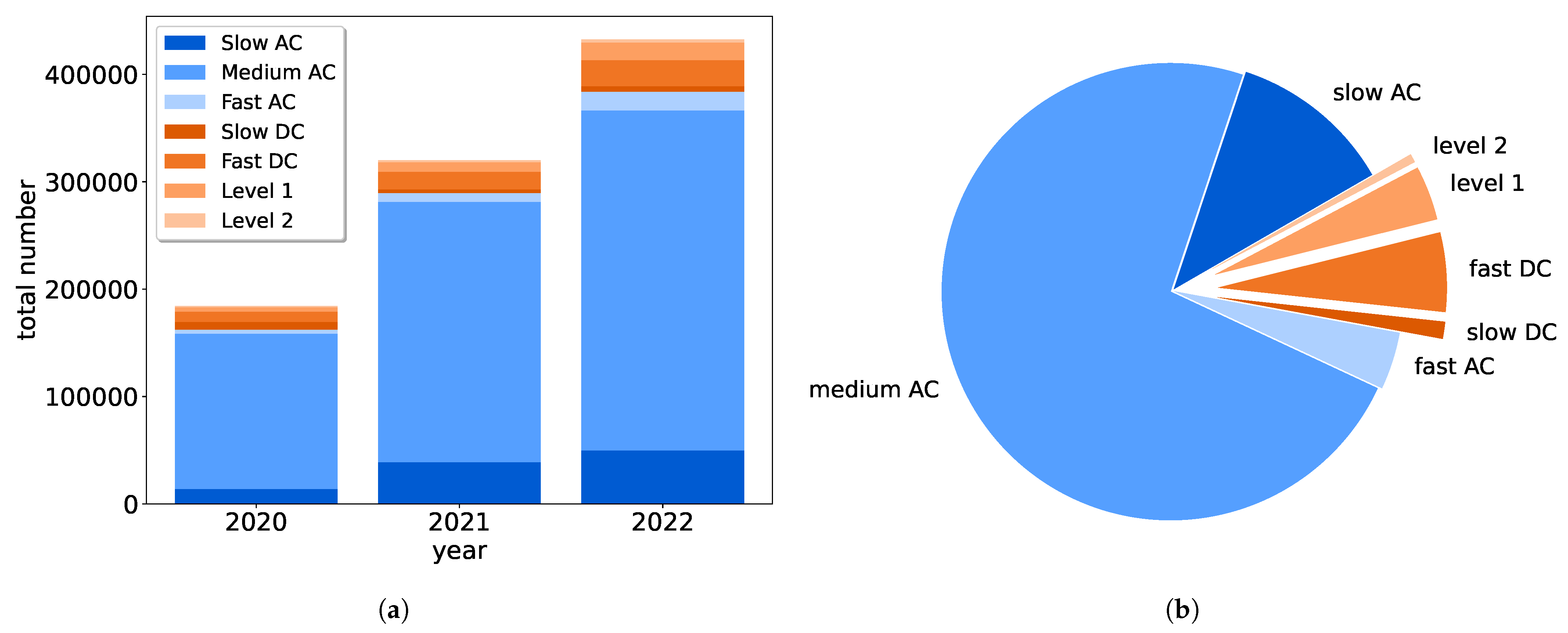
13]. Added to this is the fact that, the charging power profile is highly dependent on many different factors. The power level of the charging can vary in a wide range. The most common value is 22 kW for AC charging points (CPs) [
14], but it can reach hundreds of kW in the DC stations [
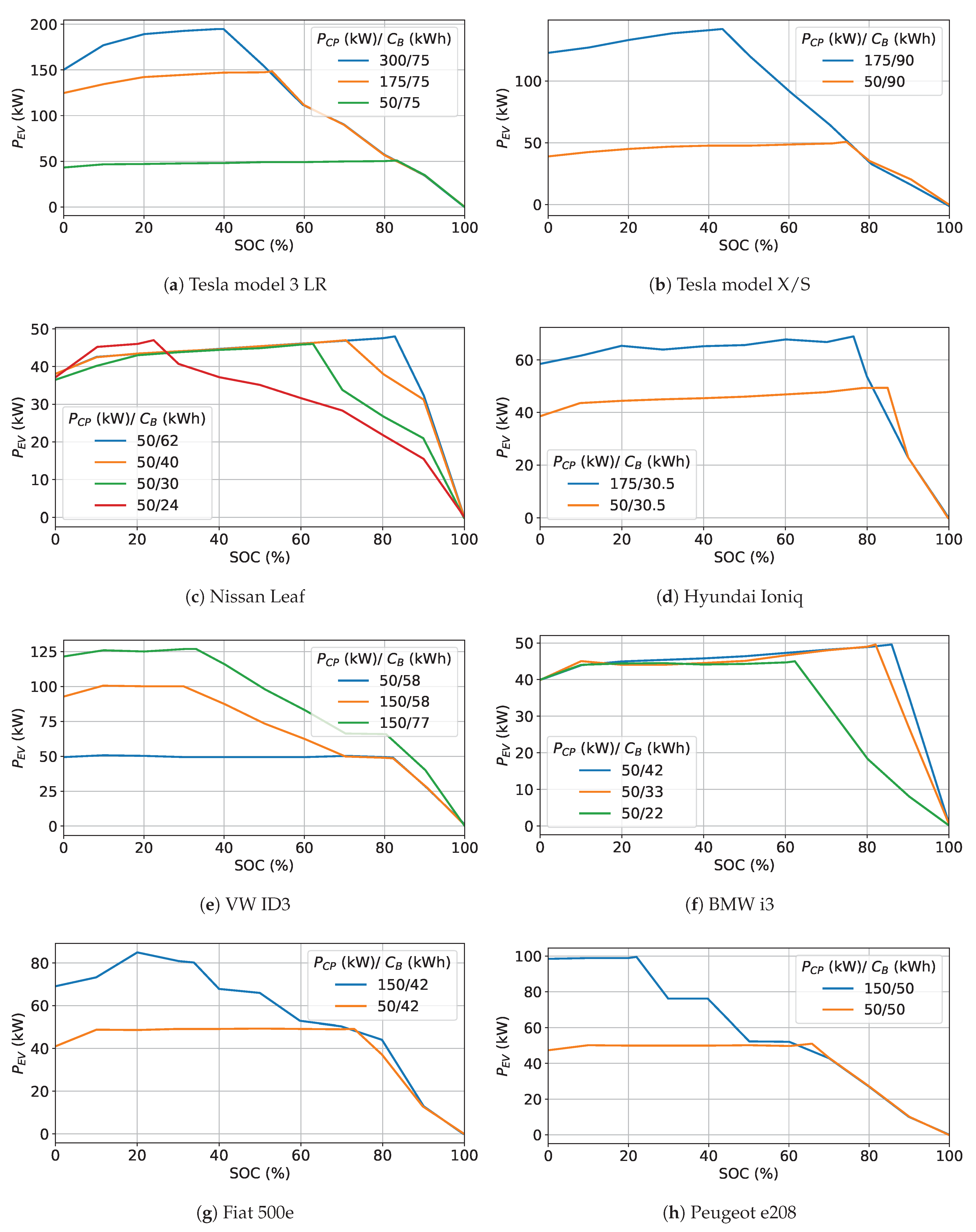
15]. However, the effective use of the available power level can vary among the different EV manufacturers and models [
16]. For example, the Renault ZOE can charge up to 46 kW in DC, while the Renault Twingo cannot exceed the 22 kW exclusively in the AC mode. The Tesla Model Y can achieve a 250 kW DC peak power during the charge. Eventually, this power level is not constant during the whole charging process. The charge of lithium batteries is typically carried out by means of the constant current-constant voltage (CC-CV) charging protocol [
17]. This protocol involves a reduction in the charging power during the final stage of charging to preserve the state of health of the battery. For this reason, the resulting power profile is discontinuous. Moreover, the profile of absorbed power varies in relation to many other factors such as the battery technology, the onboard charger, or the adopted battery management system [
18].
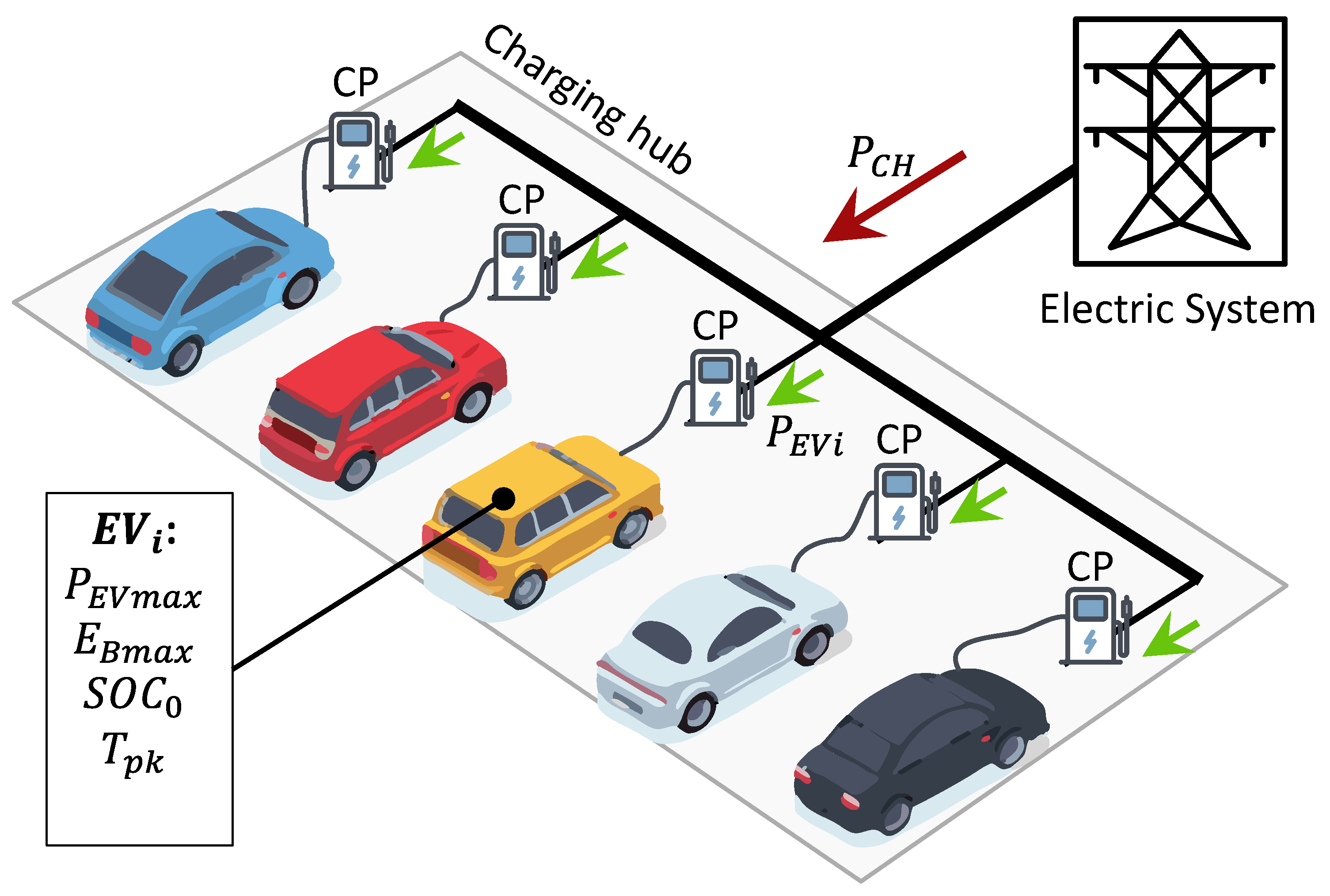
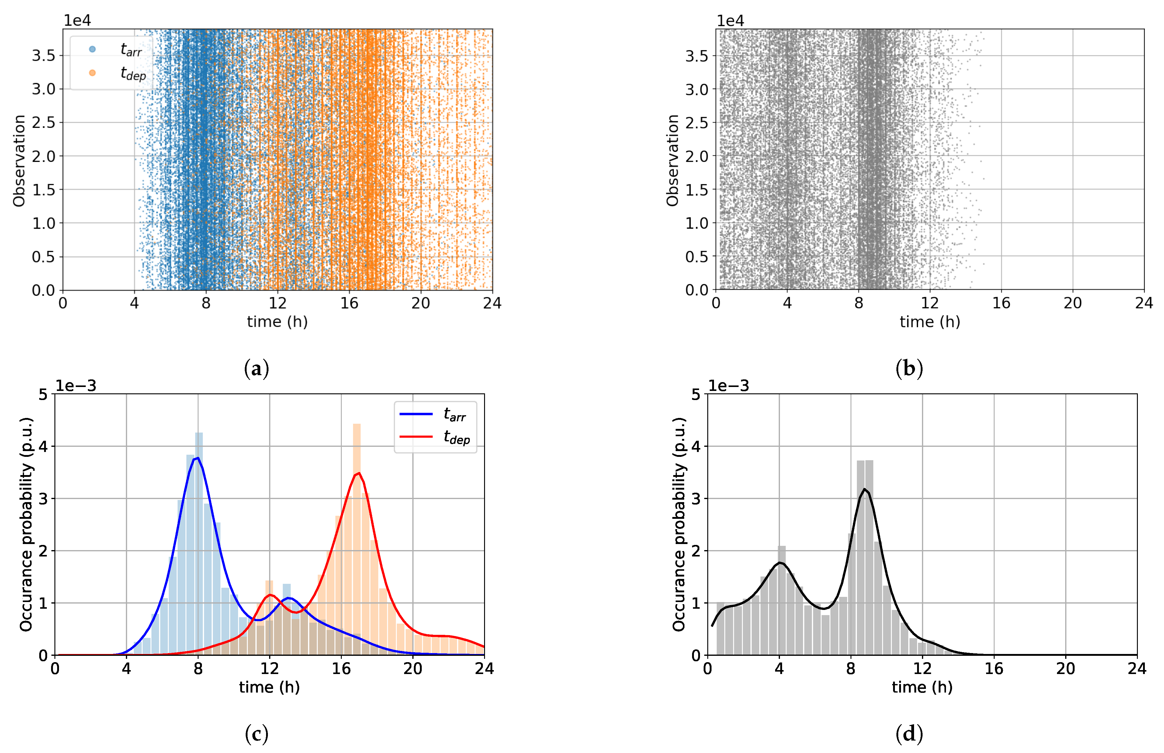
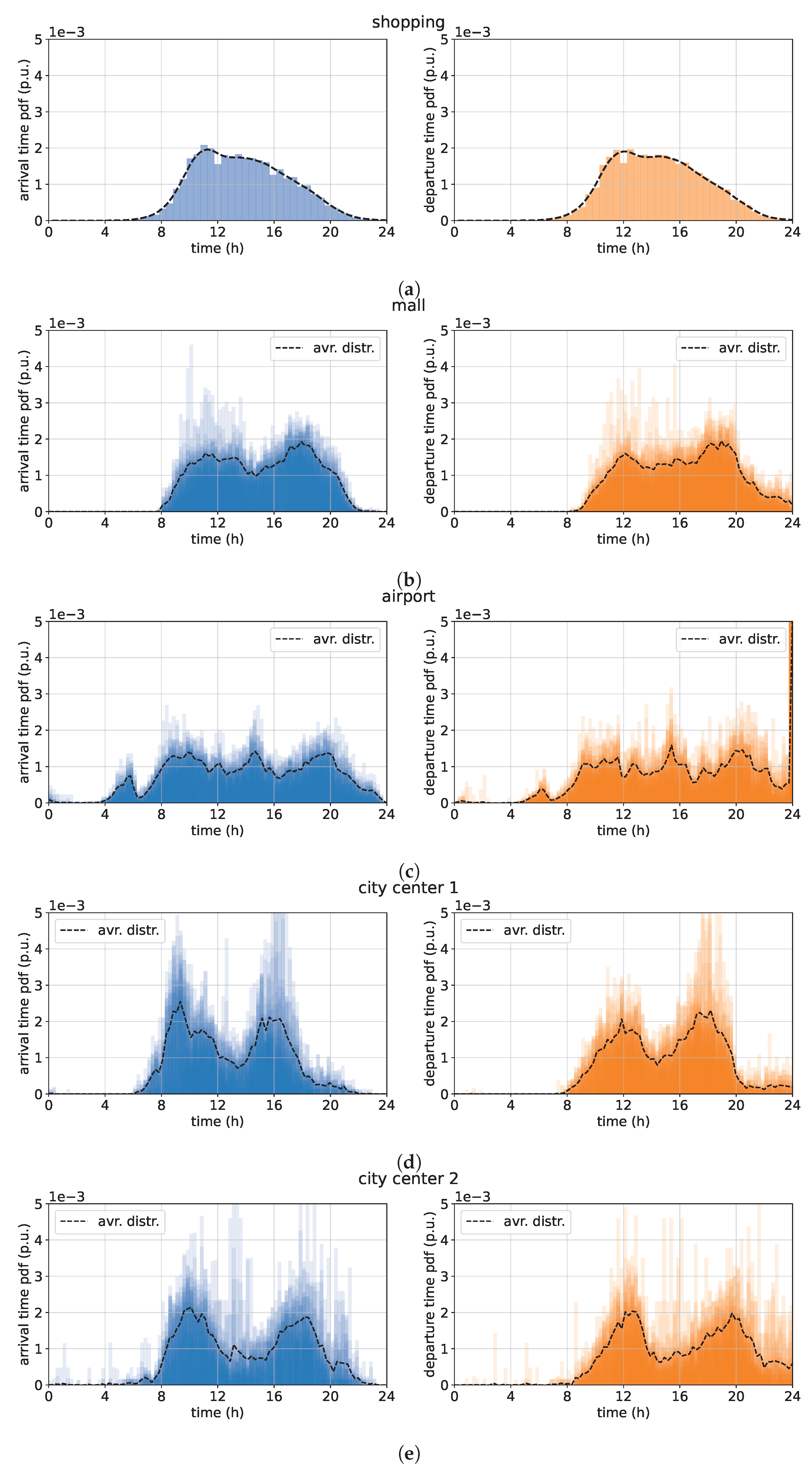
In the case of charging hubs (CHs), the whole absorbed power profile is in turn dependent on many other factors related to the considered scenario and the users’ behavior. The arrival times distribution of a CH of a working place parking lot typically presents a peak around the first-morning hours while, in a CH of a shopping area, this peak typically occurs around the evening. Finally, the energy demand of each CH is influenced by other factors like the state of charge (SOC) of the battery at the beginning of the charge, and the duration of parking (i.e., the time the CP remains occupied).
Several works about EV charging parameters forecasting can be found in the literature. Authors in [
19] adopted Bayesian inference methods with convolution to forecast the daily charging pattern of an EV fleet. This work only considers the 3 kW household power level, then results can not be applied to public CH in different parking lot scenarios, charging station power levels, and EV models. A day-ahead Bayesian deep learning forecasting method was proposed in [
20]. The objective was to capture the uncertainties in EV charging forecasting by adopting Bayesian theory and neural networks. In [
21], a forecasting method based on multi-source data and prospect theory was presented. The travel behaviour of private electric vehicles and taxi owners was considered along with the roads’ velocity and network. Authors in [
22] compared four different deep learning methods for a real case in Marocco to predict charging demand of an EV station. In [
23], a data-driven approach using machine learning regression methods is adopted for a public charging station. In [
24], historical data was clustered based on EV user behaviour and the corresponding probability density functions were derived. Three main parameters were considered, i.e., arrival time, charging duration and average power. These works, which are mainly based on charging data analysis, don’t provide a method able to take into account the single session charging power as a function of the time. Moreover, charging infrastructure and EV characteristics (such as initial/final state of charge, maximum power capability, battery capacity etc.) were not considered. Finally, authors in [
8] provide a forecasting method based on a statistical model of the arrival and departure time of the users. Although this method calculates the power consumed by each connected vehicle as a function of time, only 22 kW AC charging points are considered, and only a single parking scenario (i.e., a metal-working company) was analyzed. To the best of authors’ knowledge no papers provide a charging forecasting method based on specific EV and CH infrastructure characteristics, different urban scenarios, and real charging power profiles.
The proposed work aims to fill this gap at both single charging point and total charging hub level by considering multiple approaches. The users’ behavior is modeled through a statistical-based approach in which arrivals, departures, and charging durations are predicted based on the specific patterns related to the considered scenario. The distribution of the EV battery SOCs at the beginning of the charge is based on a probabilistic analysis of specific consumption and distances traveled before the charging event of each vehicle. A machine-learning-based approach is used to develop a battery charging behavioral model (BCBM). The BCBM is able to emulate the charging power profile of different EV models as a function of the battery SOC and the power rating of the CP to which the EV is connected. Based on custom input settings that describe the CH charging station characteristics, the expected number of EVs, and the operating scenario, the resulting forecasting algorithm evaluates the charging power profile of each EV and the SOC evolution of each EV during the whole period in which it is connected to the CP with a fine time resolution. Finally, the forecasting algorithm provides as output the total power demand of the CH as a function of the time.
The paper is structured as follows:
Section 2 analyzes the main parameters influencing EV charging power demand and provides models to emulate their patterns, trends and behavior;
Section 3 describes the prediction algorithm;
Section 4 shows and discusses the results of the proposed method by comparing them under different scenarios; Finally, conclusions are drawn in
Section 5.
3. EV Charging Forecasting Algorithm
All results derived in
Section 2 are integrated and used for developing the algorithm proposed in this work. The input data received by the algorithm are reported in
Table 3. From this data, the algorithm computes the daily power profile
of each
and calculates the daily total power profile required by the whole CH,
.
The algorithm is initialized by the parameters of the
N-EVs population then it collects the related information in an initialization data frame. This data frame, called
, consists of
N rows and each row reports information about the related
. By way of example,
Table 4 shows the initialization data frame of a population of 5 EVs. The
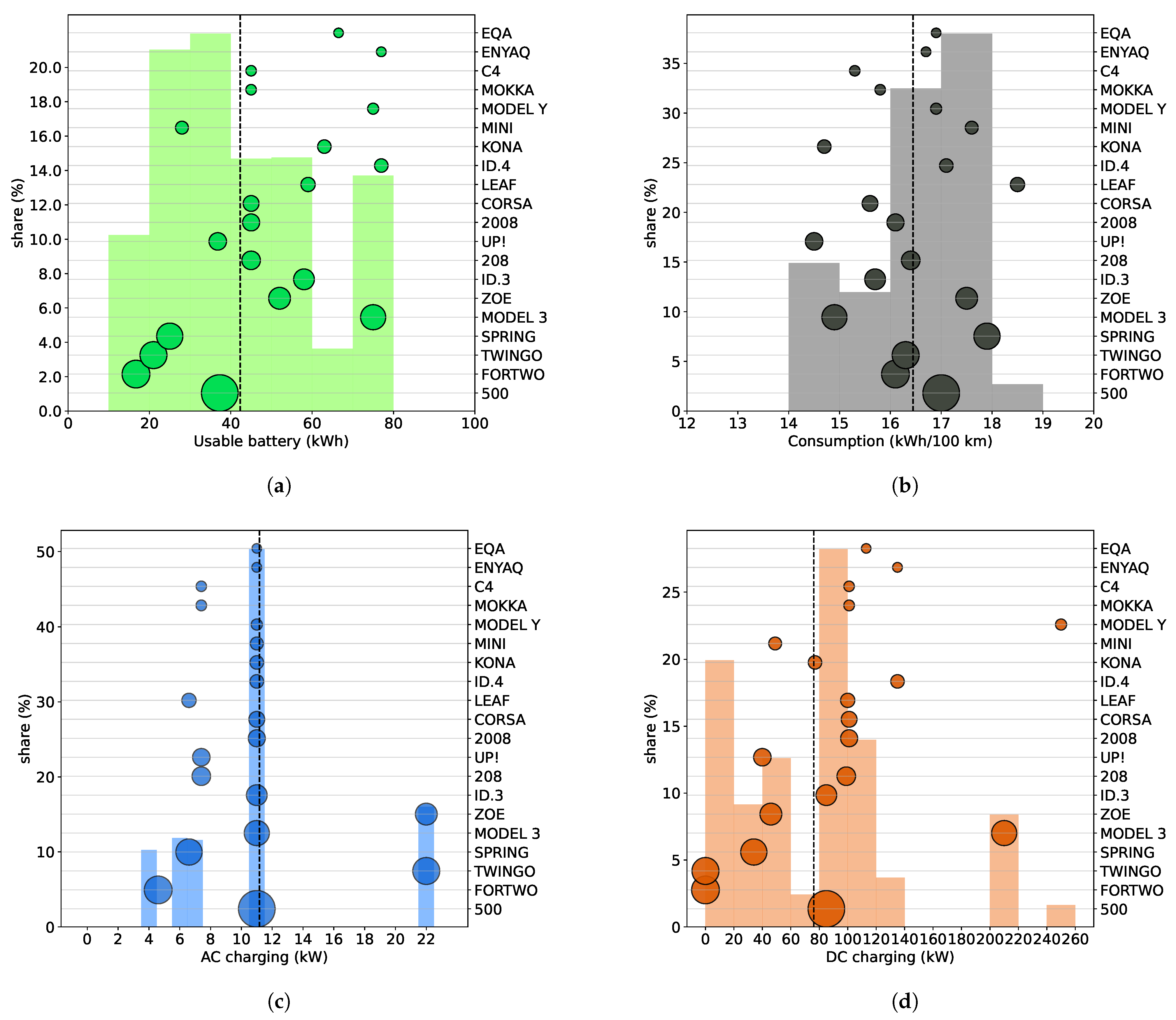
data frame contains information about the EVs population derived from the distribution of the models’ share summarized in
Figure 3. Along with the EV model,
reports the corresponding value of battery capacity
(in kWh), the ID number associated to each model, and the maximum charging capability in AC (
) and DC (
) modes (both in kW). To each
is assigned a
value (in percent). The
is obtained according to the procedures described in
Section 2.3.
The last columns of
report the arrival time, departure time, and parking duration of the
i-th EV (expressed in hours). These values are obtained considering the analysis carried out in
Section 2.2 and according to the selected parking lot scenario
S. The values of
,
, and the relative
are computed starting from their distribution so as to obtain a population of
N samples whose probabilistic trend respects that of the selected scenario.
For each
, the charging time
is defined as the period between the initial time of charging
, that is the instant in which
is plugged in, and the final time of charging
:
The end-charging time may depend on two conditions:
The vehicle is plugged and the SOC reaches the maximum value. Hence, the charging stops and ;
The vehicle is unplugged because the users leaves the parking lot even if the charging is incomplete. Hence, .
It is assumed that the instant of arrival in the parking lot coincides with the beginning of the charging, therefore:
On the other hand, the final charging instant could coincide or not with the departure time of the vehicle from the parking lot. This condition is governed by the following equation set:
The second step of the proposed method is to define, for each
i-th EV, an array that contains the value of
for each discretized instant
of the day. In this work, a discretization time resolution
is considered. Thus, the
-array for a 1-day calculation consists of
elements. Considering the whole population of
N EVs it is possible to define the
matrix
whose element
represents the power required by the
i-th EV (row-index) at the
-th minute of the day (column-index). Similarly, it is possible to define the matrix describing the vehicle presence in the parking lot, called
, and the matrix of the
evolution, called
. The elements of
are of Boolean kind; specifically
if the
i-th vehicle is parked at instant
, otherwise
. The element
represents the state of charge of
at the instant
. It is clear that
and is initialized through the value of the
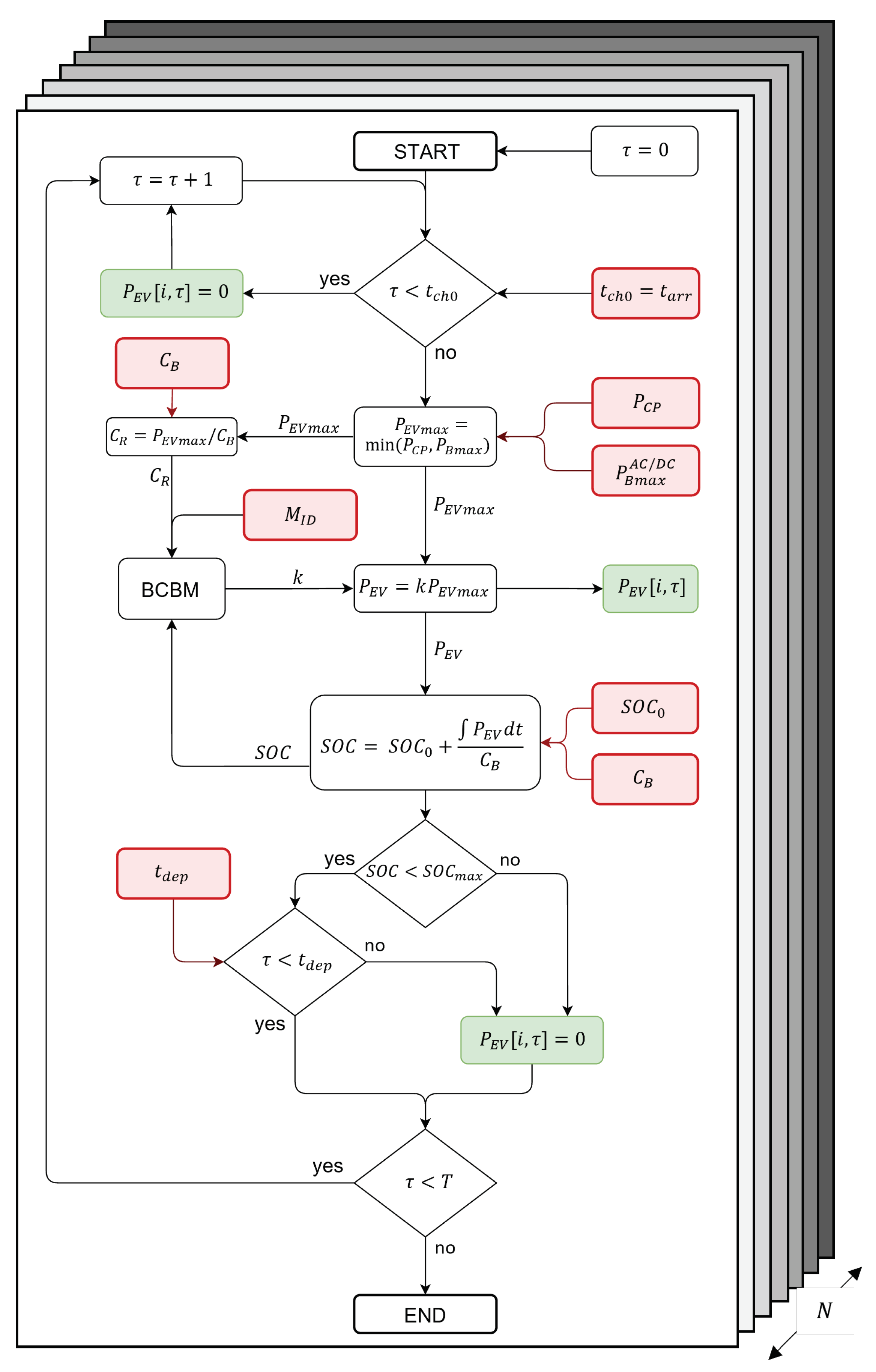
data frame. The following forecasting algorithm logic is shown in
Figure 11.
Considering an
N-users population the algorithm runs in parallel for each EV (
-row) in order to fill all the elements of the
matrix. The algorithm starts the calculation by referring at the time
(beginning of the day, i.e., 00:00). For each
the algorithm is initialized through the
i-row of the
data frame, whose data are represented by the red box in the flow chart of
Figure 11. The resulted powers are highlighted through the green boxes.
As long as , the vehicle is not present and , the output is zero. As soon as the vehicle arrives in the parking lot, switches to one and keeps this value as long as the vehicle is parked. is initialized to and the algorithm starts calculating the charging power.
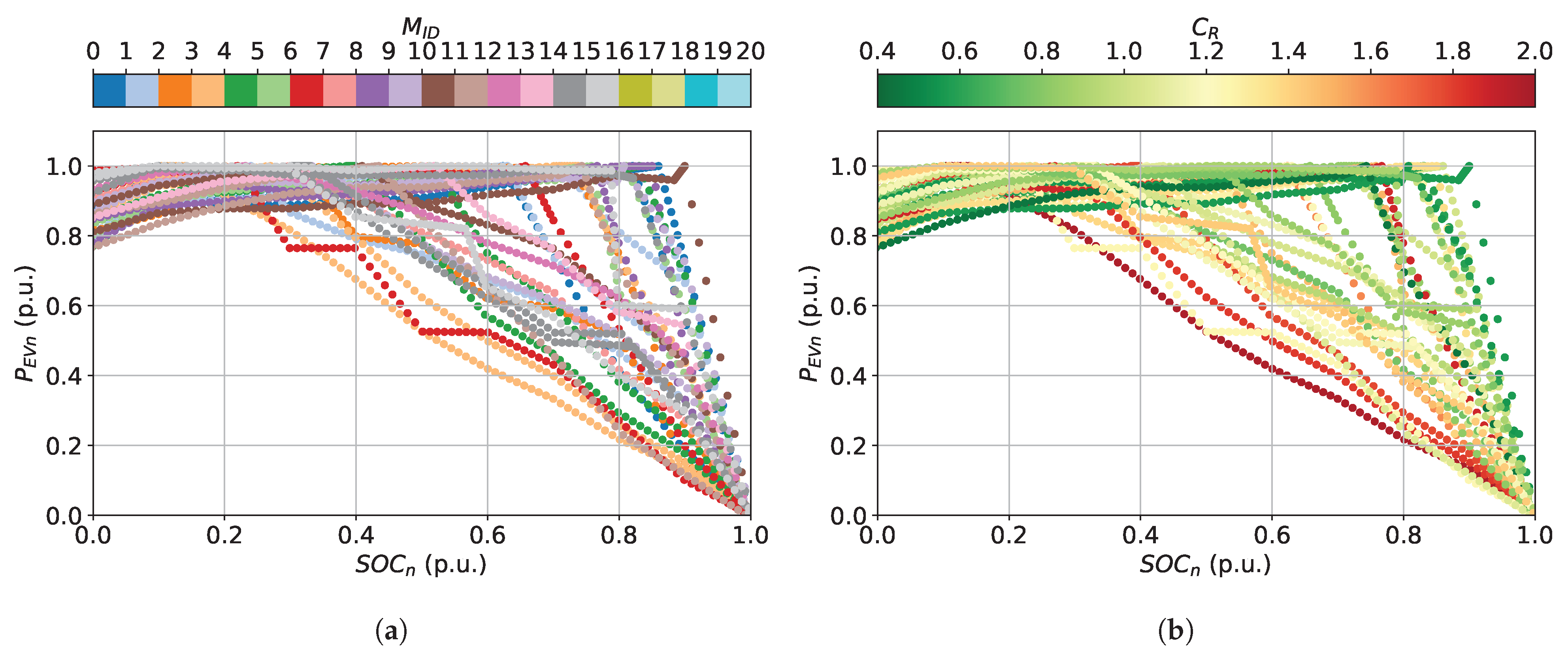
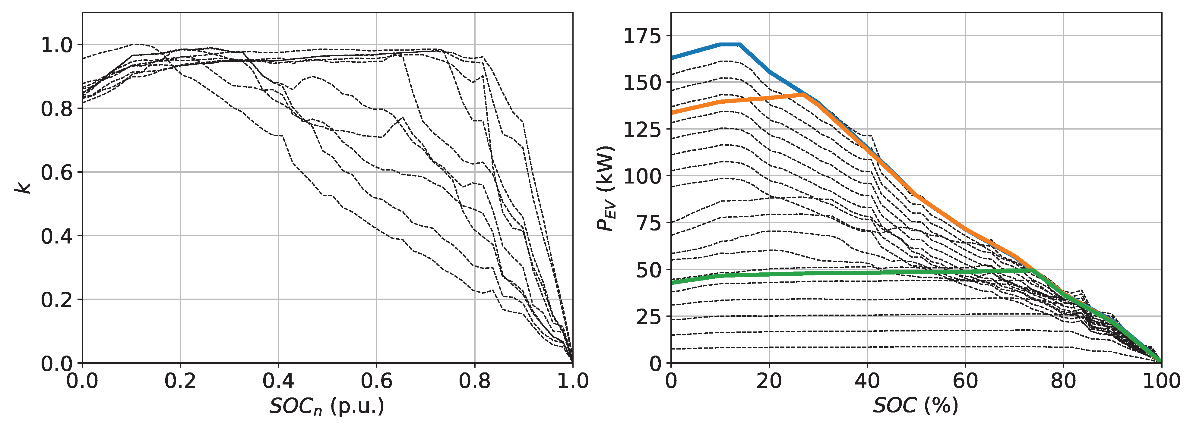
After that, the initial value of the power is multiplied by a scale factor
k according to
Section 2.4. The
k parameter is the output of the BCBM and sets the power absorption of
according to its
,
, and relative C-rate. The algorithm updates the SOC in each iteration by calculating the battery’s energy through charging power integration. Accordingly, the element
of
at the instant
is obtained by Equation (
10):
where
and the term
represent the cumulative energy (kWh) from the start of charging to the
-instant. The charging process can stop (
) if condition of Equation (
9a) or (
9b) occurs. Finally, the algorithm stops computing at
(end of the day, i.e., 24:00).
Once the
matrix is calculated for each
it is possible to obtain the total power profile of the charging hub containing the contribution of each
:
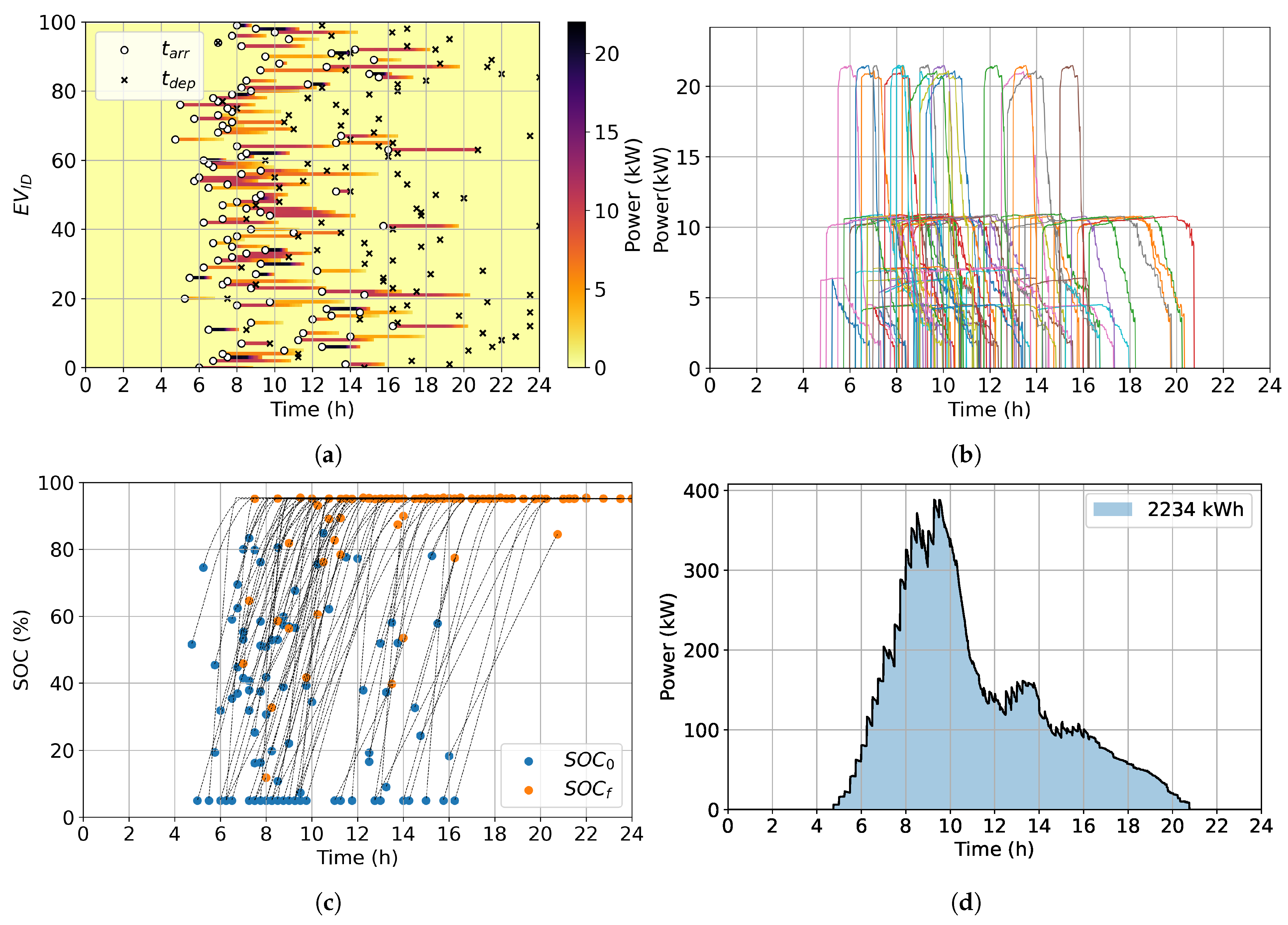
As an example,
Figure 12 shows the results of the proposed algorithm considering a 100-EV population and a charging hub having AC CPs of
. The charging hub is located in a working place parking lot. The scatter plot in
Figure 12a shows the arrival and departure time randomly generated from their scenario pattern (
Figure 4c).
Figure 12a also shows
as a heat map. The heat map represents the power level that the EVs require from the CPs during the charge. The color variations depend on the modulation due to the BCBM.
Figure 12b shows the charging power profile of each EV belonging to the N-users population. It is evident how the power profile varies during charging depending on the vehicle model, C-rate, and the evolution of the SOC. Although
, only a portion of EVs manage to use all of CP power (mainly the Renault ZOE). Most vehicles receive a maximum power output of
or less.
Figure 12c shows the value of the SOC at the arrival time and at the departure time. The black dashed line depicts the evolution of the state of charge as a function of time,
. Finally,
Figure 12d shows the total power required by the charging hub,
obtained from Equation (
11). The figure shows a peak of about
at the peak of EV arrivals. Through the algorithm, it is also possible to calculate the total energy required daily by the CH, which is about
and is represented by the blue area in
Figure 12d.
4. Results on Different Scenarios
The following section analyzes and discusses the results obtained from the proposed forecasting algorithm. Comparisons are conducted considering the possible variations of the algorithm setting parameters. Specifically, the effects on the power profile of the number of daily users, the charging stations’ power rating, and the parking scenario are analyzed in detail.
Table 5 shows the settings of the algorithm input parameters selected to compare the results.
The values of
is set to match all the charging level categories reported in
Table 1, from slow AC-charging to ultra-fast DC-charging. The
is set according to the related power level. Four charging hub daily users numbers from 10 to 200 EV/day are selected in order to evaluate a possible temporal increase in EV penetration or a different size of the parking area.
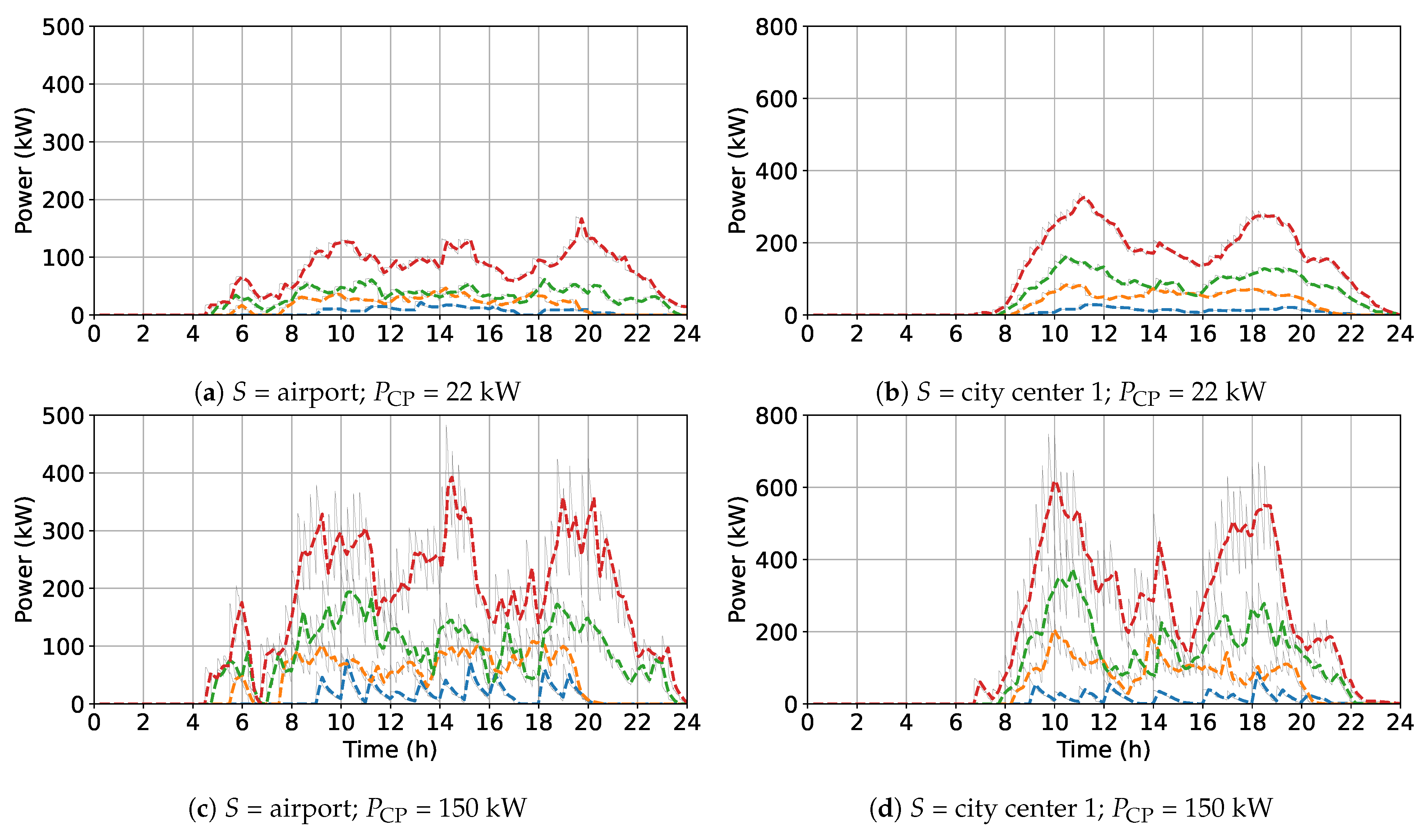
Figure 13 and
Figure 14 show some preliminary results. The figures represent the daily power profiles (24-h time window) for 4 different scenarios as the charging points’ power and the number of daily users change. The gray lines depict
(with a 1-min resolution). The dashed colored lines depict the
moving average whose color is a function of the
N-setting. The
selected for
Figure 13 and
Figure 14 are
(that is the upper limit of the most common AC-charging level) and
(that is the upper limit of the most common DC category).
It is possible to see how the profiles are more pulsed the higher is the CP power. This phenomenon is mainly due to the arrival of new users who can each potentially increase consumption by at the instant of connection. The CH peak power is also naturally affected by and N. In addition, the results show that the peak power and, in general, the evolution of the whole profile strongly depend on the scenario S under consideration.
For the same number of daily users, the scenario with a more concentrated distribution of arrivals and longer parking time exhibits a contemporaneity of charging events. More users connected for a longer time implies a higher demand for instantaneous power and total energy. This phenomenon can be observed by comparing
Figure 13a,c with
Figure 13b,d. As described in
Section 2.2, the “working” scenario has a more concentrated distribution of arrivals (peaking around 8 a.m.) and a longer average parking time. This affects the simultaneity of charging events compared to the “mall” scenario, which instead has a more distributed probability of arrivals and a shorter vehicle dwell time. As a result,
Figure 13b,d shows higher peaks (about twice as high) than
Figure 13a,c. This difference is more pronounced the higher the number of daily CH users
N. Similar considerations can be done in
Figure 14 where another parking scenario in analyzed.
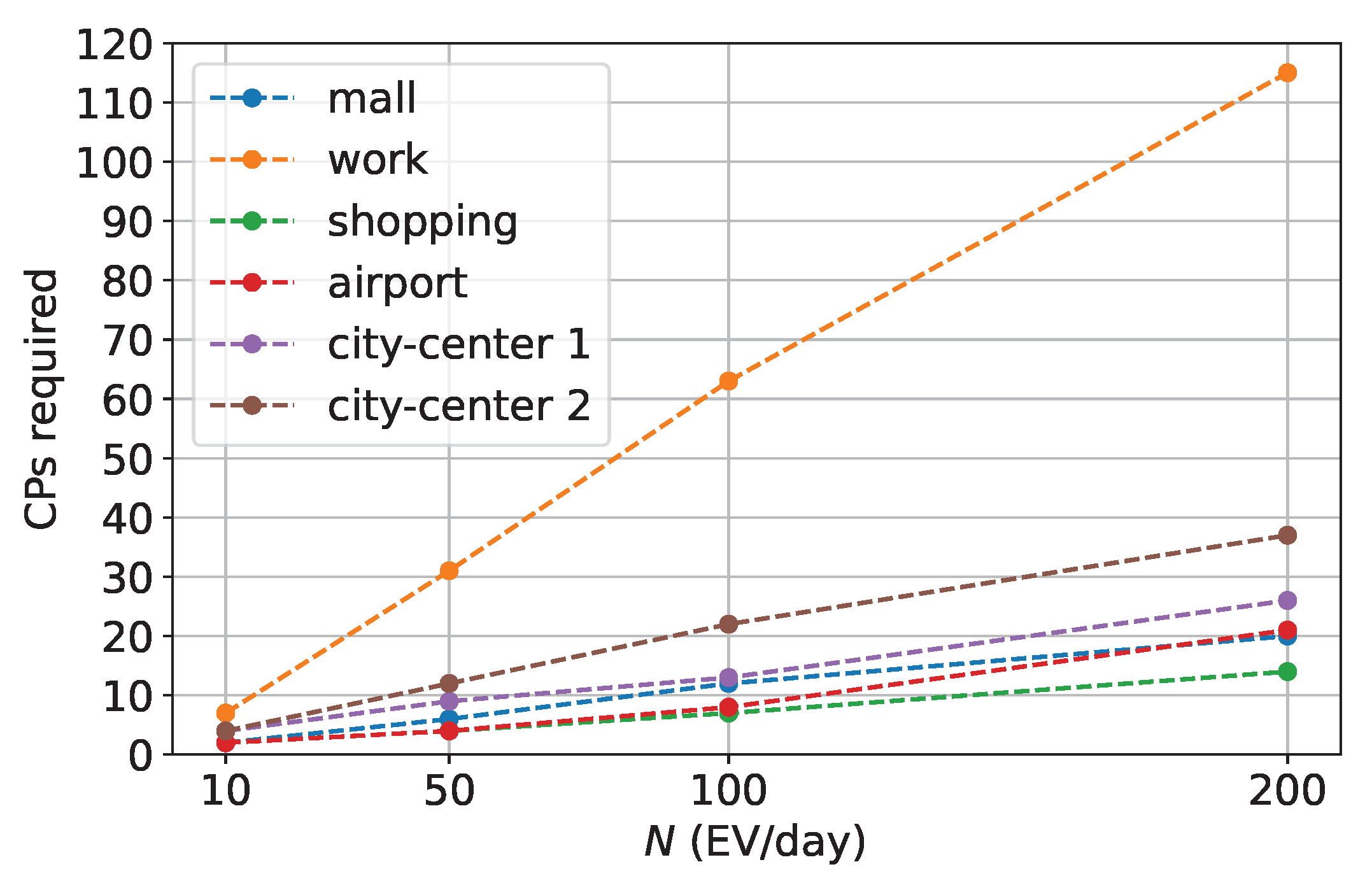
Based on the parking lot scenario, it is possible to analyze the simultaneity of the charging events through
Figure 15. The proposed algorithm allows us to evaluate the instant and the duration of the users’ connection time. Then, it is possible to calculate the number of users simultaneously connected to the charging hub. From a complementary point of view,
Figure 15 shows the number of CPs that the CH should have to satisfy the entire fleet of
N users per day.
It is therefore possible to state that the parking scenario influences the sizing of the CH in terms of peak power required, the number of CPs to be installed to satisfy the entire fleet of N users (simultaneity of charging events), and finally the average energy deliverable to vehicles. The following sections quantitatively analyze the results by comparing the scenarios in these respects.
4.1. Analysis on the Charging Hub Peak Power
Although the simulations are initialized with models that follow a defined pattern, the individual elements of the initialization data frame (
,
Table 4) own a random nature. Therefore, it may occur that the algorithm generates slightly different power profiles despite being set with the same input values. To provide adequate statistical significance to the results shown in the following, multiple simulations are performed for each input data setting. The final output results from the averaging of the values of each simulation run.
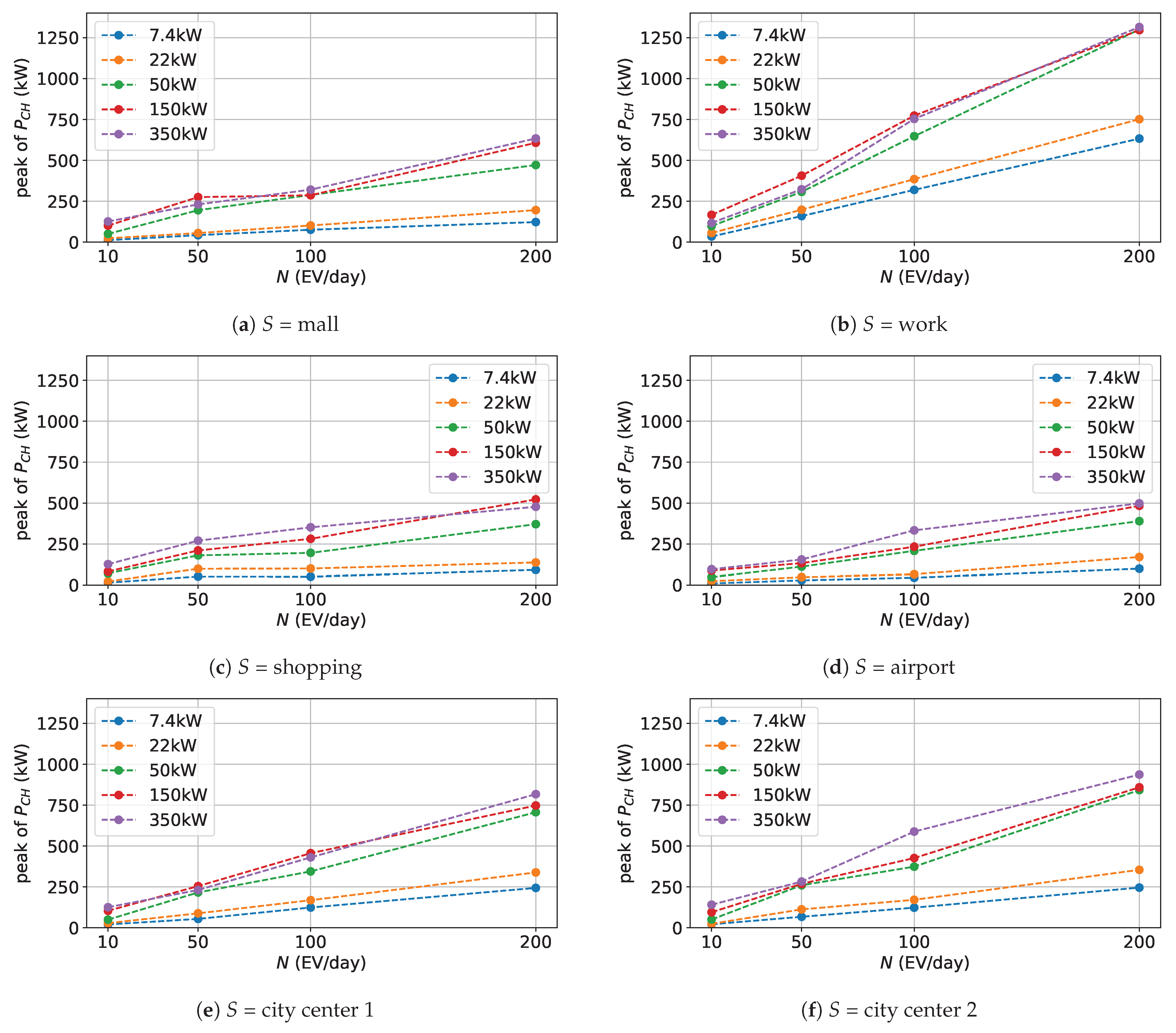
Assuming that the CH is sized to have the optimal number of CPs to satisfy all users (as in
Figure 15),
Figure 16 shows the peak power absorbed by the CH (peak of
) from the grid as a function of
N for the scenarios under study. Different colors in
Figure 16 depict different values of the CP power
. The most common sub-categories of
Table 1 are selected for comparison.
The figure shows a quite linear proportionality between
N and the peak value of the CH power profile. Specifically, the analysis conducted in this subsection confirms the dependence of
on the number of EVs simultaneously connected (
Figure 15).
On the other hand, results show that there is no direct proportionality between the peak power and the power rating available at the charging points. For example, let refer to the case
in
Figure 16e which considers the “city center 1” scenario. The greatest increase in peak power occurs at the transition from
to
. Thereafter, tripling the CP power does not imply a noticeable increase in peak power. Moreover, in almost all the scenarios analyzed, from Fast to Ultra-fast CPs, the peak power variation is very slight in comparison to the
variation. This is mainly due to the few numbers of EVs having a charging capability above
among the total population (as reported in
Figure 3). This means that currently, for the same number of daily users and available CPs, the contracted power of a CH that has
CPs could potentially be similar to a CH that has
CPs.
4.2. Analysis on the EV Fleet Charged Energy
This subsection compares the total energy provided to the EVs by the CH under different input settings. The total daily energy that CH supplies to the EVs, named , depends on the charging power and charging time . However, the real values of used power is limited by the maximum power that the vehicle’s battery and onboard converter can accept. Therefore, there could be a sort of threshold value of beyond which, further increase in the nominal power of the CPs would not result in an increases in the total energy delivered to the EV population batteries. The parking scenario influences users’ parking time and thus, for the same power output, itaffects the total daily energy delivered to EVs. It may be possible that scenarios with lower require higher to meet the energy needs of EVs.
Through the proposed method, it is possible to address these issues and evaluate the CH’s ability to meet vehicle energy demand under different parking scenarios. The comparison proposed in this section focuses on the daily average energy supplied to the EV population (kWh/users) and their average state of charge at the departure time (
). Simulations run considering
for each
S. The value of
varies in the range shown in
Table 5.
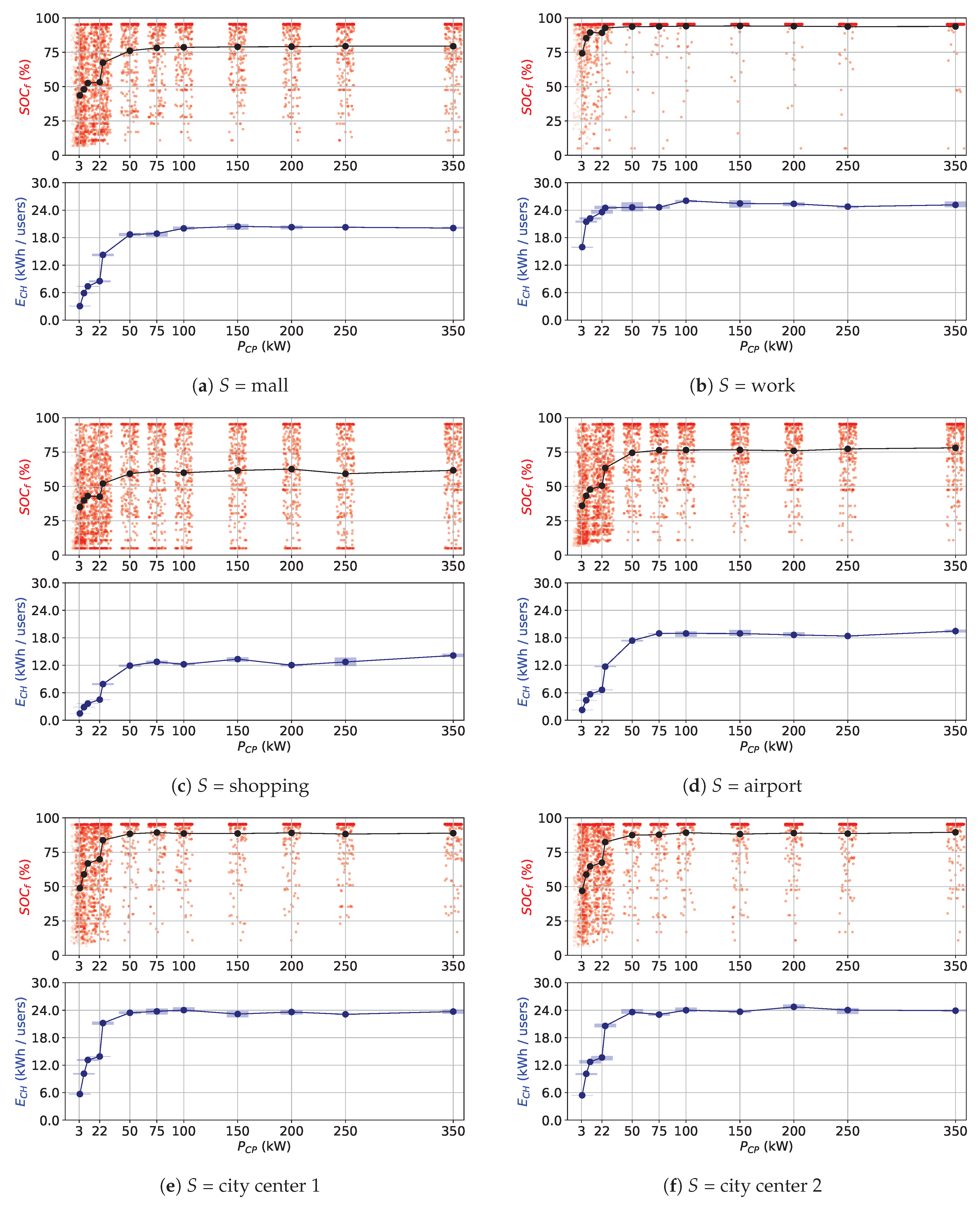
Figure 17 shows the values of EVs’ SOC at the departure time, which are depicted by the red dots (top-frame of the sub-figures). The black line with round markers represents the average value of
. On the bottom frame of the sub-figures, the blue markers depict the average energy supplied per EV (kWh/user).
The figures point out clear differences among scenarios. In the working place parking scenario (
Figure 17b), results show that high power levels do not imply significant additional increase in
and
. This is due to the longer
, where EVs stay parked long enough to ensure adequate
even at low
. The figure shows a slight increase in
at the transition between AC and DC charger (
to
) due to the bypass of the onboard charger that enables charging at higher powers. Higher values of
seem to produce no improvement in delivered energy
, that remains at
, and in the average
, whose value remains close to
).
Considering other scenarios which have a lower
, it is evident how switching from AC
to DC
CPs results in a significant increase in the delivered energy and the associated average
. The
Figure 17a,d–f show that for a small increase of
in
, the energy delivered per vehicle doubles, and
exhibits a radical increase. For example,
Figure 17e,f show that
increases from 13 to 20 kWh/users and the average SOC from 66% to 82% in the case of city-center scenarios. Thereafter, performance increases as
increases and then saturates at
between
and
. In the case of shopping scenario (
Figure 17c) where the parking time is extremely short, even if
increases the energy delivered to EVs cannot reach more than 14
and the increase in
is negligible.
It is important to emphasize that the results obtained are valid under the assumption expressed by Equation (
9b), or, in other words, that the charging time is considered equal to the parking time. Clearly, this assumption loses its validity in the event that the user extends the parking time to reach an higher SOC at departure. However, it is worth reiterating that the analysis performed aims precisely to investigate the capability of the CH to provide adequate energy to users without altering their behavior (i.e., usual parking time).
Results show that, in general, Slow DC charging points enable better performance in terms of and compared to AC chargers having similar power ratings. Considering the working scenario, the AC medium-level charging is sufficient to ensure adequate to the whole EV fleet. For all other scenarios analyzed, a good trade-off between , values and the CP power output is . Fast and Ultra-fast charging point seems not to bring an improvement in the performance markers under study.
Finally,
Table 6 shows the summary of the analysis carried out in this section. The table compares the scenarios considering
N = 100 users per day. For each scenario, the table reports the number of CPs needed to ensure connection to each EV in the fleet, the CP power rating suggested to avoid over-sizing and ensure an adequate
, the peak value of the CH power, and the average energy supplied per user.
5. Conclusions
The work has aimed at providing a method for forecasting the power demand related to a charging hub for EVs in different parking scenarios.
The method tried to take into account all the main factors that may influence the power demand. The preliminary analyses on the charging stations and EV models currently available revealed a significant heterogeneity in the values of power levels of the charging stations and in the battery capacities and accepted power levels for the recharge among the different EV models. At the same time, the absorbed power profile of a charging hub is influenced by other factors such as the arrival and departure time, and parking duration of EV users. These parameters change strongly according to different parking scenarios (e.g. malls, airports, urban car parks, etc.) Finally, for each charging process, the EV energy demand also depends on the state of charge at arrival at the charging hub.
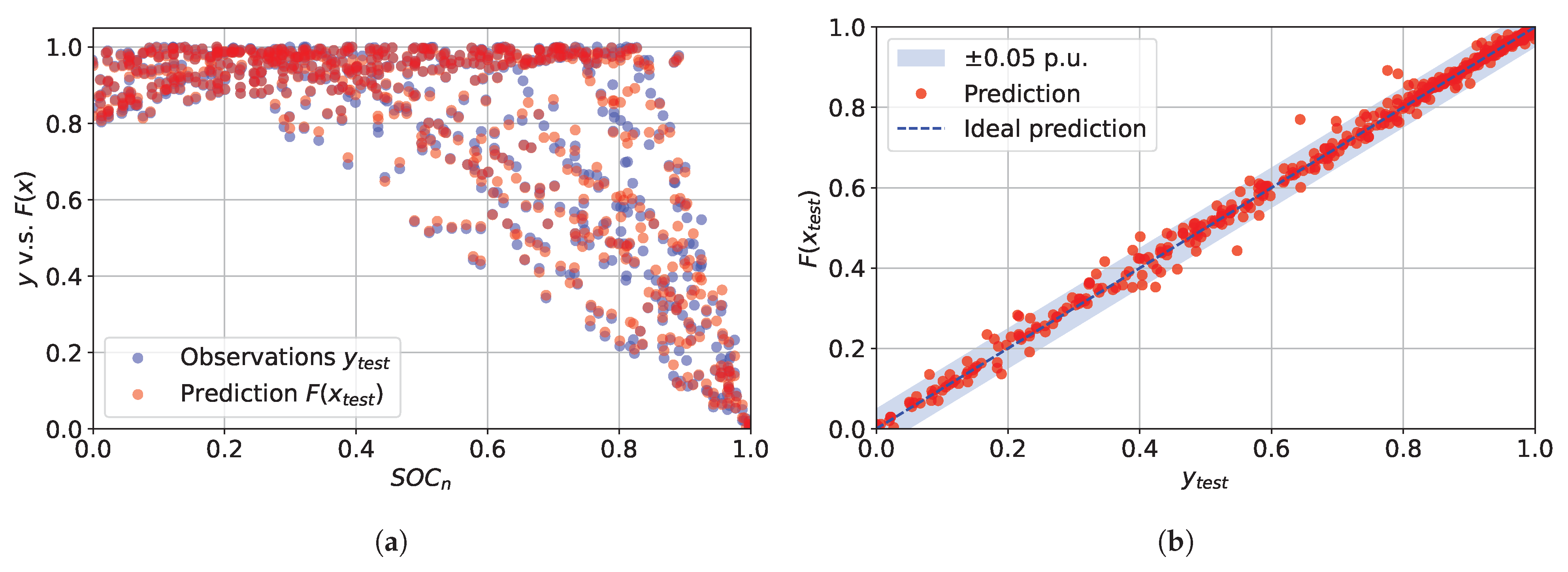
Given the complexity, numerousness, and aleatory nature of the various factors considered, a probabilistic approach was used to generate a model of the vehicle population and user behavior under different parking scenarios in terms of arrival, departure, and parking duration times. The analysis of an extremely large sample of trips combined with the statistical distribution of the battery capacities of the electric vehicles on the road and the charging needs as a function of distance traveled has made possible to obtain a distribution of the state of charge of the EVs at their arrival at the charging hub. A supervised machine-learning model has been adopted to reproduce the behaviour of the battery during the charge as a function of the charging rate, the considered EV model and the evolution of the SOC during the charge. The model allowed to obtain the absorbed power profile associated to each charging event. The model has been trained and tested by using the power curves of different EV models, under different charging rates. The derived model has fit the test data with an RMSE = 0.017 and R2 = 0.996.
The resulting models from each analysis have been integrated in the final algorithm capable of forecasting the absorbed power for the charging of an electric vehicle fleet in the time domain.
The results section compares the algorithm outputs considering different combinations of the input data, namely: the parking scenario, the number of daily EV users, and the characteristics of the charging infrastructure (i.e., power rating and category of the CPs). The proposed algorithm proved its high effectiveness in assessing all major aspects essential for planning and sizing charging hubs in different installation scenarios. As shown in the results section, the algorithm allowed the evaluation of the optimal number of CPs to be installed to satisfy the demand of a certain EV fleet, the peak power required by the CH from the grid and the total energy daily delivered to each vehicle together with their final state of charge.
Analysis of the results showed marked differences between the power profiles of the scenarios analyzed. CH located in a working place scenario requires more CPs to satisfy the same number of users per day compared to other urban scenarios. On the other hand, AC charging points are sufficient to meet the energy demand of the entire fleet. In fact, the results proven that DC chargers do not introduce significant improvements. The other urban scenarios, which have a lower probability of simultaneous user connection, require fewer CPs for the same number of daily charging events. However, due to the shorter parking times, fast DC CPs are needed to ensure an adequate energy supply. In this case, rated powers between and are sufficient to meet fleet energy demand. In general, considering the characteristics of the current EV population and the typical parking times of urban scenarios, the proposed method showed that the use of ultra-fast (i.e., ) charging points produces no increase in average energy delivered. Similar considerations can be made regarding the SOC level of vehicles at the end of charging and the total peak power.
Future works can consider new parking scenarios like residential, home charging, and highway parking. Moreover, also the residential overnight charging can be considered for the computation of the pre-connection SOC. Finally, starting from the proposed EV load forecasting, future research can investigate sizing methods to optimize the design and management of PV and battery systems integrated with the charging hub.


 ,
, 


