Abstract
Optimization-based design tools for energy systems often require a large set of parameter assumptions, e.g., about technology efficiencies and costs or the temporal availability of variable renewable energies. Understanding the influence of all these parameters on the computed energy system design via direct sensitivity analysis is not easy for human decision-makers, since they may become overloaded by the multitude of possible results. We thus propose transferring an approach from explaining complex neural networks, so-called locally interpretable model-agnostic explanations (LIME), to this related problem. Specifically, we use variations of a small number of interpretable, high-level parameter features and sparse linear regression to obtain the most important local explanations for a selected design quantity. For a small bottom-up optimization model of a grid-connected building with photovoltaics, we derive intuitive explanations for the optimal battery capacity in terms of different cloud characteristics. For a larger application, namely a national model of the German energy transition until 2050, we relate path dependencies of the electrification of the heating and transport sector to the correlation measures between renewables and thermal loads. Compared to direct sensitivity analysis, the derived explanations are more compact and robust and thus more interpretable for human decision-makers.
1. Introduction
Energy system design (ESD) tools allow domain experts to build and optimize energy system models concerning system costs or CO emissions. Various modeling frameworks exist, such as TIMES [1] and OSeMOSYS [2], typically based on linear optimization. Ready-to-use implementations including model equations and data are available for countries such as the United States [3], United Kingdom [4], or Germany [5]. All such models are based on a multitude of parameter data. Required data include time series, technical and economic parameters, and legal and physical limitations. For example, for modeling wind power, historic weather time series for the wind speeds, the currently installed capacity of wind power plants per model region, the specific costs for new installations, and the maximum possible capacity allowed by regulation are required. When no data are available, assumptions have to be made. The computed ESDs are highly dependent on these data and assumptions. The dependence can even be counter-intuitive [6]. A robust interpretation of these optimization models’ outcomes thus requires detailed knowledge of the models and their inputs.
The people who decide on the real-world implementation of computed ESD proposals are typically non-experts in the field of energy system modeling. Such decision-makers can be CEOs responsible for their companies’ CO footprint, politicians responsible for shaping energy regulation, or citizens responsible for their own homes and electing the politicians that fit their needs. All these actors take personal risks when deciding about ESDs, with respect to either financial or electoral consequences. In order to promote informed decision-making of these non-experts—or indeed to promote any decision-making at all—intuitive explanations of the computed ESD proposals are essential to build the required trust into the model outcomes [7]. In addition, experts could greatly benefit from good, intuitive explanations, e.g., to verify their modeling assumptions and result interpretations.
A tool often used by domain experts to explain ESD tools’ results is sensitivity analysis, which creates explanations based on how a system reacts to individual parameter changes. The term sensitivity analysis is used for methods that vary the input of a model and observe the change in outputs. Approaches differ in how they change the inputs; e.g., changes can be infinitesimal or finite, and variations can be deterministic or probabilistic. For a general overview of sensitivity methods, see [8,9]. For sensitivity analysis applied in the context of ESD, see [10,11,12]. For models formulated as linear programs, differential sensitivities are easily accessible as a byproduct of the dual problem solution [13]. They are then called “marginals” and can be used to answer questions such as “What is the value of an additional unit of capacity of a power plant?” or “What is the effect on the battery capacity if the electricity demand at 8:15 a.m. would be 1 unit lower?”.
Model sensitivities for high-dimensional input parameters, such as demand or renewable time series, are often not helpful since small changes in parameter values for individual time steps often have only a minor impact on the optimal system design. Changes for multiple time steps, however, can have a significant impact. For example, suppose the renewable energy potential is increased for a single time step. In that case, it is unlikely that the cost-optimal storage capacity changes since additional storage capacities are expensive when used only once. If the renewable increase covers several well-distributed time steps, storage capacity can be reused and becomes more attractive. This argumentation shows that changes in high-dimensional parameters such as time series are relevant for decision-makers, even when sensitivity analysis of individual values is not informative.
Machine learning methods also often have high-dimensional inputs and the need to explain their decisions [14]. The input data for many classification methods are high-dimensional data structures such as images or texts. Since a change in an individual input dimension, i.e., a pixel or a letter, should not change the class prediction, and sensitivity analysis based on these variations is not very informative. Moreover, models such as neural networks and random forests include large numbers of complex operations that are often not transparent to the user. Their information processing is thus often conceived as a black box. A popular explainable AI method to overcome these limitations is “locally interpretable model-agnostic explanations” (LIME) [15]. LIME, designed for application to classification problems, addresses the shortcoming of traditional sensitivity analysis regarding high input dimensions by introducing an interpretable abstraction layer for the input features. It then aims to find the interpretable features whose variations are most relevant for changing the predicted class label. This feature is then considered most relevant for a given class decision.
In this paper, we propose to transfer the LIME idea from the machine learning domain to the ESD community given the parallels between the two described problem settings. While explainable AI methods have been used in energy and power systems before, explaining machine learning-based models employed in power grids, the energy sector, or energy management in buildings, see e.g., [16,17,18] and the review [19], we use explainable AI methods here for energy system design, where not statistical learning methods but an optimization problem is at the core. Specifically, the key contributions of this paper are as follows:
- We employ the LIME idea to create explanations for the outputs of ESD tools that are based on bottom-up optimization models. To this end, we establish the parallels between the two problem settings and the possible solution approaches.
- We demonstrate how to create interpretable abstraction layers for ESD settings.
- We showcase exemplary explanation results for a building and a nationwide ESD model, improving on the traditional sensitivity analysis.
By making ESD better understandable to non-expert decision-makers, we hope that the work supports informed decision-making in the transition towards low-carbon energy systems.
The remainder of the paper is structured as follows: An exemplary ESD model of a building with a renewable energy supply is presented in Section 2. It serves as a running example throughout this work. We then explain the concept of LIME and show how the methodology can be transferred from the machine learning domain to ESD models in Section 3. Explanations for the optimal design of the exemplary energy system are derived and discussed in Section 4. Explanations of a more complex model, i.e., a model of the German energy system, are presented in Section 5. A conclusion is given in Section 6.
2. An Exemplary Building Energy System
This paper uses a building energy system as a running example. Its structure is shown in Figure 1. The building is characterized by an electric and a thermal demand. Electric energy is locally generated by a photovoltaic (PV) plant or can be bought from the external electricity grid. Electricity can be stored in a battery for later use and converted into heat using a heat pump. Heat can be stored in heat storage, such as a hot water tank.
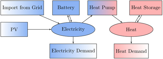
Figure 1.
Schematic overview of exemplary energy system model of a building with photovoltaic (PV) power plant. Energy commodities are displayed as ellipses and energy conversion processes as rectangles. Arrows of a conversion process denote which energy commodities can be transformed into each other, while colors encode different types of energy. Conversion processes without input or output represent energy demands or energy imports into the model domain.
The energy system is modeled using a bottom-up approach based on linear programming [20], extending the model of [7] by a heat sector. The model’s objective is to minimize the total system costs, including investment and operational contributions. Optimization variables are the scheduling decisions of all components, e.g., when to charge or discharge the battery. Furthermore, the system’s design is optimized by model-endogenously choosing cost-optimal capacities for the battery and heat storage. In contrast to [7], the PV power plant capacity is assumed to be known. The model adheres to a set of constraints. These include the power balances for electricity and heat at every time step. Other conditions describe the storage level’s dependency on charging and discharging decisions. Three sets of inequalities limit the available PV energy per time step to an externally given, weather-dependent time series, ensure feasible storage levels, and constrain the heat pump’s power output by capacity. The detailed mathematical equations are given in Appendix A.
3. Proposed Explanation Methodology
In this section, we present our methodology to derive explanations for ESD models that go beyond the scope of traditional sensitivity analyses. As our approach is based on the LIME [15] method from the explainable machine learning domain, we first describe LIME in its original context and then introduce our proposed methodology in parallel.
3.1. LIME for Machine Learning
LIME introduces an interpretable abstraction layer for the input dimensions of the machine learning task and combines it with a modified sensitivity analysis. As the name “local interpretable model-agnostic explanation” suggests, LIME creates explanations for non-experts for any classifier given a specific point of interest (POI) , where is the original input space of the classification problem and L is the number of class labels f can predict. The created explanations are local, i.e., only valid for variations close to the POI. To this end, an interpretable feature space is created for the original, high-dimensional input space of the classification problem with . The vector is a binary vector encoding the presence or absence of interpretable features related to the POI . First, I variations in the interpretable feature set are made around . Second, a function maps the interpretable variations back to the input space, i.e., . Each variation is then weighted by based on its similarity to . Finally, LIME determines the most important interpretable features, i.e., the explanation, for a given class label by solving the regularized least-squared regression
where the model is a model in the class of all linear models and is a complexity measurement of , for example, the number of non-zero weights of g. Interpretable features with non-zero weighting are then deemed explanations for the classifier’s local behavior around the POI . By choosing appropriately, the complexity of the explanation can be limited as desired.
A visualization of the concept of LIME applied to image classification is found in Figure 2a, where an interpretable explanation for the classifier f’s prediction of the “dog” class is created by LIME. The original input space contains vectors with the color values of the individual pixels of an image. Clusters of pixels, the so-called super-pixels, are used to define the interpretable feature space . Each interpretable feature encodes the presence or absence of a super-pixel. Variations around the interpretable representation of the image are made. Those variations are mapped back to the input space by replacing all pixels belonging to a non-selected super-pixel with a neutral color, i.e., a 50% grey value. The resulting inputs are classified by f, and a linear model g is fitted to the resulting “dog” class probabilities by solving the problem defined in Equation (1). The magnitudes of the weights in g represent the impacts of the super-pixels on f and can thus be used to explain f locally. The complete explanation is a list of super-pixels in decreasing order based on their absolute impact on the class label. Shown in green is the super-pixel with the highest weight for predicting the class “dog”; shown in red is the super-pixel with the highest weight for not predicting the class “dog”.
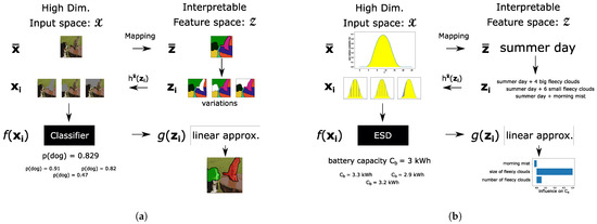
Figure 2.
(a): The LIME method: For an image classifier where individual pixels of an input image have no explanatory power, an abstraction layer with interpretable features (here super-pixels) is created. Variations around the interpretable representation of the input image are made and mapped back to the input space via , i.e., by replacing each pixel belonging to a super-pixel with a single neutral color. The classifier f is applied to the modified inputs. LIME fits a linear model to the classifier’s outputs and uses g to explain the behavior of g locally around . (b): Proposed Method: For a high-dimensional input , e.g., a radiation time series, interpretable features that could be relevant for explanation are identified. Variations around are made and mapped back to the input space by . The ESD model f is optimized for each input variation . A linear model is fitted to the output of the ESD optimization, e.g., the cost-optimal battery capacity . The weights of the linear model g represent the relevance of the interpretable features for the output of the ESD model f locally around .
3.2. Proposed Method for Explaining ESD Models
We now want to explain to non-experts an output value from the cost-optimal solution of an ESD model. To this end, we propose a method based on the LIME concept, where instead of a class probability given by the classifier, we explain an output value of a cost-optimizing ESD model. The POI is a vector in the ESD model’s input space . We then identify interpretable features that may or may not be part of the original model parameters but are assumed to be potentially relevant for an explanation. Since we are interested in quantitative explanations and not only qualitative ones, instead of the binary encoding used by LIME for the interpretable features space, we define . Similar to LIME, variations in the interpretable features are mapped to the model’s inputs via a mapping between the interpretable features space and the input space . The ESD model is optimized for each variation. A linear model is fitted to the results of the ESD model runs by minimizing the objective in Equation (1). As the complexity measure , we chose the number of non-zero weights of g. The linear model g is finally used as an interpretable explanation for the ESD model: a weight in g corresponding to an interpretable feature represents that feature’s influence on the ESD model’s output.
A visual representation of the methodology proposed for the explanation if ESD is shown in Figure 2b. The illustration is based on our exemplary building energy system from Section 2. An interpretable explanation for the cost-optimal battery capacity designed by the ESD model is created for a given set of input parameters, the POI . In the presented case, the POI is a summer day’s solar radiation time series. An interpretable feature space is then created. Interpretable features considered potentially relevant for an explanation are the specific battery investment cost, the number and shape of “fleecy clouds” occurring during the day, and the existence of “morning mist”. Interpretable variations around the POI are made, and the mapping maps the interpretable variations to the models’ input space , resulting, e.g., in variations in the solar radiation time series. The ESD model is then optimized for each variation. A linear model g is fitted to approximate the cost-optimal battery capacity of the ESD model’s results. The weights of the resulting linear model g are taken as an interpretable explanation for the ESD model. A weight in g corresponding to an interpretable feature represents that feature’s influence on the ESD model’s output. In the given example, the most relevant interpretable feature for the ESD model’s cost-optimal battery capacity is the size/duration of the “fleecy clouds”.
4. Experimental Demonstration: The Exemplary Building Energy System
In this section, we apply our proposed method to create an explanation of the cost-optimal battery capacity for our exemplary building energy system introduced in Section 2. To this end, we first define a set of interpretable features that can impact the cost-optimal battery capacity. They consist of cloud characteristics, the PV surplus with respect to the load, and the specific battery investment cost. These features are described in Section 4.1. Section 4.2 describes details of the first implementation of our methodology to the exemplary building energy system. Section 4.3 shows results for our proposed method on a simplified version of the same exemplary energy system model, which includes only the electricity sector. We create explanations around two points of interest with different battery costs and test their robustness towards different feature mappings . Explanations for the complete version of the exemplary building model, i.e., including the heat sector, are then given in Section 4.4.
4.1. Interpretable Features
The defined interpretable features for this demonstration are shown in Table 1b. They consist of the number of clouds, the size of clouds, the existence of morning mist, the storable PV surplus, specific battery investment costs, and the specific heat storage investment costs. The number of clouds refers to the number of individual clouds in a simulation period, i.e., one day here. The cloud size describes the duration of an individual cloud, and it is measured in terms of lost energy, i.e., the cloud clips the PV power plant’s output to zero until the energy amount is lost. The interpretable feature morning mist describes a reduced PV power production in the early hours of the simulated day, and we implement it by reducing the solar radiation to zero during the time steps following the first time . The storable PV surplus measures the energy available for storage. It is defined as the sum over all modeled time steps of the positive difference between the available PV supply and electricity demand , i.e.,
accounts for the lost energy from clouds, and its addition keeps independent from the interpretable cloud features.

Table 1.
(a): Inputs of the exemplary building energy system. Time-dependent parameters are vectors with entries for every modeled time step. This model needs a total of values as its input, with T as the number of time steps. (b): The six interpretable features for explaining the cost-optimal battery capacity of the exemplary building energy system.
Table 1a shows the input space of the exemplary building energy system model. Note that the specific battery investment costs and specific heat storage investment costs, which are part of , also belong to the input space and thus do not need to be mapped. A mapping is required for the four remaining features, i.e., number of clouds, size of clouds, morning mist, and storable PV surplus, targeting the solar radiation availability time series . First, takes the solar radiation time series and finds a multiplicator for which is equal to the desired storable PV surplus. Then, the starting time step for each one of the clouds is calculated. Starting points can be calculated by assuming clouds to be distributed at equal distances from one another or uniformly at randomly selected hours where . In our experiments, clouds either have a fixed sizeor each cloud has its size determined based on a Gaussian distribution with its mean equal to the interpretable feature and a fixed variance of 0.1 kWh. Mapping the clouds to the solar radiation availability affects the storable PV surplus . Hence, we calculate the difference of the after the mapping to the desired and distribute the difference equally to all time steps of where .
4.2. ESD Model Implementation
We solve the exemplary building energy system model for a single day with a time-step duration of 10 min, resulting in 144 time steps. To prevent unnatural storage depletion at the end of the optimization horizon, we define the storage levels of and to be equal. We assume a lifetime of 10 years for all technical components such as the battery and distribute their investment costs evenly over their lifetime. A constant grid electricity price of 0.25 €/kWh is assumed.
An example of a solar radiation availability time series created by our mapping and the resulting cost-optimal battery scheduling is shown in Figure 3. Three clouds of randomized size and distribution are added to the original solar radiation availability time series. The solar radiation availability data correspond to the historical data of Darmstadt, Germany, obtained at [21] for 2019. Random days within May, June, and July are selected for our mapping. We assume a constant electricity demand of 1 kW for the electricity-only model. For model runs with randomized cloud distribution and size, we solve the ESD model fifteen times and take the average of the results.
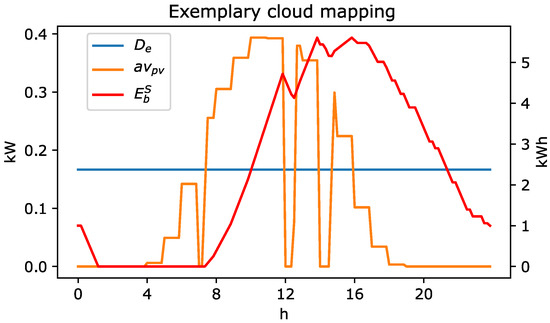
Figure 3.
Exemplary solar radiation time series (yellow line) created by the mapping for randomly sized and randomly distributed clouds. The resulting cost-optimal battery storage levels (red line), which provide for the constant electricity demand (blue line), are shown.
Standardized load profiles for German households [22,23] are used for the heat and electricity demands for the full model in Section 4.4. The time series based on those profiles are scaled to have a total electricity demand equal to the electricity-only model (24 kWh per day). The total heat demand is twice as large as the electricity demand (48 kWh per day). We assume the heat pump to have a coefficient of performance of 3. The heat pump’s power rating is large enough to cover the heat demand in every time step, making the heat storage optional from a pure heat balancing perspective. We use the mapping as described above with randomly distributed clouds and random cloud size.
To deal with the scale heterogeneity of our interpretable features, we normalize them before applying the regression in Equation (1). To normalize the input and interpretable feature vectors, we group their entries. One group contains, for example, all entries in that describe the solar radiation availability time series. We subtract the smallest value from each group member and divide by the largest difference within the group. We define as the normalized versions of and respectively, and as the normalized output values to be explained from the ESD model , in this case, the cost-optimal battery capacities. We then rewrite Equation (1) to create the explanation for the building energy system as
For the distance metric , we use an exponential kernel with a radial basis function on the normalized inputs, i.e.,
with as the normalized input vector at the POI. The vector is the standard deviation of all normalized input variations in the experiment.
For the complexity measurement , we chose the number of non-zero weights of g, allowing only one weight to be non-zero. For the implementation, we choose , with as the weights vector of the linear function g, i.e., . The parameter is increased until has only one non-zero entry. This LASSO path procedure is described in [24]. We will refer to the feature corresponding to this non-zero entry as the most relevant interpretable feature.
The python implementation of our experiments can be found on https://github.com/pe0nd/LIME_for_ESD (accessed on 20 January 2023).
4.3. Explanation Results: Electricity Only
We first omit the heat sector of the exemplary building energy system to facilitate the manual validation of the results. For our exemplary building energy system of a building with a PV power plant, we create an explanation for the cost-optimal battery capacity for two points of interest by comparing the most relevant interpretable features determined by our approach.
The first POI has low specific battery investment costs of 600 €/kWh, a storable PV surplus of 5 kWh, 5 clouds, and a cloud size of 0.5 kWh. We refer to this POI as cheap battery. The input vector for the second POI is identical except for a higher specific battery investment cost of 1200 €/kWh. We refer to this second POI as expensive battery.
Table 2 shows that for cheap battery, the last feature that remains non-zero is the cloud size ; i.e., is the most relevant interpretable feature for explaining the cost-optimal battery capacity at this POI. Applying our approach to the expensive battery results in the PV surplus being the most relevant interpretable feature affecting the cost-optimal battery capacity.
Table 2.
Output of the proposed methodology for the electricity-only ESD model. The most relevant interpretable features for the cost-optimal battery capacity using different cloud mappings are shown. Interpretable features are the cloud size , the number of clouds , the storable PV surplus , specific battery investment costs , and morning mist .
Verifying why the different most relevant interpretable features at each POI is a good explanation considering the different uses for battery storage. First, suppose that the specific costs of battery capacity are high. In this case, building a small battery is cost-optimal to mitigate the fluctuations in electricity production caused by the clouds during the day. The optimal battery capacity for this purpose corresponds to the energy lost by a single cloud. In contrast, if the specific battery investment costs are low compared to the electricity prices, it is cost-optimal to build a large battery. This battery stores electric energy for nighttime, which otherwise would be curtailed from the PV power plant production during the daytime. In this case, the storable PV surplus is the dominant feature for determining the battery capacity.
Table 2 also shows the most relevant interpretable features at the points of interest for different implementations of the mapping function , i.e., fixed or random cloud size and equally or randomly distributed clouds. The most relevant interpretable features are not affected by the different mapping functions. Hence, the explanations for these points of interest are robust against different implementations of the mapping function.
Figure 4 compares our proposed methodology and traditional sensitivity analysis. To this end, we provide in Figure 4a the effect of changes in the solar radiation availability time series on the cost-optimal battery capacity for the POI cheap battery. The top plot shows the sensitivity analysis results for a fixed demand and a deterministic feature mapping with evenly distributed clouds of fixed size. The bottom plot displays the sensitivity results for a standardized load curve, namely demand and randomized cloud placement and size. For the deterministic scenario, the period between 7:40 and 16:00 turns out to be crucial for determining the optimal battery capacity. This is plausible since it is when the PV production exceeds the demand, resulting in surplus PV energy. However, this explanation is not easily deduced from the sensitivity results in the randomized setting. On the other hand, the proposed methodology provides clear and interpretable results as shown in Figure 4b. The fitted linear model provides weights for the interpretable features that are better understandable for both experts and non-experts.
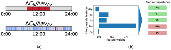
Figure 4.
Comparison of sensitivity analysis and the proposed methodology for explaining the cost-optimal battery capacity at the POI cheap battery. (a): Sensitivity of towards changes in solar radiation availability . Red values indicate a positive sensitivity, and blue values indicate a negative sensitivity. Top: deterministic cloud mapping and constant demand. Bottom: cloud mapping with random cloud sizes , random cloud distribution, and a standardized load profile. (b): Weights of the fitted linear model. Green implies positive influence, and red implies negative influence. The features are ordered by absolute weight magnitude on the right.
4.4. Explanation Results: Including the Heat Sector
We now examine the exemplary building energy system, including the heat sector, i.e., with a heat demand, a heat storage, and a heat pump, and explain the cost-optimal battery capacity and the cost-optimal heat storage capacity . The heat storage can offer temporal flexibility to the system if the heat pump converts excess electricity from the PV power plant into heat. This additional flexibility might allow part of the battery storage to be replaced by heat storage.
We investigate four different points of interest to check if the additional flexibility provided by the heat storage changes the explanation for the cost-optimal battery capacity. All points of interest map to interpretable features with a storable PV surplus of 9 kWh, 5 clouds, and a mean cloud size of 0.5 kWh. We consider a larger storable PV surplus compared to Section 4.3 since the additional heat demand has to be provided by the heat pump, which increases the electricity demand. The examined points of interest differ in their specific battery investment costs and specific heat storage investment costs . We refer to the points of interest by their specific investment costs for heat storage and the battery. The specific heat storage investment costs are either cheap ( €/kWh) or expensive ( = 200 €/kWh). Specific battery investment costs are cheap ( = 600 €/kWh) or expensive ( = 1200 €/kWh).
The most relevant interpretable features determined by our methodology for all POIs are shown in Table 3. The storable PV surplus is the most relevant feature for explaining the cost-optimal heat storage capacity, no matter the specific battery investment cost if heat storage is cheap. The cost-optimal for the points of interest with cheap heat storage is mostly explained by the storable PV surplus or the cloud size , but not the specific heat-storage investment costs . One may anticipate that the specific heat storage investment costs would be the most relevant interpretable feature, as incorporating heat storage with heat pumps presents a more cost-effective way of utilizing electric energy generated by PV production, which could potentially replace battery storage in the exemplary building energy system. However, it is important to note that heat storage is not a complete substitute for battery storage in the exemplary building energy system, as heat cannot be converted back into electricity. As a result, battery storage cannot be fully replaced by heat storage.
Table 3.
The most relevant interpretable features for cost-optimal battery capacity and heat storage capacity . Interpretable features are the cloud size , the number of clouds , the storable PV surplus , specific battery investment costs , morning mist , and specific heat storage investment costs .
For POI expensive battery and expensive heat storage, Table 3 shows that the cloud size is the most relevant interpretable feature for . The storable PV surplus is the most relevant interpretable feature for . At this POI, expensive heat storage is still relatively cheap compared to expensive battery storage. Hence it will be used to store most of the storable PV surplus. Keeping a small battery capacity is cost-optimal for storing electricity fluctuations caused by clouds. The POI expensive heat storage, cheap battery has the specific heat storage investment costs as the most relevant interpretable feature for explaining and . At this POI, the specific investment costs of heat storage capacity and battery capacity are close to balance; i.e., a change in relative investment costs shifts between battery and heat storage.
These examples show that the behavior of even this simple energy system model is not always intuitive. However, our method is able to create explanations in the form of the most relevant interpretable features for and .
5. Experimental Validation: Country-Wide Model
In this section, we employ our approach to create an explanation for different German energy system transition paths towards low-carbon-emitting technologies, e.g., heat pumps and battery electric vehicles (BEVs). Section 5.1 introduces the ESD model used.Next, we define interpretable features in Section 5.2. Finally, we show the explanation created in Section 5.3.
5.1. ESD Model Implementation
We use the German energy system model presented in [5]. The model is based on Germany’s 2016 production capacities and energy demands as an initial condition and takes the heat, electricity, and transport sector into account. The objective function is cost minimization in a time horizon until 2050. We only simulate even years using a sparse time step selection of 8 weeks per simulated year to reduce computation time. Due to linearly decreasing CO limits in all feasible solutions, the initial energy system has to change.
The ESD model has the cost-optimal operation and extension plan as its output. We refer to this cost-optimal extension plan of a technology as its transition path. For comparing different transition paths by a single value, we explain the aggregated use of a technology by its energetic use as modeled years , with as the energy output and t as time and y as years. Note that a technology that is deployed earlier will typically provide more total energy than one that is deployed later, but this could be offset if the later-deployed technology is adopted at a faster rate.
5.2. Interpretable Features
We use three interpretable features: the fossil fuel price, the correlation of PV availability with heat demand, and the correlation of wind availability with heat demand.
The German ESD model uses five fuels: coal, gas, oil, lignite, and biomass. We define a change in fossil fuel price to be the change in prices of all fuels, except biomass; i.e., for a 10% increase in fossil fuel price, the costs of coal, gas, oil, and lignite increase by 10%. Hence, we define the mapping with Y as the number of years of the optimization horizon since prices are fixed within a year in this model.
We define and to map the correlation to the input availability time series of wind and PV, i.e., with T being the set of time steps within a modeled year. The mapping takes the availability time series of wind (or PV) at the POI and alters them to increase or decrease their correlation towards the heat demand without changing their full load hours. First, we determine the correlation of the wind (or PV) availability time series to the heat demand. If the correlation is below the desired level, the time step with the highest heat demand is determined, as well as the time steps with the highest wind (or PV) availability. For the availability time series, the values of those two time steps are switched. Since the highest wind (or PV) availability is now in the same time step as the highest heat demand, the correlation of the two time series increases slightly. We continue this sorting process with the next highest values until the desired correlation, and thus the simultaneity of demand and production availability is reached. If the correlation of an availability time series and the heat demand is above the desired correlation, the lowest heat demand time series is used for the value swapping; i.e., the highest wind (or PV) availability will appear when the heat demand is at its minimum.
The correlation of the wind’s onshore and offshore availability time series with the heat demand at is about 0.2 for both of them. For PV availability at , the correlation with heat demand is about −0.33. We create two variations of the time series each for wind onshore, wind offshore, and PV production availability. The first set of time series created has its correlation increased by 0.2, and the second set of time series has its correlation decreased by 0.2. For the distance metric, we use an exponential kernel as in Equation (4) on the availability time series and the price vector.
5.3. Explanation Results: Energy Transition Paths
Figure 5 shows the cost-optimal heat provision by heat pumps, the cost-optimal transport provided by BEVs, and the cost-optimal electricity production from wind power for different input variations.
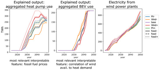
Figure 5.
Yearly energy output of different technologies for different interpretable input variations in the German energy system model. Each line is a different variation with the color encoding the correlation of the PV or wind availability time series to the heat demand and the line style encoding the fossil fuel price. On the left is heat output by heat pumps. In the middle is propulsion output from battery electric vehicles. On the right is electricity output of wind onshore and offshore power plants.
The most relevant interpretable feature for the transition speed towards heat pumps is fossil fuel prices. The importance of fossil fuel prices can be seen in the left graph of Figure 5. For variations with expensive fossil fuel prices, heat pumps are used earlier and to a greater extent than for cheap fossil fuel prices.
This explanation makes sense when considering the available technologies for providing heat within the model. Heat is produced by burning biomass, gas, or oil, or by using electricity to power resistive heaters or heat pumps. Resistive heaters have lower investment costs but are more expensive in the long term compared to heat pumps because of their lower coefficient of performance. Therefore, when fossil fuel prices rise, the cost-optimal solution to meet the heat demand is heat pumps. Additionally, electricity produced by wind power plants can be used more efficiently by heat pumps when wind power production is better aligned with heat demand; however, this effect is weaker than the fossil fuel price change.
The transportation energy provided by BEV for different input variations is shown in the center graph of Figure 5. The most relevant interpretable feature for explaining the transition towards BEVs is the correlation between wind power availability and heat demand. If the wind power availability is less correlated with the heat demand, a transition towards BEV happens earlier. If the wind power availability is correlated more with the heat demand, the transition happens in later years.
It may seem counterintuitive that less simultaneity between wind power production and heat demand would impact the transport sector, but it makes sense. When wind power, the cheapest source of renewable energy in this model, is less able to provide the required heat, more heat is generated by burning fossil fuels. This leads to an increase in CO emissions. The additional CO emissions needed for heating require savings in other sectors, as emissions must be kept below their limit. This explains an earlier transition to battery-electric vehicles (BEVs) away from combustion vehicles, as the transport sector is the cheapest option for reducing emissions in this setup. Furthermore, the right graph of Figure 5 shows that large capacities of wind power plants are built in later years of the model, even when the simultaneity of wind availability with heat demand is low. This indicates the need for CO reduction.
6. Discussion
The proposed method of creating explanations using LIME-based methodology offers several benefits compared to sensitivity analysis, which is commonly used to explain optimization results. First, the number of explaining factors is significantly reduced. This is beneficial for discussion with experts and non-experts. Second, the sensitivity results for each individual input dimension make it non-trivial to extract the underlying determining reasons. For example, considering the setup in Figure 4, the color map derived from sensitivity analysis could hardly encode factors such as cloud size in an obvious fashion. The third argument concerns computation times and ease of implementation. While sensitivity analysis for linear programs can be made efficient by exploiting the KKT optimality conditions [25], this is not implemented or easily accessible in many existing ESD frameworks. If sensitivities for high-dimensional inputs then have to be computed externally via numeric differentiation, the effort quickly becomes infeasible. In contrast, for the proposed methodology, the effort can be adapted by changing the number of selected interpretable features and the number of parameter variations used.
When transferring the concept of LIME to energy systems, two challenges arise that have to be considered by domain experts: defining interpretable features and choosing the proper distance metric between different input variations. The definition of interpretable features is challenging since they have to be independent of one another. Dependent interpretable features will also be related in an explanation. For example, consider the exemplary building energy system from Section 4.3 and the POI with low battery investment costs. Instead of the storable PV surplus, we use the total energy availability of the PV power plant as an interpretable feature. The explanation for the cost-optimal battery capacity will equally depend on cloud size, the number of clouds, and the total energy output availability since the energy output is affected by the number of clouds times the cloud size.
The distance metric weights the changes in the interpretable features based on the changes in the actual model inputs. For machine learning classifiers, model inputs are homogeneous; e.g., all inputs of an image classifier are pixels. The distance between interpretable variations can be determined by summing up the distance between individual input changes. However, finding an appropriate distance metric remains a challenge, as noted in [26]. For energy system models, the inputs are heterogeneous, e.g., cost parameters that are part of the model’s objective function or availability time series in the model’s constraints. Interpretable features that affect multiple constraints, such as by altering an availability time series, are considered more distant than those that affect only a single parameter of the objective because their input distances are simply summed. However, it should be noted that the objective often has a greater impact on the model’s outcome than changes in the constraints, which is not considered by the distance metric. Investigating the effect of different distance metrics on the stability of the explanation could be an interesting area for future research.
7. Conclusions
In this paper, we propose a methodology based on LIME [15] that can be applied to bottom-up ESD models, creating explanations beyond the scope of sensitivity analysis. We applied the idea of an interpretable feature space from LIME to our approach. We mapped interpretable features to the model’s inputs and allowed explanations based on those features instead of the model’s inputs. The proposed methodology automatically selects the interpretable features that are most important for an explanation. The complexity of an explanation, i.e., the number of relevant interpretable features, is a parameter of choice, allowing one to choose an appropriate degree of explanation complexity suited for different target groups. Overall, the use of interpretable features makes explanations more straightforward to understand by non-experts and, therefore, could support them in making decisions.
The shown methodology faces some challenges that might be addressed in future works. Those challenges are the mapping of interpretable features to the heterogeneous inputs of the ESD models and finding the appropriate distance metric for input variations. Additionally, the idea behind LIME’s interpretable abstraction layer can be applied to a range of other contexts that give deeper insights into feature influence, such as partial dependency plots [26].
Author Contributions
Conceptualization, J.H. and F.S.; methodology, J.H.; software, J.H.; validation, J.H.; investigation, J.H.; resources, J.H.; writing—original draft preparation, J.H.; writing—review and editing, J.B. and F.S.; visualization, J.H.; supervision, F.S.; project administration, F.S.; funding acquisition, F.S. All authors have read and agreed to the published version of the manuscript.
Funding
This work was funded by the German Federal Ministry of Education and Research (Bundesministerium für Bildung und Forschung BMBF) in the Project PlexPlain—Explainable AI for complex linear programs on the example of intelligent energy systems, funding number 01|S19081.
Acknowledgments
We acknowledge support by the Deutsche Forschungsgemeinschaft (DFG, German Research Foundation) and the Open Access Publishing Fund of Technical University of Darmstadt.
Conflicts of Interest
The authors declare no conflict of interest. The funders had no role in the design of the study; in the collection, analyses, or interpretation of data; in the writing of the manuscript; or in the decision to publish the results.
Sample Availability
A Python implementation of the running example is available at https://github.com/pe0nd/LIME_for_ESD (accessed on 20 January 2023).
Abbreviations
The following abbreviations are used in this manuscript:
| BEV | battery electric vehicle |
| ESD | energy system design |
| LIME | local interpretable model-agnostic explanation |
| PV | photo-voltaic |
| POI | point of interest |
Appendix A
In this supplementary section, we present the technical details of the building energy system model used as a running example in the main paper. Below are the equations for the simple PV house energy system. The equations are a modified version of the equations from [7]. Blue variables or equations are only present if the model considers the heat sector.
The objective of the energy system is to minimize system costs. The system costs consist of operational costs for buying energy and investment costs for the battery capacity and heat storage capacity , respectively, at price , , and .
Note that the PV and heat pump capacity is assumed to be fixed and thus is not part of the objective function.
A set of constraints restricts the objective. The first constraint is the electric power balance of the system,
On the left side of the equation is the energy provided by the PV power plant , the energy taken from the battery storage , and the energy bought from the grid . On the right side is the energy demand , the energy put into the battery and the electricity consumption of the heat pump . Both sides of the equation must be balanced for every time step t to ensure that the electricity supply equals the demand. Like the electric power balance, a heat power balance constraint is defined for every time step t if the energy system considers the heat sector.
with as the heat output of the heat pump, as the heat taken from the heat storage, as the heat demand, and as the heat put into the heat storage.
The battery storage level is defined by
where the current energy stored in the battery is given by the energy in the previous time step reduced by the energy taken from the battery and increased by the energy added in the current time step . A power inverter loss is considered for the battery storage by applying a loss to the energy stored in the battery. We chose to be 0.95 to represent an inverter loss of 5%. The upper and lower limits of the battery level are defined as
For heat storage, the same logic is applied to the battery.
the current Energy stored in the heat storage is given by the energy stored at the previous time step decreased by the heat taken from the storage and increased by the energy added to the storage . It is assumed that part of the heat stored is lost every time step, which is described by . We chose to represent a heat loss of 1% per hour of the energy stored. The heat storage is restricted by its capacity and an additional bound on the maximum storage size that can be installed.
We chose to be 46.6 kWh or 1 m of water with a maximum heat difference of 40 °K. In order to prevent storage depletion of the battery and the heat storage at the end of the optimized time interval, we define as the time step prior to in Equations (A4) and (A6).
In this energy system, the PV capacity is an input parameter, not part of the optimization. Hence, the PV energy production can be described with the time series . The time series limits the possible energy output at each time step, i.e., a percentage of output at each time step times the PV capacity.
The limits of the heat pump are defined as
where is the heat output and is the electricity consumption of the heat pump. The heat output of the heat pump is bound by the electricity consumption times the coefficient of performance of the pump. We chose a of 3 in our experiments. Furthermore, we assume that the heat pump’s power is limited by twice the highest heat demand value . This limitation was made to prevent production spikes since there are no costs for the heat pump’s capacity.
Finally, selling energy to the grid is not considered in this model. Hence, the energy bought is limited to be positive by the following equation.
References
- Loulou, R.; Remme, U.; Kanudia, A.; Lehtila, A.; Goldstein, G. Documentation for the Times Model Part II; Energy Technology Systems Analysis Programme; International Energy Agency: Paris, France, 2005. [Google Scholar]
- Howells, M.; Rogner, H.; Strachan, N.; Heaps, C.; Huntington, H.; Kypreos, S.; Hughes, A.; Silveira, S.; DeCarolis, J.; Bazillian, M.; et al. OSeMOSYS: The open source energy modeling system: An introduction to its ethos, structure and development. Energy Policy 2011, 39, 5850–5870. [Google Scholar] [CrossRef]
- TemoaProject. Open Energy Outlook for the United States. Available online: https://github.com/TemoaProject/oeo (accessed on 4 March 2022).
- Calliope-Project. Model of the UK Power System Built with Calliope. Available online: https://github.com/calliope-project/uk-calliope (accessed on 4 March 2022).
- Barbosa, J.; Ripp, C.; Steinke, F. Accessible Modeling of the German Energy Transition: An Open, Compact, and Validated Model. Energies 2021, 14, 8084. [Google Scholar] [CrossRef]
- Weber, J.; Heinrichs, H.U.; Gillessen, B.; Schumann, D.; Hörsch, J.; Brown, T.; Witthaut, D. Counter-intuitive behaviour of energy system models under CO2 caps and prices. Energy 2019, 170, 22–30. [Google Scholar] [CrossRef]
- Hülsmann, J.; Steinke, F. Explaining Complex Energy Systems: A Challenge. In Proceedings of the Workshop: Tackling Climate Change with ML, 34th Conference on Neural Information Processing Systems (NeurIPS 2020), Vancouver, BC, Canada, 6–12 December 2020. [Google Scholar]
- Christopher Frey, H.; Patil, S.R. Identification and review of sensitivity analysis methods. Risk Anal. 2002, 22, 553–578. [Google Scholar] [CrossRef]
- Tian, W. A review of sensitivity analysis methods in building energy analysis. Renew. Sustain. Energy Rev. 2013, 20, 411–419. [Google Scholar] [CrossRef]
- Rezzouk, H.; Mellit, A. Feasibility study and sensitivity analysis of a stand-alone photovoltaic-diesel-battery hybrid energy system in the north of Algeria. Renew. Sustain. Energy Rev. 2015, 43, 1134–1150. [Google Scholar] [CrossRef]
- Sun, Y. Sensitivity analysis of macro-parameters in the system design of net zero energy building. Energy Build. 2015, 86, 464–477. [Google Scholar] [CrossRef]
- Nurunnabi, M.; Roy, N.K.; Hossain, E.; Pota, H.R. Size optimization and sensitivity analysis of hybrid wind/PV micro-grids-a case study for Bangladesh. IEEE Access 2019, 7, 150120–150140. [Google Scholar] [CrossRef]
- Bazaraa, M.S.; Jarvis, J.J.; Sherali, H.D. Linear Programming and Network Flows; John Wiley & Sons: Hoboken, NJ, USA, 2008. [Google Scholar]
- Holzinger, A.; Biemann, C.; Pattichis, C.S.; Kell, D.B. What do we need to build explainable AI systems for the medical domain? arXiv 2017, arXiv:1712.09923. [Google Scholar]
- Ribeiro, M.T.; Singh, S.; Guestrin, C. “Why should I trust you?” Explaining the predictions of any classifier. In Proceedings of the 22nd ACM SIGKDD International Conference on Knowledge Discovery and Data Mining, San Francisco, CA, USA, 13–17 August 2016; pp. 1135–1144. [Google Scholar]
- Fan, C.; Xiao, F.; Yan, C.; Liu, C.; Li, Z.; Wang, J. A novel methodology to explain and evaluate data-driven building energy performance models based on interpretable machine learning. Appl. Energy 2019, 235, 1551–1560. [Google Scholar] [CrossRef]
- Chen, M.; Liu, Q.; Chen, S.; Liu, Y.; Zhang, C.H.; Liu, R. XGBoost-based algorithm interpretation and application on post-fault transient stability status prediction of power system. IEEE Access 2019, 7, 13149–13158. [Google Scholar] [CrossRef]
- Chaibi, M.; Benghoulam, E.; Tarik, L.; Berrada, M.; Hmaidi, A.E. An interpretable machine learning model for daily global solar radiation prediction. Energies 2021, 14, 7367. [Google Scholar] [CrossRef]
- Machlev, R.; Heistrene, L.; Perl, M.; Levy, K.; Belikov, J.; Mannor, S.; Levron, Y. Explainable Artificial Intelligence (XAI) techniques for energy and power systems: Review, challenges and opportunities. Energy AI 2022, 9, 100169. [Google Scholar] [CrossRef]
- Herbst, A.; Toro, F.; Reitze, F.; Jochem, E. Introduction to energy systems modelling. Swiss J. Econ. Stat. 2012, 148, 111–135. [Google Scholar] [CrossRef]
- Pfenninger, S.; Staffell, I. Renewables.ninja. Available online: https://www.renewables.ninja/ (accessed on 4 March 2022).
- BDEW, Bundesverband der Energie-und Wasserwirtschaft. Standartlastprofile Gas. Available online: https://www.bdew.de/energie/standardlastprofile-gas/ (accessed on 15 March 2022).
- BDEW, Bundesverband der Energie-und Wasserwirtschaft. Standartlastprofile Strom. Available online: https://www.bdew.de/energie/standardlastprofile-strom/ (accessed on 15 March 2022).
- Efron, B.; Hastie, T.; Johnstone, I.; Tibshirani, R. Least angle regression. Ann. Stat. 2004, 32, 407–499. [Google Scholar] [CrossRef]
- Fang, S.C.; Puthenpura, S. Linear Optimization and Extensions: Theory and Algorithms; Prentice-Hall, Inc.: Hoboken, NJ, USA, 1993. [Google Scholar]
- Molnar, C. Interpretable Machine Learning—A Guide for Making Black Box Models Explainable, 2nd ed.; Bookdown: Sheffield, UK, 2022. [Google Scholar]


Disclaimer/Publisher’s Note: The statements, opinions and data contained in all publications are solely those of the individual author(s) and contributor(s) and not of MDPI and/or the editor(s). MDPI and/or the editor(s) disclaim responsibility for any injury to people or property resulting from any ideas, methods, instructions or products referred to in the content. |
© 2023 by the authors. Licensee MDPI, Basel, Switzerland. This article is an open access article distributed under the terms and conditions of the Creative Commons Attribution (CC BY) license (https://creativecommons.org/licenses/by/4.0/).