
Thermogram Based Indirect Thermographic Temperature Measurement of Reactive Power Compensation Capacitors


Abstract
:1. Introduction
2. Materials and Methods
2.1. Dimensions and Internal Structure of the Capacitor
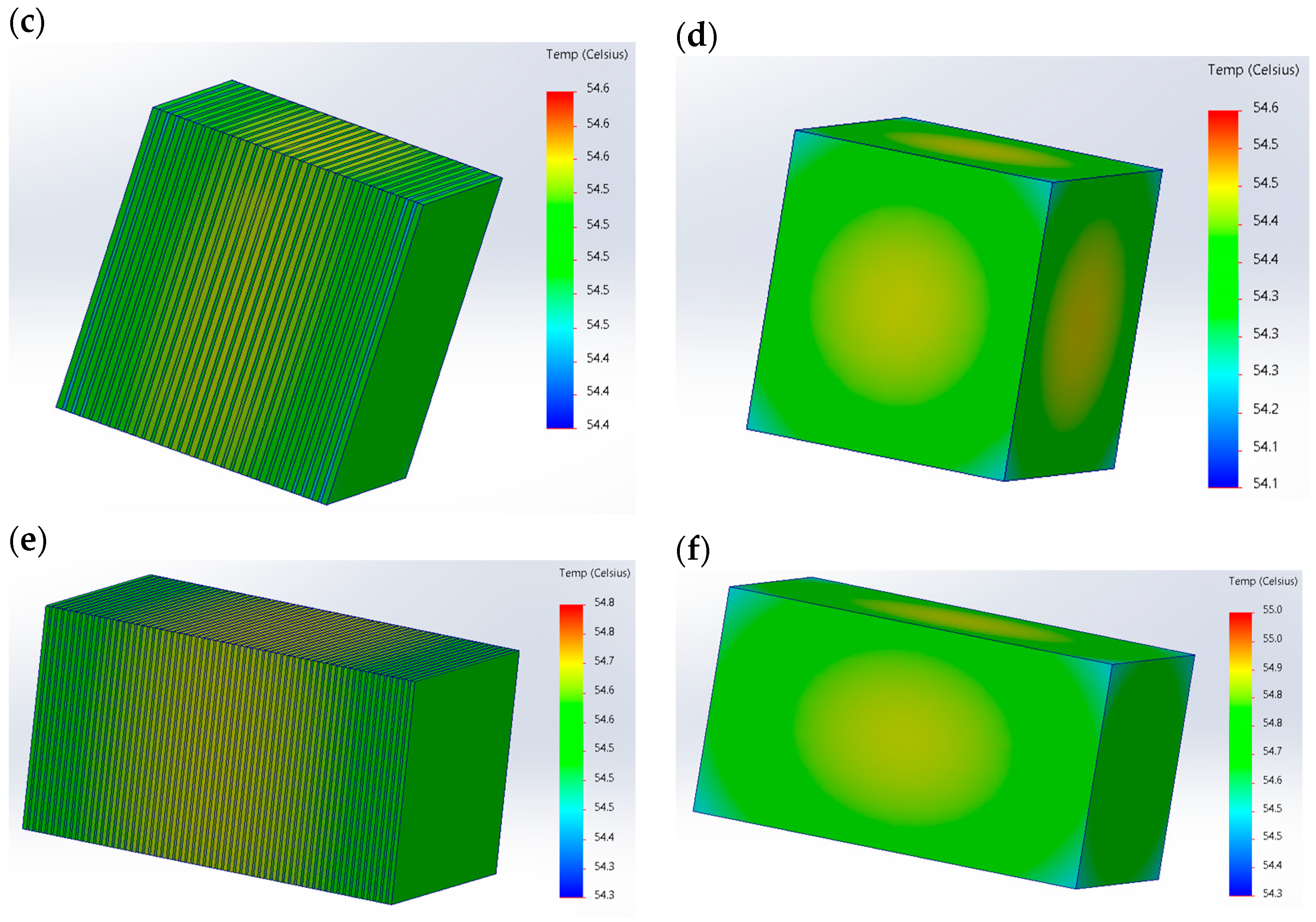
2.2. Modeling the Temperature Distribution Inside the Capacitor
2.3. Verification of the Received Model
3. Results
4. Discussion
5. Conclusions
Author Contributions
Funding
Data Availability Statement
Conflicts of Interest
Nomenclature
| T | Temperature |
| λ | Wavelength |
| ε | Emissivity coefficient |
| Tr | Reflected temperature |
| d | Distance between the lens and the observed object |
| Ta | Ambient (air) temperature |
| τa | Transmittance of the atmosphere |
| Tl | Temperature of the external optical system |
| τl | Transmittance of the external optical system |
| ω | Relative humidity |
| β | Viewing angle |
| Tus | Sharpness of the recorded thermogram |
| hr | Radiation coefficient |
| σc | Stefan–Boltzmann constant |
| TS | Surface temperature |
| hc | Convection coefficient |
| hcr | Convection coefficient for a cylindrical surface |
| dr | Roll diameter |
| Pr | Prandtl number |
| α | Coefficient of expansion |
| ν | Kinematic viscosity |
| c | Specific heat |
| η | Dynamic air viscosity |
| k | Thermal conductivity |
| hcf | Convection coefficient for a flat surface |
| Nu | Nusselt number |
| L | Characteristic length in meters |
| a, b, alam, blam, aturb, bturb | Coefficients |
| Gr | Grashof number |
| ρ | Air density |
| r | Reflectance factor |
| Tc | Thermographic measurement of temperature |
| Tcs | Surface temperature of the capacitor obtained as a result of the simulation work |
| Tt | Temperature measured with a thermocouple |
| Tts | Temperature obtained as a result of simulation work for the location of the thermocouple |
| Trs | Temperature of the point inside the case |
| Power dissipated inside capacitor | |
| d1 | External capacitor dimension |
| d1 | Internal capacitor dimension |
| l | Capacitor high |
References
- Qiao, X.; Bian, J.; Chen, C.; Li, H. Comparison and Analysis of Reactive Power Compensation Strategy in Power System. In Proceedings of the IEEE Sustainable Power and Energy Conference (iSPEC), Beijing, China, 21–23 November 2019; pp. 689–692. [Google Scholar] [CrossRef]
- Chen, Y.; Zhao, X.; Yang, Y.; Shi, Y. Online Diagnosis of Inter-turn Short Circuit for Dual-Redundancy Permanent Magnet Synchronous Motor Based on Reactive Power Difference. Energies 2019, 12, 510. [Google Scholar] [CrossRef] [Green Version]
- Tariq, H.; Czapp, S.; Tariq, S.; Cheema, K.M.; Hussain, A.; Milyani, A.H.; Alghamdi, S.; Elbarbary, Z.M.S. Comparative Analysis of Reactive Power Compensation Devices in a Real Electric Substation. Energies 2022, 15, 4453. [Google Scholar] [CrossRef]
- Graña-López, M.A.; García-Diez, A.; Filgueira-Vizoso, A.; Chouza-Gestoso, J.; Masdías-Bonome, A. Study of the Sustainability of Electrical Power Systems: Analysis of the Causes that Generate Reactive Power. Sustainability 2019, 11, 7202. [Google Scholar] [CrossRef] [Green Version]
- Yani, A.; Junaidi, J.; Irwanto, M.; Haziah, A.H. Optimum reactive power to improve power factor in industry using genetic algortihm. Indones. J. Electr. Eng. Comput. Sci. 2019, 14, 751–757. [Google Scholar] [CrossRef]
- Van Huyen, D.; Thanh Hien, P.; Cuong, N.D. Design of Dynamic—Static VAr compensation based on microcontroller for improving power factor. In Proceedings of the 2017 International Conference on System Science and Engineering (ICSSE), Ho Chi Minh City, Vietnam, 21–23 July 2017; pp. 186–190. [Google Scholar] [CrossRef]
- Ernst, S.; Kotulski, L.; Lerch, T.; Rad, M.; Sędziwy, A.; Wojnicki, I. Application of reactive power compensation algorithm for large-scale street lighting. J. Comput. Sci. 2021, 51, 101338–101346. [Google Scholar] [CrossRef]
- Kien, L.C.; Hien, C.T.; Nguyen, T.T. Optimal Reactive Power Generation for Transmission Power Systems Considering Discrete Values of Capacitors and Tap Changers. Appl. Sci. 2021, 11, 5378. [Google Scholar] [CrossRef]
- Umran, H.M.; Wang, F.; He, Y. Ageing: Causes and Effects on the Reliability of Polypropylene Film Used for HVDC Capacitor. IEEE Access 2020, 8, 40413–40430. [Google Scholar] [CrossRef]
- Karimi, D.; Khaleghi, S.; Behi, H.; Beheshti, H.; Hosen, M.S.; Akbarzadeh, M.; Van Mierlo, J.; Berecibar, M. Lithium-Ion Capacitor Lifetime Extension through an Optimal Thermal Management System for Smart Grid Applications. Energies 2021, 14, 2907. [Google Scholar] [CrossRef]
- Brown, R.W. Linking corrosion and catastrophic failure in low-power metallized polypropylene capacitors. IEEE Trans. Device Mater. Reliab. 2006, 6, 326–333. [Google Scholar] [CrossRef]
- Sharma, P.K.; Bhargava, C.; Kotecha, K. Sustainability Analysis of a ZnO-NaCl-Based Capacitor Using Accelerated Life Testing and an Intelligent Modeling Approach. Sustainability 2021, 13, 10736. [Google Scholar] [CrossRef]
- Reed, C.W.; Cichanowskil, S.W. The fundamentals of aging in HV polymer-film capacitors. IEEE Trans. Dielectr. Electr. Insul. 1994, 1, 904–922. [Google Scholar] [CrossRef]
- Ritamäki, M.; Rytöluoto, I.; Lahti, K. Performance metrics for a modern BOPP capacitor film. IEEE Trans. Dielectr. Electr. Insul. 2019, 26, 1229–1237. [Google Scholar] [CrossRef]
- Andersson, C.; Kristensen, O.; Miller, S.; Gloor, T.; Iannuzzo, F. Lock-in Thermography Failure Detection on Multilayer Ceramic Capacitors After Flex Cracking and Temperature–Humidity–Bias Stress. IEEE J. Emerg. Sel. Top. Power Electron. 2018, 6, 2254–2261. [Google Scholar] [CrossRef] [Green Version]
- Thermocouple Accurancy. Available online: https://mera-sp.pl/akcesoria/1257-sonda-kablowa-18m-zakres-200-180c-termopara-typ-t.htmlhttps://mera-sp.pl/akcesoria/1257-sonda-kablowa-18m-zakres-200-180c-termopara-typ-t.html (accessed on 24 January 2023).
- Thermoresistor PT 1000 Accurancy. Available online: https://www.tme.eu/Document/67cf717905f835bc5efcdcd56ca3a8e2/Pt1000-550_EN.pdf (accessed on 24 January 2023).
- Thermocouple Temperature Transmitter. Available online: https://statinst.com/index.php?route=product/product&product_id=83 (accessed on 24 January 2023).
- Stoynova, A.; Bonev, B.; Brayanov, N. Thermographic Approach for Reliability Estimation of PCB. In Proceedings of the 2018 41st International Spring Seminar on Electronics Technology (ISSE), Zlatibor, Serbia, 16–20 May 2018; pp. 1–7. [Google Scholar] [CrossRef]
- Flir E50. Available online: https://docs.rs-online.com/ca3e/0900766b81371810.pdf (accessed on 24 January 2023).
- Zaccara, M.; Edelman, J.B.; Cardone, G. A general procedure for infrared thermography heat transfer measurements in hypersonic wind tunnels. Int. J. Heat Mass Transf. 2020, 163, 120419–120435. [Google Scholar] [CrossRef]
- Altenburg, S.J.; Straße, A.; Gumenyuk, A.; Maierhofer, C. In-situ monitoring of a laser metal deposition (LMD) process: Comparison of MWIR, SWIR and high-speed NIR thermography. Quant. InfraRed Thermogr. J. 2020, 19, 97–114. [Google Scholar] [CrossRef]
- Yoon, S.T.; Park, J.C. An experimental study on the evaluation of temperature uniformity on the surface of a blackbody using infrared cameras. Quant. InfraRed Thermogr. J. 2021, 19, 172–186. [Google Scholar] [CrossRef]
- Schuss, C.; Remes, K.; Leppänen, K.; Saarela, J.; Fabritius, T.; Eichberger, B.; Rahkonen, T. Detecting Defects in Photovoltaic Cells and Panels with the Help of Time-Resolved Thermography under Outdoor Environmental Conditions. In Proceedings of the 2020 IEEE International Instrumentation and Measurement Technology Conference (I2MTC), Dubrovnik, Croatia, 25–28 May 2020; pp. 1–6. [Google Scholar] [CrossRef]
- Chakraborty, B.; Sinha, B.K. Process-integrated steel ladle monitoring, based on infrared imagin—A robust approach to avoid ladle breakout. Quant. InfraRed Thermogr. J. 2020, 17, 169–191. [Google Scholar] [CrossRef]
- Tomoyuki, T. Coaxiality Evaluation of Coaxial Imaging System with Concentric Silicon–Glass Hybrid Lens for Thermal and Color Imaging. Sensors 2020, 20, 5753. [Google Scholar] [CrossRef]
- Wollack, J.E.; Cataldo, G.; Miller, K.H.; Quijada, A.M. Infrared properties of high-purity silicon. Opt. Lett. 2020, 45, 4935–4938. [Google Scholar] [CrossRef]
- Singh, J.; Arora, A.S. Effectiveness of active dynamic and passive thermography in the detection of maxillary sinusitis. Quant. InfraRed Thermogr. J. 2020, 18, 213–225. [Google Scholar] [CrossRef]
- Dziarski, K.; Hulewicz, A. Effect of unsharpness on the result of thermovision diagnostics of electronic components. In Proceedings of the 15th Quantitative InfraRed Thermography Conference, Porto, Portugal, 6–10 July 2020. [Google Scholar] [CrossRef]
- Dziarski, K.; Hulewicz, A.; Dombek, G. Thermographic Measurement of the Temperature of Reactive Power Compensation Capacitors. Energies 2021, 14, 5736. [Google Scholar] [CrossRef]
- Xu, J.; Wang, X.; Shi, H.; Mei, X. Multi-scale short circuit resistance estimation method for series connected battery strings. Energy 2020, 202, 117647. [Google Scholar] [CrossRef]
- Valdivieso, C.A.; Meunier, G.; Ramdane, B.; Gyselinck, J.; Guerin, C.; Sabariego, R.V. Time-Domain Finite-Element Eddy-Current Homogenization of Windings Using Foster Networks and Recursive Convolution. IEEE Trans. Magn. 2020, 56, 7401408. [Google Scholar] [CrossRef]
- Sato, Y.; Shimotani, T.; Igarashi, H. Synthesis of Cauer-Equivalent Circuit Based on Model Order Reduction Considering Nonlinear Magnetic Property. IEEE Trans. Magn. 2017, 53, 1100204. [Google Scholar] [CrossRef]
- FEM. Available online: https://books.google.pl/books?hl=pl&lr=&id=CExVEAAAQBAJ&oi=fnd&pg=PP1&dq=FEM+method+description&ots=m_E3-szsOk&sig=kutWOtMCIo78jyjzQOecmxF0qiQ&redir_esc=y#v=onepage&q=FEM%20method%20description&f=false (accessed on 7 February 2023).
- Gao, J.; Xiao, M.; Zhang, Y.; Gao, L. A comprehensive review of isogeometric topology optimization: Methods, applications and prospects. Chin. J. Mech. Eng. 2020, 33, 87. [Google Scholar] [CrossRef]
- Capacitor. Available online: https://www.tme.eu/Document/093111ad30aae76bee6b76af6ef3cf17/SR-Passives_KJF-eng.pdf (accessed on 7 February 2023).
- Motic Images Plus 3.0. Available online: https://www.motic.com/As_News/n325.html (accessed on 7 February 2023).
- Alisibramulisi, A. Finite Element Analysis (FEA) Project in Structural Engineering Subject. In Proceedings of the 2019 IEEE 11th International Conference on Engineering Education (ICEED), Kanazawa, Japan, 6–7 November 2019. [Google Scholar] [CrossRef]
- Incropera, F.; De Witt, D. Introduction to Heat Transfer; Wiley: New York, NY, USA, 1985; Available online: https://scirp.org/reference/referencespapers.aspx?referenceid=1503886 (accessed on 29 January 2023).
- Shams Ghahfarokhi, P.; Podgornovs, A.; Kallaste, A.; Cardoso, A.J.M.; Belahcen, A.; Vaimann, T.; Asad, B.; Tiismus, H. Determination of Heat Transfer Coefficient from Housing Surface of a Totally Enclosed Fan-Cooled Machine during Passive Cooling. Machines 2021, 9, 120. [Google Scholar] [CrossRef]
- Li, B. Investigation and modelling of work roll temperature in induction heating by finite element method. J. S. Afr. Inst. Min. Metall. 2018, 118, 735–743. [Google Scholar] [CrossRef]
- Khrapak, S.; Khrapak, A. Prandtl Number in Classical Hard-Sphere and One-Component Plasma Fluids. Molecules 2021, 26, 821. [Google Scholar] [CrossRef]
- Staton, D.A.; Cavagnino, A. Convection heat transfer and flow calculations suitable for electric machines thermal models. IEEE Trans. Ind. Electron. 2008, 55, 3509–3516. [Google Scholar] [CrossRef] [Green Version]
- Ghahfarokhi, P.S. Determination of Forced Convection Coefficient over a Flat Side of Coil. In Proceedings of the 2017 IEEE 58th International Scientific Conference on Power and Electrical Engineering of Riga Technical University (RTUCON), Riga, Latvia, 12–13 October 2017. [Google Scholar] [CrossRef]
- Dziarski, K.; Hulewicz, A.; Dombek, G.; Drużyński, Ł. Indirect Thermographic Temperature Measurement of a Power-Rectifying Diode Die. Energies 2022, 15, 3203. [Google Scholar] [CrossRef]
- Optris Thermographic Camera. Available online: https://www.optris.global/optris-xi-400?gclid=CjwKCAiAoL6eBhA3EiwAXDom5iDyJ7ANskvy59t3eZIY5ngbPO7LCh2NPJaQ94OcHAQARnbD_K9rxxoCSbkQAvD_BwE (accessed on 24 January 2023).
- Kawor, E.T.; Mattei, S. Emissivity measurements for nexel velvet coating 811-21 between −36 °C and 82 °C, 15 ECTP Proceedings. High Temp.—High Press. 1999, 31, 551–556. [Google Scholar] [CrossRef]


| Shape | Gr·Pr | alam | blam | aturb | bturb |
|---|---|---|---|---|---|
| Vertical flat wall | 109 | 0.59 | 0.25 | 0.129 | 0.33 |
| Upper flat wall | 108 | 0.54 | 0.25 | 0.14 | 0.33 |
| Lower flat wall | 105 | 0.25 | 0.25 | NA | NA |
| The Part of the Capacitor | Material | k W/(m·K) | The Range of the Used k Values * W/(m K) | hcf, hcr (−) |
|---|---|---|---|---|
| Case | Aluminum | 200 | 190–230 | 4.27 |
| Plastic caps (outside) | Plastic | 0.54 | 0.41–0.59 | 14.55 |
| Plastic caps | Plastic | 0.54 | 0.41–0.59 | - |
| Electrolyte | Polyurethane | 0.3 | 0.24–0.38 | - |
| Zinc-sprayed | Zinc | 116 | 104–119 | - |
| Roller (metal foil) | Aluminum | 200 | 190–230 | - |
| Roller (plastic) | Polypropylene | 0.2 | 0.18–0.33 | - |
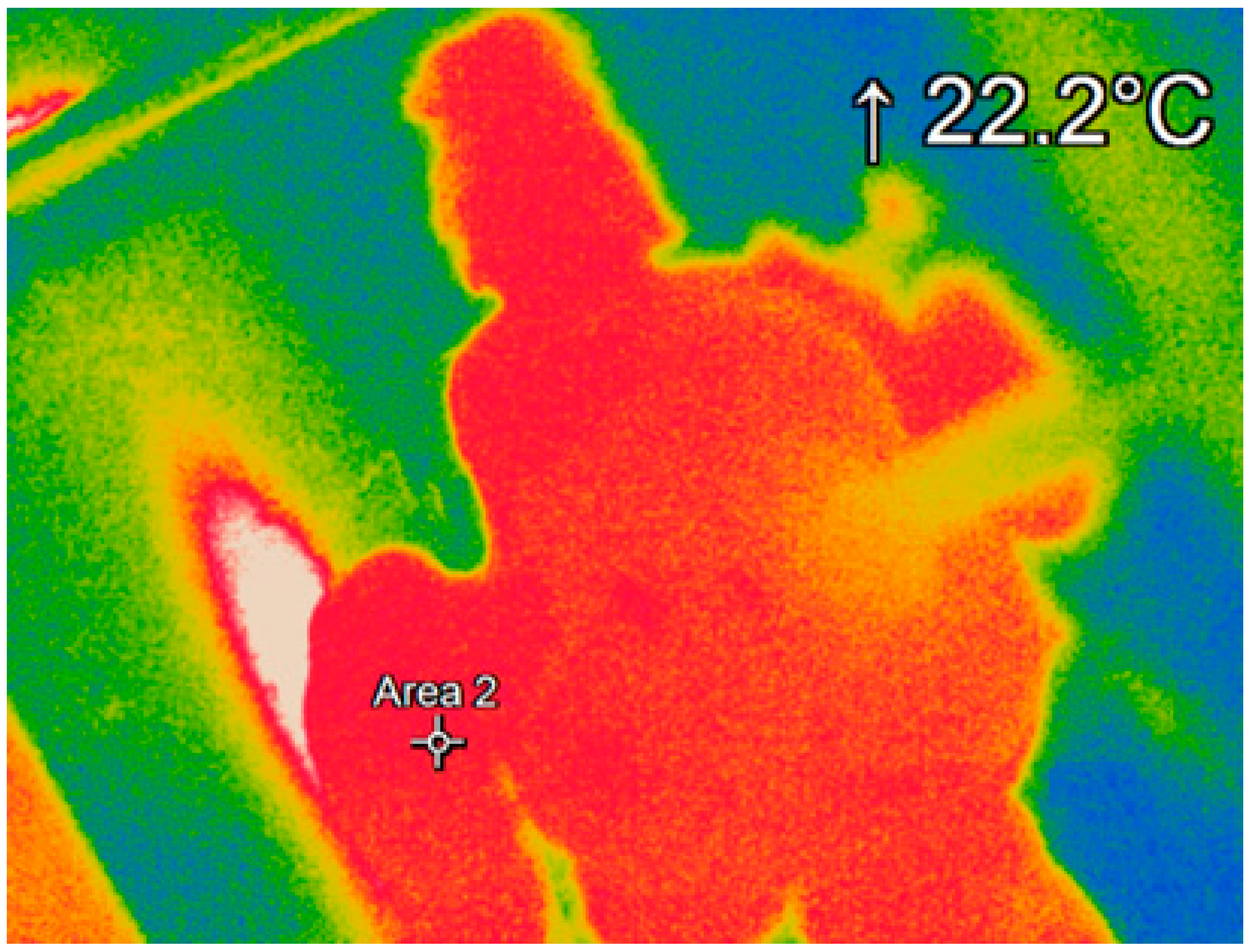
| Tc (°C) | Tcs (°C) | Tc − Tcs (°C) | Tt (°C) | Tts (°C) | Tt − Tts (°C) |
|---|---|---|---|---|---|
| 22.2 | 22.1 | 0.1 | 22.0 | 22.2 | 0.2 |
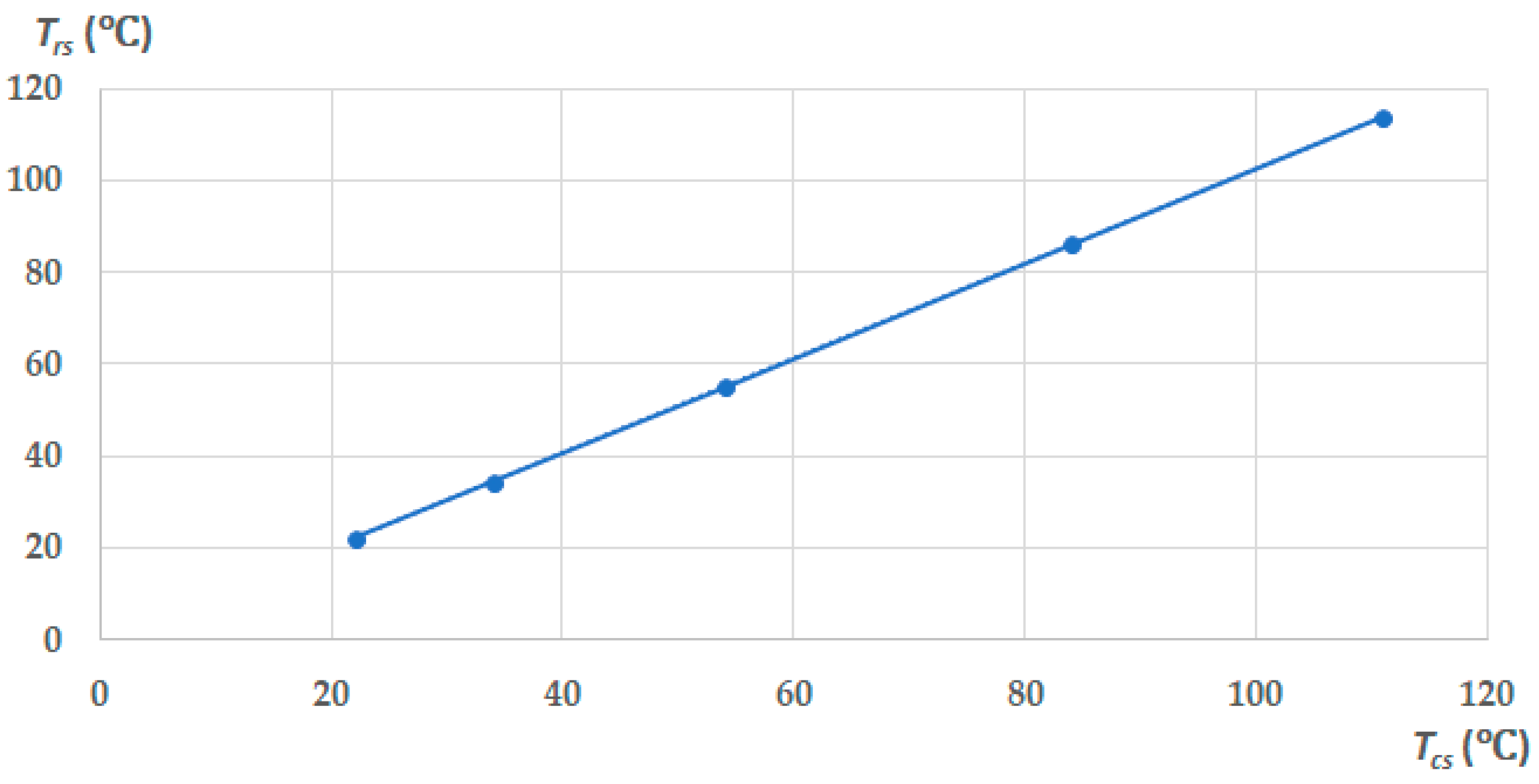
| Tcs (°C) | Trs (°C) | Tcs (°C) | Trs (°C) | Tcs (°C) | Trs (°C) |
|---|---|---|---|---|---|
| 22.0 | 22.2 | 34.0 | 34.5 | 54.0 | 55.1 |
Disclaimer/Publisher’s Note: The statements, opinions and data contained in all publications are solely those of the individual author(s) and contributor(s) and not of MDPI and/or the editor(s). MDPI and/or the editor(s) disclaim responsibility for any injury to people or property resulting from any ideas, methods, instructions or products referred to in the content. |
© 2023 by the authors. Licensee MDPI, Basel, Switzerland. This article is an open access article distributed under the terms and conditions of the Creative Commons Attribution (CC BY) license (https://creativecommons.org/licenses/by/4.0/).
Share and Cite
Hulewicz, A.; Dziarski, K.; Drużyński, Ł.; Dombek, G. Thermogram Based Indirect Thermographic Temperature Measurement of Reactive Power Compensation Capacitors. Energies 2023, 16, 2164. https://doi.org/10.3390/en16052164
Hulewicz A, Dziarski K, Drużyński Ł, Dombek G. Thermogram Based Indirect Thermographic Temperature Measurement of Reactive Power Compensation Capacitors. Energies. 2023; 16(5):2164. https://doi.org/10.3390/en16052164
Chicago/Turabian StyleHulewicz, Arkadiusz, Krzysztof Dziarski, Łukasz Drużyński, and Grzegorz Dombek. 2023. "Thermogram Based Indirect Thermographic Temperature Measurement of Reactive Power Compensation Capacitors" Energies 16, no. 5: 2164. https://doi.org/10.3390/en16052164
APA StyleHulewicz, A., Dziarski, K., Drużyński, Ł., & Dombek, G. (2023). Thermogram Based Indirect Thermographic Temperature Measurement of Reactive Power Compensation Capacitors. Energies, 16(5), 2164. https://doi.org/10.3390/en16052164