d-q Small-Signal Model for Grid-Forming MMC and Its Application in Electromagnetic-Transient Simulations

Abstract

The modular multilevel converter (MMC) is a keystone of modern energy transmission systems. Consequently, there is an ongoing pursue for mathematical models to represent it under different configurations and control approaches. In short, this paper introduces an analytical Thévenin-equivalent model for representing the MMC when it is controlled with inner current- and an outer voltage-loop altogether. The model is based on a linearized representation of the converter and conveys the dynamics of passive components, such as submodule capacitors and arm reactors, as well as both control loops. Besides that, the proposed model is divided into a close-loop transfer matrix and the equivalent impedance matrix, both of which represent the relationships between the ac-side dq voltages and currents. We also propose a framework for implementing electromagnetic–transient simulations using the impedance model of this power electronic converter. The framework reduces a multi-bus power grid to a multi-input multi-output (MIMO) feedback system where impedance/admittance matrices of the MMC and other grid elements compose its loops. For validation purposes, it is considered a three-bus power grid comprising one MMC and another two grid-connected VSC. The proposed model was validated by comparing its results with a switching-level PSCAD model of the system.

1. Introduction

Currently, power-electronic converters have assumed important roles in power generation (especially due to the renewable energy), transmission (HVDC and FACTS), and distribution. In almost all these applications, the grid-side converters operate as a controlled current source, the so-called grid-following converters. However, there is an increasing need of these converters to operate as voltage-controlled sources, the so-called grid-forming converters responsible for imposing the voltages at controlled frequencies in a power grid [1,2]. One example, which stands out in this new scenario, is the power grid into which offshore wind farms are connected. For several reasons beyond the scope of this article, HVDC transmissions are being considered in a great deal of new enterprises, as stated in [3]. Modular multilevel converter HVDC (MMC-HVDC) is one of the leading options due to, among other points, black-start and weak-grid integration capabilities [4]. Differently from other generation systems, wind turbines are fully or partially connected to the grid through grid-following converters. In this MMC-HVDC scenario, consequently, the offshore converter shall act as a grid-forming element to create the grid voltages and frequency for the turbines. Furthermore, there is ongoing tendency of setting grid-side converters (e.g., onshore converters in the case of offshore HVDCs) as grid-forming to provide the grid with ancillary services, such as voltage and frequency regulation [5,6]. In this context, the modular multilevel converter (MMC) arises among the main options of very high power topology due to the capability of operating with high-voltage level and produce low distorted voltages without the need of high-frequency switching harmonic filters. Considering the MMC, one segment, which is gathering a great deal of attention, is the modeling of the converter. Some examples consider a time–domain modeling approach, for instance, the references [7,8,9,10,11,12]. These references cover a wide objective spectrum that includes analyzing the dynamics of the MMC [7], curbing the computation burden of representing the MMC in large simulations [8], proposing reduced-order models for the MMC [9], analyzing the electromechanical transient behavior of hybrid (LCC-MMC) HVDCs [10], providing electromagnet transient models for MMC [11], and evaluating the small-signal dynamics of MMC-HVDCs under unbalanced conditions [12].

A myriad of papers proposing frequency domain models are also found in the literature [13,14,15,16,17,18,19]. Liu et al. [13]. One example is, for instance, the presentation of a frequency–domain model (in addition to a time–domain model, to be more precise) considering asymmetric arm parameters. They considered a current-controlled MMC, and they used the model to design a control, which tackles the influence of asymmetry on the performance of the converter. Wang et al. [14] also considered a current-controlled grid-connected MMC, but instead of basing their work in the typical average modeling approach into which the set of sub modules of an arm is represented as a single equivalent source, they also included the dynamics of each of the SM capacitors in the model. Ma et al. [15], on the other hand, proposed an equivalent model in which the ac-side of the MMC is modeled as a two-level voltage source converter, whereas the dc-side dynamics are mimicked by an equivalent dc/dc converter. This approach allowed their model to verify the influence of the SM capacitors voltage oscillations in both the dc and ac-side of the MMC. Bessegato et al. [16] intended to analyze the ac equivalent admittance of the MMC for different control configurations, i.e., open-loop voltage control and grid connected current control. They also analyzed the influence of the control implementation—natural reference frame or SRF—in the admittance, and they used the models to predict the stability of the converter. Man et al. [17] follows a more practical approach and provides a model for analyzing a real resonant event in a MMC-HVDC system in China Southern Power Grid. In this approach, the grid-connected MMC, along with the transmission lines, is represented by an impedance matrix. Still, to analyze high-frequency resonances, Zhu et al. [18] built a linear impedance model for a current-controlled MMC considering the effects of PLL and sampling delays. Besides that, a dynamic-phasor approach was considered for representing the MMC power stage. Liu et al. [19], on the other hand, focused their work on analyzing the stability of the interaction between the voltage-controlled MMC-HVDC and the wind farm. For this matter, they presented the Thévenin-equivalent model of the MMC controlled in natural reference frame with proportional-resonant controllers.

Despite the variety of papers presenting frequency-domain models for the MMC, there is still a shortage when it comes to MMC controlled with a dual-loop control approach. In this approach, an outer voltage-control loop works with an inner current-control loop, allowing the limiting of the current in case an ac fault occurs in the system. To be fair, the modeling of the MMC with this control approach was already addressed in [20] and by the authors in [21]. Although the primary focus of Sánchez-Sánchez et al. [20] was not to provide an analytical model, they derived a frequency–domain model relating the ac and dc powers and the energy stored internally. Their frequency–domain model considers the MMC with energy-based control, i.e., a control system that mitigates imbalances in the energy stored in the MMC. In [21], on the other hand, the MMC Thévenin-equivalent model was obtained, yet it was considered controlled in the natural reference frame with resonant controllers. In this regard, the present work provides a small-signal SRF model for a grid-forming MMC with an outer voltage control loop and an inner current control loop. In short, the model is divided in two parts, the open-circuit voltage and the Thévenin-equivalent impedance of the system. Both parts encompass, as already mentioned, parameters from the current and voltage control loops, along with ac-side impedances and SM capacitances. The validation of the proposed model was conducted by comparing their frequency responses with the frequency responses obtained through simulations of a typical non-linear time-domain model of the MMC. It is also important to mention that this non-linear time-domain model mimics accurately the average-value behavior of the MMC, neglecting only the switching effects, and it is widely used in the literature to validate analytical models for the MMC [19,22,23]. For now, the term non-linear time–domain will always refer to the average-value representation of the MMC. Conversely, the term switching-level will be used when referring to detailed simulation models. Besides that, the terms grid-forming and voltage controlled are interchangeably used hereafter to represent the same thing.

Additionally, it is understood that the proposed MMC model could be especially used with the objective of conducting low-burden transient simulations and stability analysis of inverter populated power systems. Notice that an impedance model carries the low-frequency dynamics of the converter, and because of that, it does not require significant resources for computing the states related to each of the capacitors. Of course, the term low-frequency embraces everything under the Nyquist frequency, or half the equivalent sampling/modulation frequency of the MMC. For this reason, we propose a simulation framework where impedance models can be easily employed for conducting electromagnetic–transient analysis. This framework follows a modular approach where impedances, admittances, and other transfer matrices of a power-electronics-populated system are arranged in a feedback loop. It is important to notice that other authors, such as Lekić and Beerten [24], Li et al. [25], Liu et al. [26], and Orellana et al. [27], already presented different frameworks for representing converter-dominated systems, nonetheless, our solution allows the user to include either grid-forming and current-controlled converters following an easy approach. Besides that, our framework structure separates the different components of the grid—grid-forming converters, current-controlled converters, and ac network—so that it might be useful in future researches for analyzing electromagnetic interaction among them. For instance, following the harmonic resonance mode analysis [28], an application of the eigen decomposition, it is possible to shed light on the resonant modes between different converters and between them with the grid. In this work, nonetheless, the framework was used for conducting time–domain simulation for validation matters. In this regard, a test case encompassing a three-bus grid with a grid-forming MMC and two current-controlled VSCs was considered. The framework results were similar to those from a switching-level PSCAD model, i.e., the electromagnet dynamics were equivalent.

Summarizing, our objective in this article was to provide a frequency–domain model for the MMC and also a modular approach for using it in electromagnetic analysis in inverter-based grids. The major contributions are enlisted as follows:

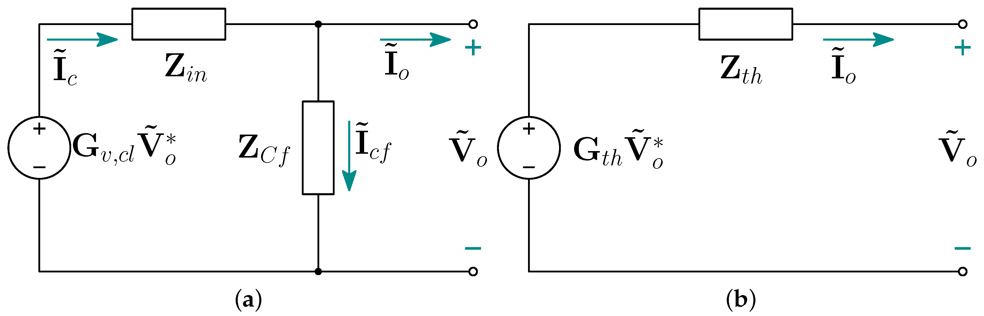
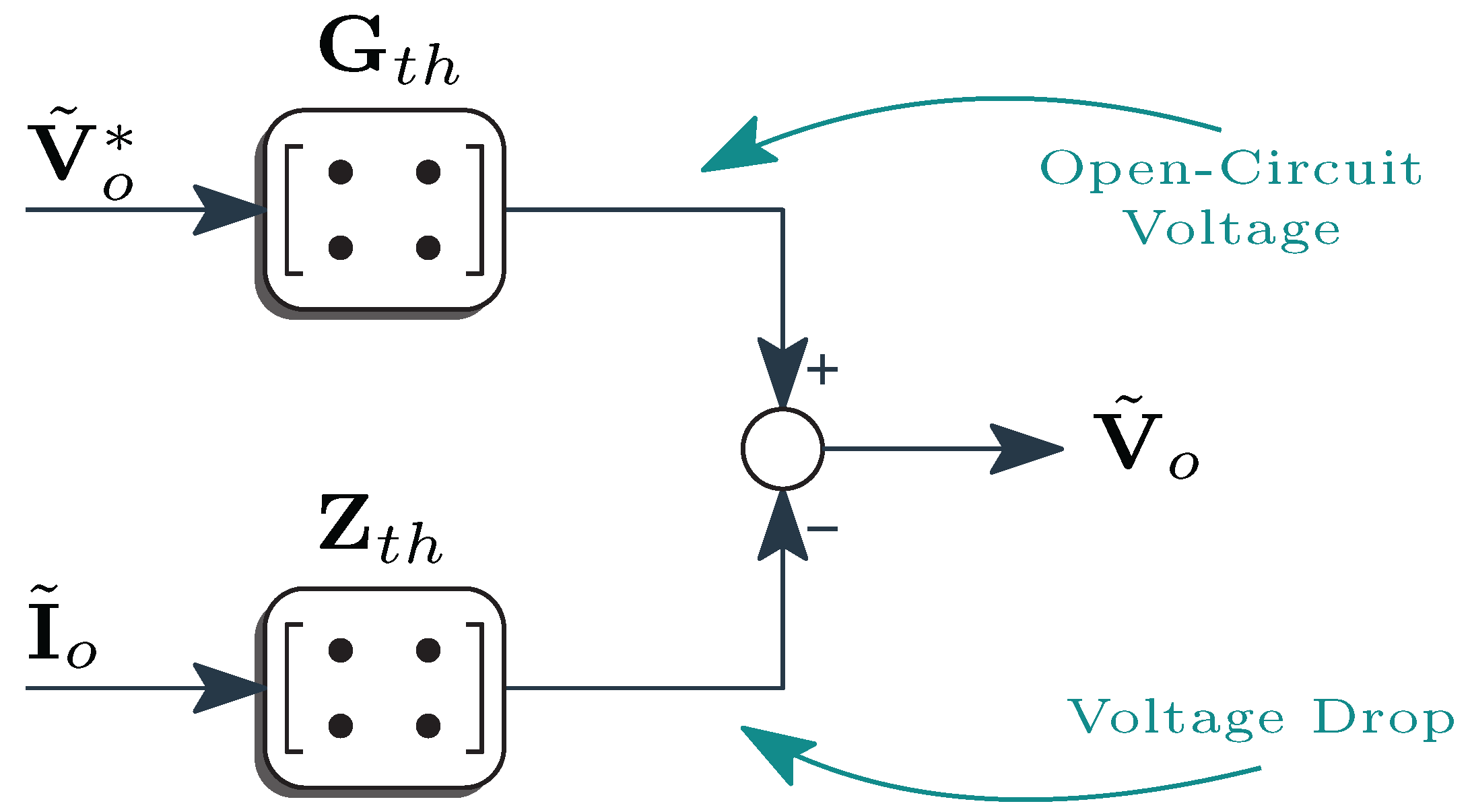
• A small-signal model for a grid-forming MMC with dual-loop control. This model includes not only the equivalent impedance, but also the open-circuit voltage-to-reference transfer matrix of the converter;
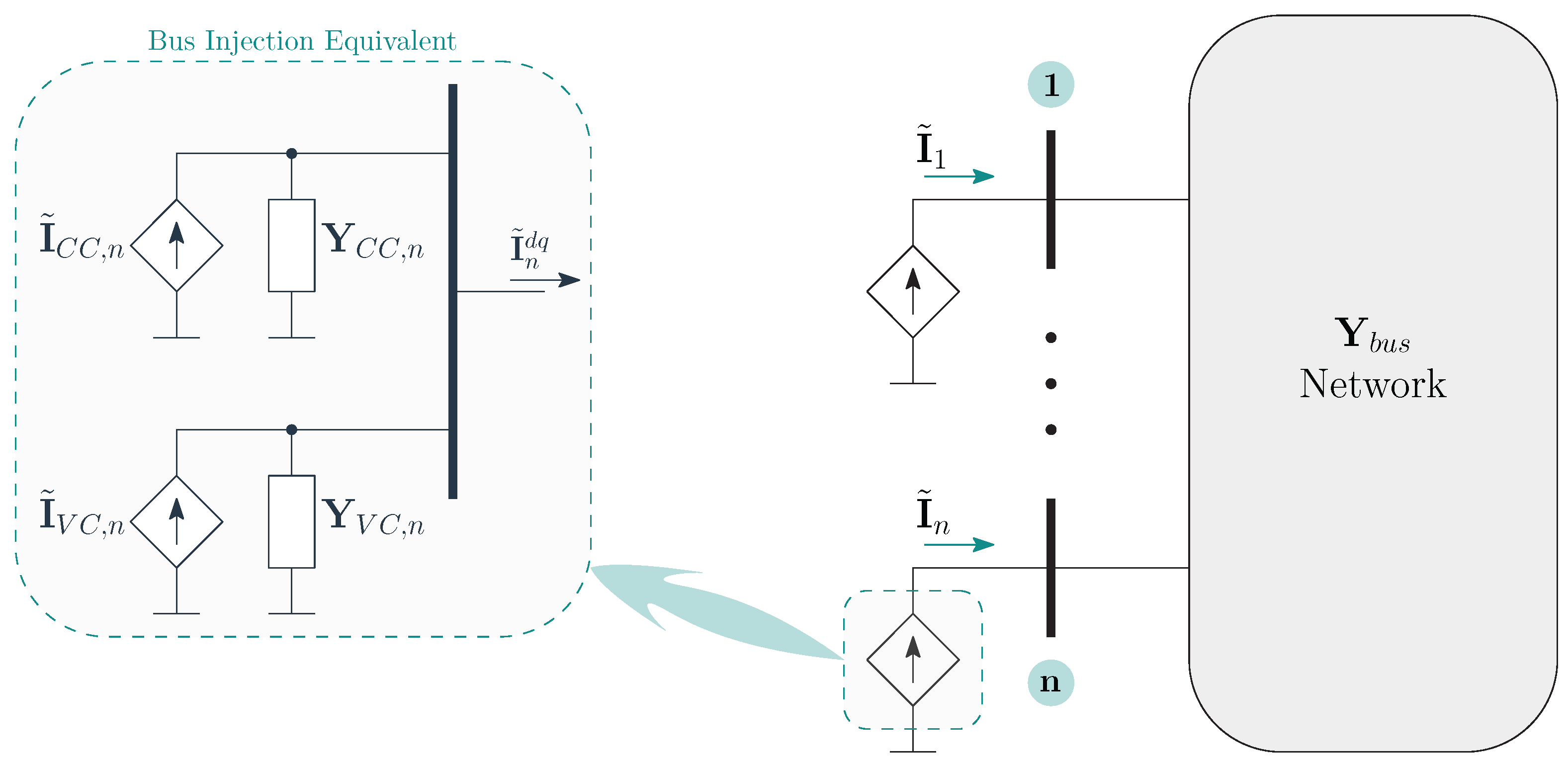
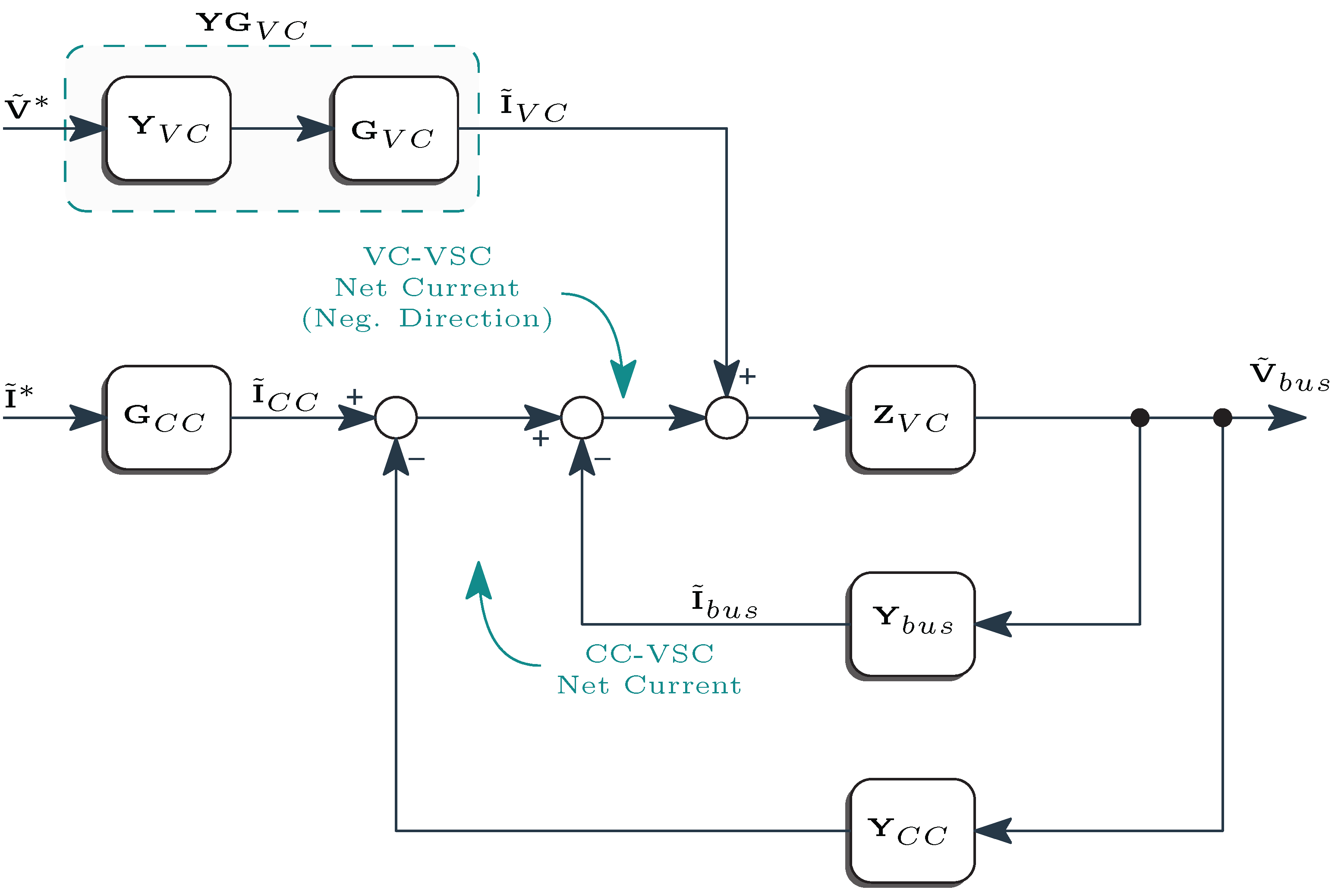
• A framework for simulation and analyzing inverter-based power grids using impedance models and voltage-to-reference and current-to-reference transfer matrices.

This work is divided in six sections, covering the basic concepts of the MMC for the development and validation of the proposed simulation framework. In short, Section 2 presents some basic concepts about the MMC and its time–domain state equations in natural reference frame. In Section 3, firstly, the linearized equations presented in the previous section are transformed into synchronous reference frame (SRF) and then transformed into the Laplace domain. The control loops of the MMC are also presented in this section before the proposed model is developed in detail. Section 4 focuses on validating the proposed model through simulation results. Section 5 presents the proposed simulation framework and its validation. Finally, Section 6 draws the conclusions of this paper.

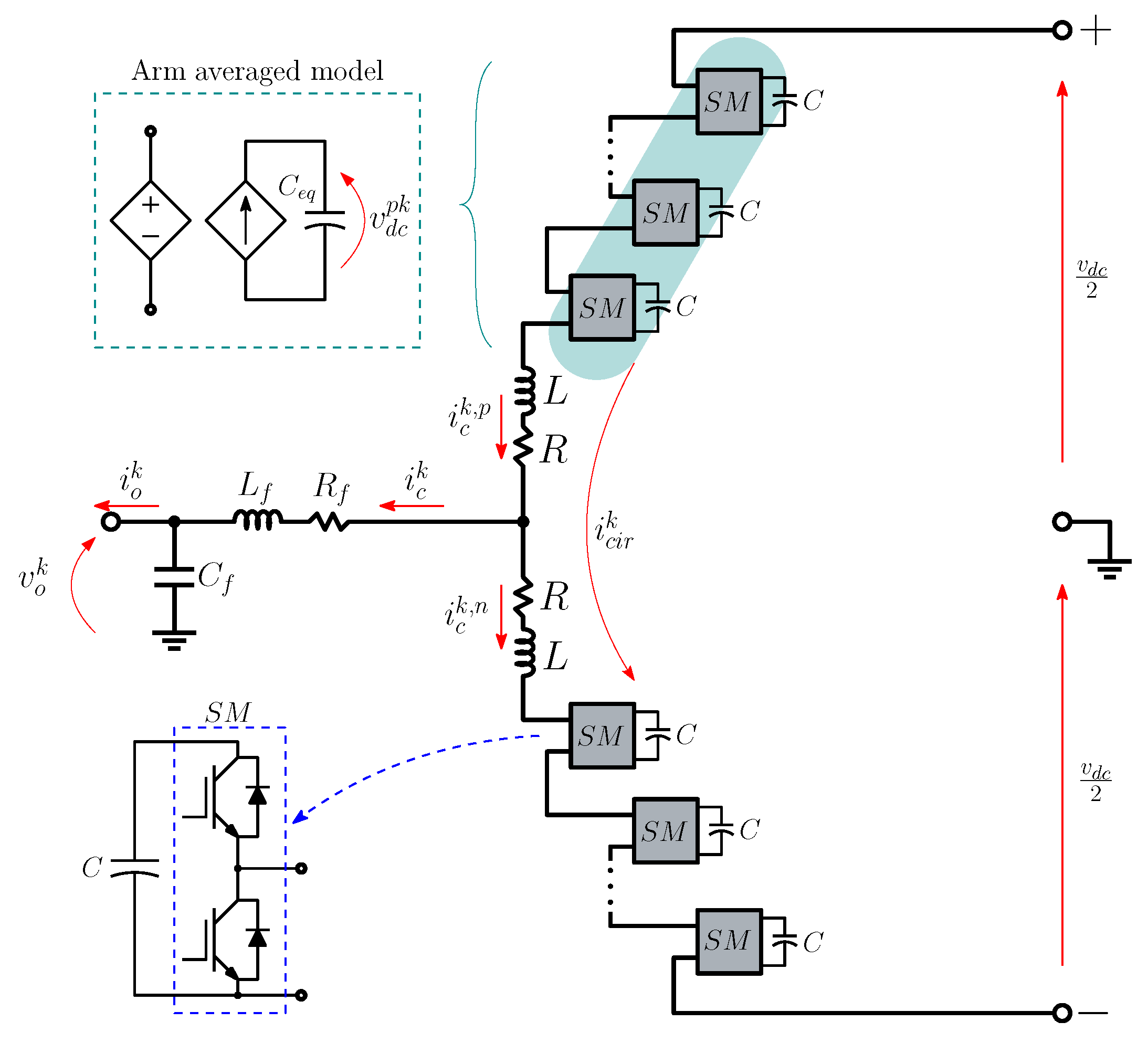
2. Modular Multilevel Converter

Figure 1 depicts the studied MMC. It comprises N half-bridge submodules (SM) in series with LR circuit at both the upper and lower arms of the converter. Moreover, there is a RLC circuit, indicated by $L_f$, $R_f$, and $C_f$, synthesizing a filter between the MMC and the grid. It is important to mention that this RLC net was included to make the results as generic as possible. Thus, during the usage of the model, RL may represent the series-equivalent parameters of a transformer, and $C_f$ may represent the capacitance of a transmission line or even a capacitor bank in the grid. In this article, nonetheless, we assigned generic values for this RLC net, considering them neither as transformers nor as transmission lines.

Back to Figure 1, the notation $x^k$ refers to the variables in natural reference frame (NRF), where $k=a,b,c$ is the phase to which the variable is related. In this case, the AC voltages $v_o^k$ are produced by the MMC, supplied by a dc-voltage source ($v_{dc}$). The currents delivered to the load are represented by $i_o^k$, whereas $i_c^k$ represents the currents produced by the converter.

Still, in Figure 1, the currents flowing through the upper and lower arms of the converter are $i_c^{k,p}$ and $i_c^{k,n}$, respectively. Furthermore, $i_{cir}^k$ denotes the circulating current within the MMC. The insertion indices, as defined by [29], correspond to the number of the inserted SMs. It is defined as follows:

$$m_p^k=\frac{1}{2}\left(1-e_c^{k*}-e_{cir}^{k*}\right);$$

(1)

$$m_n^k=\frac{1}{2}\left(1+e_c^{k*}-e_{cir}^{k*}\right);$$

(2)

where $e_c^{k*}$ are the reference signals to generate the ac voltages, whereas $e_{cir}^{k*}$ are necessary to mitigate the circulating currents.

For purpose of modeling, the upper and lower groups of SMs were represented by their average models, i.e., a pair of linear sources labeled in Figure 1 arm average model. In this case, $v_{}^{p,k}$ and $v_{}^{n,k}$ are the equivalent dc voltages of the upper and lower arms of the phase k, and $C_{eq}=C/N$ is the equivalent capacitance of each arm [30].

According to [21], the small-signal dynamics of the MMC, not including the circulating current, are given by:

$$2C_{eq}\frac{d{\tilde{v}}_{dc}^{k\Delta }}{dt}=-\frac{2S_0}{3V_{dc0}}{\tilde{e}}_c^k+{\tilde{i}}_c^k;$$

(3)

$$2\left(L+2L_f\right)\frac{d{\tilde{i}}_c^k}{dt}=2V_{dc0}{\tilde{e}}_c^{k*}-{\tilde{v}}_{dc}^{k\Delta }-4{\tilde{v}}_o^k-2\left(R+2R_f\right){\tilde{i}}_c^k;$$

(4)

where $S_0$ and $V_{dc0}$ are the produced power and the dc-bus voltage at steady-state condition. The tildes notation in the variables indicate small-signal quantities, with ${\tilde{v}}_{dc}^{k\Delta }$ representing the difference between the upper and lower dc voltages of the MMC, i.e., ${\tilde{v}}_{dc}^{k\Delta }={\tilde{v}}_{dc}^{pk}-{\tilde{v}}_{dc}^{nk}$ [31]. Notice that, different from a two-level converter, the MMC ac model contains the dynamics of the dc capacitors, even when the dc bus is driven by a stiff voltage source $V_{dc}$.

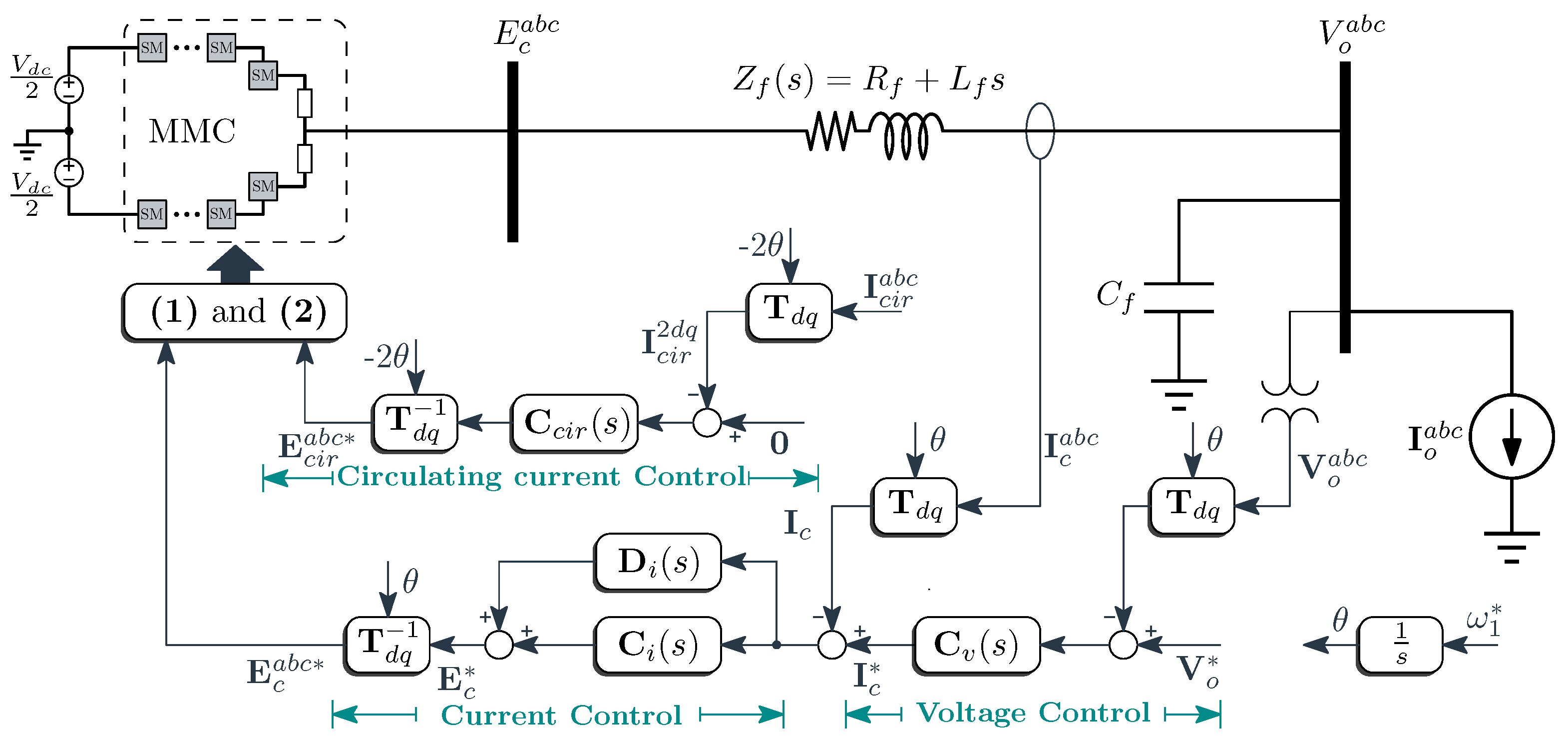
3. Control and Modeling of the MMC

The starting point of the modeling process is to aggregate the submodules (SM) into a pair of equivalent sources, one to the ac side, and another for the dc side. For the lack of space, we chose not to present this process, but more information can be found in our previous papers [21,32].

Figure 2 presents an overall view of the applied control-loops to the MMC. The control system comprehends three control loops: one to mitigate the second-harmonic component of the circulating current. The remaining ones control the converter AC-side, which refers to the output current ($i_c^k$) and the main-bus voltage ($v_o^k$). The outer voltage control loop computes the reference $i_c^{k*}$ for the inner loop so as to drive $v_o^k$ toward the designated reference $v_o^{k*}$. The SRF was chosen for the control loops of the output voltages and currents, whereas the doubly SRF (D-SRF) was used for the circulating-current control to transform the negative-sequence second harmonic components into dc quantities. Still, in Figure 2, notice that ${\mathbf{T}}_{dq}$ and ${\mathbf{T}}_{dq}^{-1}$ represent the Park transformation and its inverse, whereas $\theta$ is the electrical angle. As the work focus on the dynamics of the inner control loops, it was not considered any energy-balancing system for the MMC.

The Vector notation $\mathbf{x}={\left[x_d,x_q\right]}^T$ represents these variables in the synchronous-reference frame quantities. The dq notation was necessary to reduce the size of the equations, enabling their use in matrix algebra, as described hereafter.

3.1. Output-Current Loop

Initially, the small-signal dynamics of the MMC ac-side, already presented in [21,32], are rewritten into SRF as follows:

$$2C_{eq}\left(\mathsf{\Omega }+s\mathbf{I}\right){\tilde{\mathbf{V}}}_{dc}^{\Delta }=-\frac{2S_0}{3V_{dc0}}{\tilde{\mathbf{E}}}_c^{*}+{\tilde{\mathbf{I}}}_c^{},$$

(5)

$$2\left(L+2L_f\right)\left(\mathsf{\Omega }+s\mathbf{I}\right){\tilde{\mathbf{I}}}_c^{}=2V_{dc0}{\tilde{\mathbf{E}}}_c^{*}-{\tilde{\mathbf{V}}}_{dc}^{\Delta }-4{\tilde{\mathbf{V}}}_o^{}-2\left(R+2R_f\right){\tilde{\mathbf{I}}}_c^{},$$

(6)

where each tilde-covered capital letter refers to Laplace-domain vectors, such that $\mathbf{X}={\left[X_d\left(s\right),X_q\left(s\right)\right]}^T$. As for $\mathbf{I}$, it is simply a $2\times 2$ identity matrix to link the complex frequency s with each component. Furthermore, $S_0$ and $V_{dc0}$ are steady-state values of the produced power and dc-bus voltage, representing the point around which the linearization was conducted. Indeed, these values should be chosen in accordance with the operational condition at which the analysis will be conducted. The variables ${\tilde{\mathbf{V}}}_{dc}^{\Delta }$, ${\tilde{\mathbf{E}}}_c^{*}$, and ${\tilde{\mathbf{I}}}_c^{}$ represent the difference voltage between the upper and lower SM dc voltages, the modulation reference, and the output current, respectively.

As a consequence of the frame transformation, a coupling term $\mathsf{\Omega }$ comes out:

$$\mathsf{\Omega }=\left[\begin{array}{cc}0& -{\omega }_1\\ {\omega }_1& 0\end{array}\right],$$

(7)

where ${\omega }_1$ is the angular frequency of the fundamental component. For the sake of simplifying equations, from this point on, the SRF complex frequency (${\mathbf{s}}_{dq}$) denotes the $\mathsf{\Omega }+s\mathbf{I}$ matrix.

As presented in Figure 2, the error between output current, ${\tilde{\mathbf{I}}}_c^{}$, and its reference, ${\tilde{\mathbf{I}}}_c^{*}$, is multiplied by the controller ${\mathbf{C}}_i^{}$ to produce the reference vector ${\tilde{\mathbf{E}}}_c^{*}$, i.e.:

$${\tilde{\mathbf{E}}}_c^{*}={\mathbf{C}}_i^{}\left({\tilde{\mathbf{I}}}_c^{*}-{\tilde{\mathbf{I}}}_c^{}\right)+{\mathbf{D}}_i^{}{\tilde{\mathbf{I}}}_c^{},$$

(8)

where ${\mathbf{C}}_i^{}=C_i\left(s\right)\mathbf{I}$ is a $2\times 2$ transfer matrix, with $C_i\left(s\right)$ representing the transfer function of PI controllers used for direct- and quadrature-axis control. Moreover, the factor ${\mathbf{D}}_i^{}$ is used to decouple the direct and quadrature axis, and it is given by:

$${\mathbf{D}}_i^{}=\frac{L+2L_f}{V_{dc0}}\mathsf{\Omega }.$$

(9)

Combining (5), (6), and (8), it is possible to reach the equation for the current loop of the MMC, i.e.:

$${\tilde{\mathbf{I}}}_c^{}={\mathbf{G}}_{i,cl}^{}{\tilde{\mathbf{I}}}_c^{*}-{\mathbf{Y}}_{ac}^{}{\tilde{\mathbf{V}}}_o^{}.$$

(10)

This result is compatible with a Norton circuit representation of the MMC with its current control loop. The circuit is not presented here due to lack of space. Note that ${\mathbf{G}}_{i,cl}^{}$ and ${\mathbf{Y}}_{ac}^{}$ are matrices containing the closed-loop current gain and output admittance of the converter. They are given by:

$${\mathbf{Y}}_{ac}^{}=8C_{eq}{\mathbf{\Gamma }}_i^{-1}{\mathbf{s}}_{dq},$$

(11)

$${\mathbf{G}}_{i,cl}^{}={\mathbf{\Gamma }}_i^{-1}\left(4C_{eq}{V}_{dc0}{\mathbf{s}}_{dq}+\frac{2S_0}{3V_{dc0}}\mathbf{I}\right){\mathbf{C}}_i^{},$$

(12)

where ${\mathbf{\Gamma }}_i$ corresponds to:

$${\mathbf{\Gamma }}_i=\mathbf{I}+\left(4C_{eq}{V}_{dc0}{\mathbf{s}}_{dq}+\frac{2S_0}{3V_{dc0}}\mathbf{I}\right){\mathbf{C}}_i^{}+4C_{eq}\left(Z+2Z_f\right){\mathbf{s}}_{dq}-\frac{2S_0}{3V_{dc0}}{\mathbf{D}}_i^{},$$

(13)

where $Z=R+Ls$ and $Z_f=R_f+L_{f}s$.

3.2. Main-Bus Voltage Loop

The outer control loop of the ac side aims at controlling the voltage $v_o$ in the main bus, as already mentioned. This voltage control loop receives the reference voltage vector ${\tilde{\mathbf{V}}}_o^{*}$ and computes the reference current, which might drive the voltage toward this value. Thus, according to Figure 2, it is possible to write:

$${\tilde{\mathbf{I}}}_c^{*}={\mathbf{C}}_v^{}\left({\tilde{\mathbf{V}}}_o^{*}-{\tilde{\mathbf{V}}}_o^{}\right).$$

(14)

The voltage controller ${\mathbf{C}}_v^{}=C_v\left(s\right)\mathbf{I}$, similar to the current control-loop, is a diagonal transfer matrix, and $C_v\left(s\right)$ represents the PI transfer functions used in the voltage loop. Substituting (14) in (10) with algebraic manipulations, one may reach the following result:

$${\tilde{\mathbf{V}}}_o^{}={\mathbf{Z}}_{in}^{}{\mathbf{G}}_{i,cl}^{}{\mathbf{C}}_v^{}{\tilde{\mathbf{V}}}_o^{*}-{\mathbf{Z}}_{in}^{}{\tilde{\mathbf{I}}}_c^{},$$

(15)

where:

$${\mathbf{Z}}_{in}^{}={\left({\mathbf{G}}_{i,cl}^{}{\mathbf{C}}_v^{}+{\mathbf{Y}}_{ac}^{}\right)}^{-1}.$$

(16)

Basically, (15) represents a voltage model without accounting the effect of the capacitor bank, $C_f$. As a matter of fact, ${\mathbf{G}}_{v,cl}^{}={\mathbf{Z}}_{in}^{}{\mathbf{G}}_{i,cl}^{}{\mathbf{C}}_v^{}$ is the closed-loop voltage gain, whereas ${\mathbf{Z}}_{in}^{}$ is an inner series impedance of the converter, as depicted in the equivalent circuit of Figure 3a. Notice this circuit representation is valid only when matrix arithmetic is employed. The usual notation of dq circuits, with independent d and q axes, was avoided here to reduce the size of the figure.

From Figure 3a, one may obtain the following node equation:

$${\tilde{\mathbf{I}}}_c^{}={\tilde{\mathbf{I}}}_o^{}+{\tilde{\mathbf{I}}}_{cf}^{},$$

(17)

where ${\tilde{\mathbf{I}}}_{cf}^{}$ is the vector representing the currents in the capacitor $C_f$. Besides that, in SRF, the relationship between currents and voltages in a capacitor is given by:

$$C_f{\mathbf{s}}_{dq}{\tilde{\mathbf{V}}}_o^{}={\tilde{\mathbf{I}}}_{cf}^{}.$$

(18)

Finally, combining (17) and (18) and substituting the result into (15), one may reach the following result:

$${\tilde{\mathbf{V}}}_o^{}={\mathbf{G}}_{th}{\tilde{\mathbf{V}}}_o^{*}-{\mathbf{Z}}_{th}{\tilde{\mathbf{I}}}_o^{}.$$

(19)

It corresponds to the Thévenin-equivalent net equation of the MMC, with both inner ac current control loop and the outer ac voltage loop. Figure 3b depicts this equivalent model. ${\mathbf{G}}_{th}$ is the closed-loop voltage gain, and ${\mathbf{Z}}_{th}$ is the equivalent series impedance of the system. These terms are given by:

$${\mathbf{Z}}_{th}={\left(\mathbf{I}+C_f{\mathbf{Z}}_{in}^{}{\mathbf{s}}_{dq}\right)}^{-1}{\mathbf{Z}}_{in}^{},$$

(20)

$${\mathbf{G}}_{th}={\mathbf{Z}}_{th}{\mathbf{G}}_{i,cl}^{}{\mathbf{C}}_v^{}.$$

(21)

From a transfer-matrix point of view, ${\mathbf{G}}_{th}$ represents a dimensionless voltage gain. It receives the reference voltage of the MMC as an input, and it returns the open-circuit voltage of the converter. As for ${\mathbf{Z}}_{th}$, it clearly represents an impedance, which indicates that it receives the MMC ac current as input and outputs the voltage drop in the circuit. Figure 4 summarizes this information.

One last point should be addressed: as already mentioned, the developed model is valid for small-signal analysis. Thus, it is intended for understanding the dynamics of the MMC whenever a disturbance (load change, for instance) appears in the system. Besides that, the model should be useful, as well, for spotting resonances and helping design control systems. On the other hand, the model is not valid to evaluate the initial transients or the system behavior during faults.

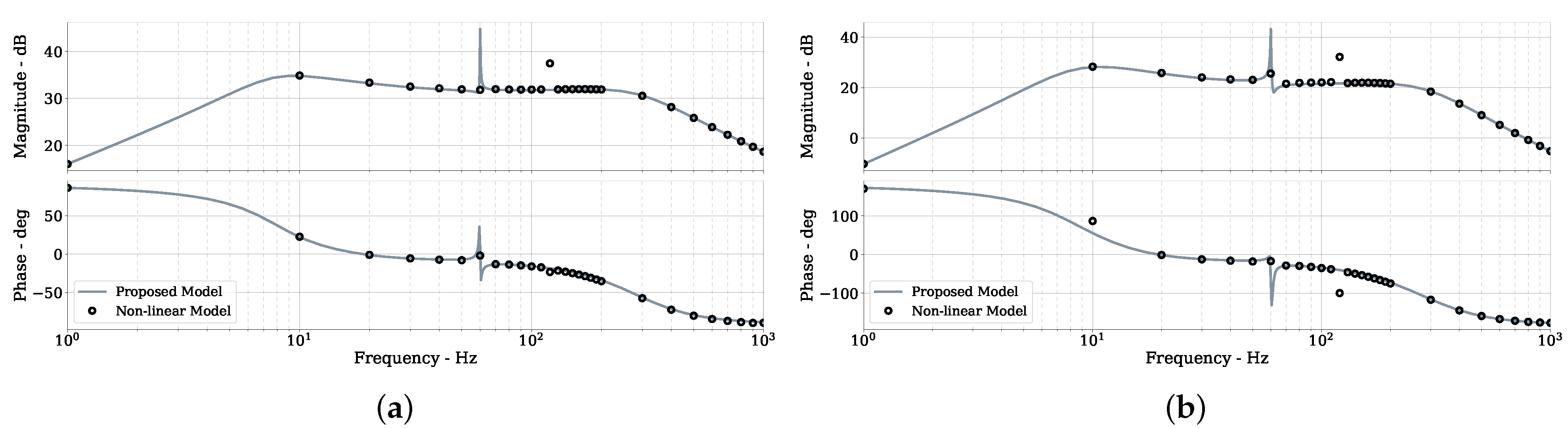
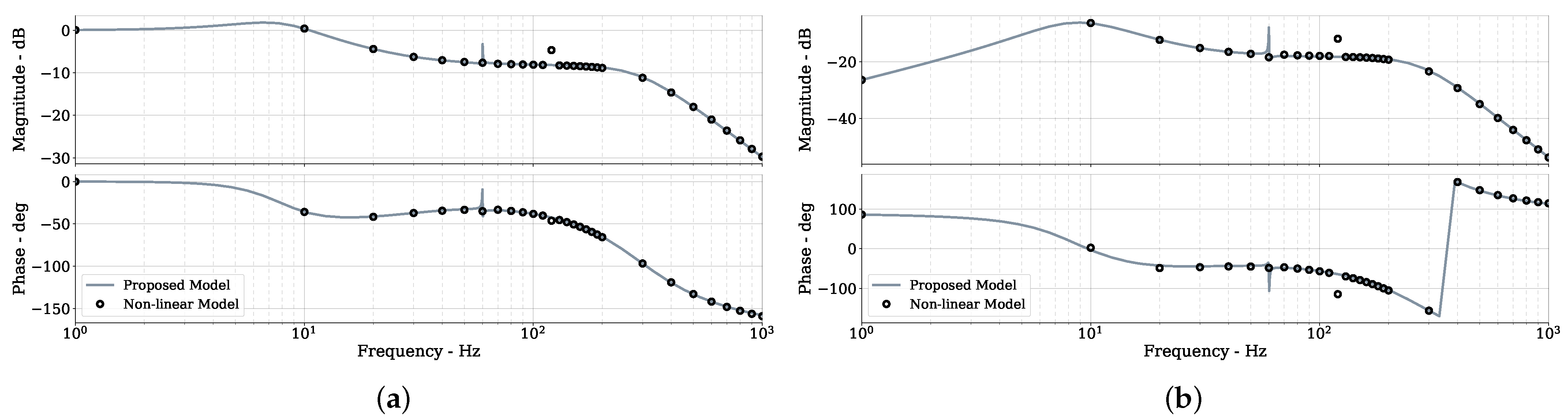
4. Frequency Responses of the MMC

The main objective of this section is to validate the aforementioned transfer functions. Essentially, a time–domain non-linear model of the proposed system was simulated and used as a base for numerically obtaining the system transfer functions. In sequence, there is a comparison between the obtained results through the time–domain model to the ones predicted by the analytic model developed in Section 3. As already mentioned, all of the control loops have PI controllers with their proportional gains and time constants described in

Table A1. Control Gains of the MMC.

MMC
Current-loop Control	$k_p$/$T_i$	0.001 ${\mathrm{A}}^{-1}$/0.01 s
Voltage-loop Control	$k_p$/$T_i$	0.01 ${\mathrm{AV}}^{-1}$/0.01 s
Circ-Current-loop Control	$k_p$/$T_i$	0.001 ${\mathrm{A}}^{-1}$/0.01 s

in the Appendix A. As for the other MMC parameters, they are presented in the

Table A2. Parameters used in MMC.

MMC
Rated Power	-	100 MVA
Rated AC Voltage	-	69 kV
Rated DC Voltage	-	150 kV
Number of SMs	N	20
SM Capacitor	C	9000 $\mathsf{\mu }$F
Arm Impedance	R/L	1 $\Omega$/19 mH
Output Impedance	$R_f$/$L_f$	1 $\Omega$/20 mH
AC capacitor bank	$C_f$	20 $\mathsf{\mu }$F

, as well as in the Appendix A.

The transfer matrices in this section, ${\mathbf{G}}_{th}$ and ${\mathbf{Z}}_{th}$, have the following pattern:

$$\mathbf{M}=\left[\begin{array}{cc}{M}_{dd}& M_{dq}\\ M_{qd}& M_{qq}\end{array}\right],$$

(22)

where the terms $M_{dd}$ and $M_{qq}$ are the d- and q-axis self-related terms, and $M_{dq}$ and $M_{qd}$ are the cross-coupling terms. Due to the symmetry of the system, $M_{dd}=M_{qq}$ and $M_{dq}=-M_{qd}$ [33], are the only frequency responses for two of the terms, ($M_{dd}$ and $M_{dq}$), of each transfer matrix, which are needed to validate the model.

For obtaining ${\mathbf{G}}_{th}$ from the non-linear model, the MMC simulated delivering voltages to a current-source load, as in Figure 2. Then, a sinusoidal disturbance with frequency ${\omega }_p$ was introduced in one of the axis (d or q) of the reference voltage (input), at a time, and the corresponding voltage components ${\mathbf{G}}_{th}\left(j{\omega }_p\right)$ (output) were measured. The closed-loop voltage gain components were computed, then, as follows:

$$\left|G_{th,dd}\left({\omega }_p\right)\right|=\left|\frac{{\tilde{v}}_{o,d}\left({\omega }_p\right)}{{\tilde{v}}_{o,d}^{*}\left({\omega }_p\right)}\right|and\angle G_{th,dd}\left({\omega }_p\right)=arctan\left[\frac{{\tilde{v}}_{o,d}\left({\omega }_p\right)}{{\tilde{v}}_{o,d}^{*}\left({\omega }_p\right)}\right],$$

(23)

$$\left|G_{th,qd}\left({\omega }_p\right)\right|=\left|\frac{{\tilde{v}}_{o,q}\left({\omega }_p\right)}{{\tilde{v}}_{o,d}^{*}\left({\omega }_p\right)}\right|and\angle G_{th,qd}\left({\omega }_p\right)=arctan\left[\frac{{\tilde{v}}_{o,q}\left({\omega }_p\right)}{{\tilde{v}}_{o,d}^{*}\left({\omega }_p\right)}\right].$$

(24)

A similar procedure was conducted to determine the components of ${\mathbf{Z}}_{th}$, yet, in this time, the input perturbation was injected in one of the axis of the current ${\tilde{\mathbf{I}}}_o^{}$. Once more, the output was the voltage components ${\tilde{\mathbf{V}}}_o^{}\left(j{\omega }_p\right)$, and the computations were conducted accordingly to the following formulation:

$$\left|Z_{th,dd}\left({\omega }_p\right)\right|=\left|\frac{{\tilde{v}}_{o,d}\left({\omega }_p\right)}{{\tilde{i}}_{o,d}\left({\omega }_p\right)}\right|and\angle Z_{th,dd}\left({\omega }_p\right)=arctan\left[\frac{{\tilde{v}}_{o,d}\left({\omega }_p\right)}{{\tilde{i}}_{o,d}\left({\omega }_p\right)}\right],$$

(25)

$$\left|Z_{th,qd}\left({\omega }_p\right)\right|=\left|\frac{{\tilde{v}}_{o,q}\left({\omega }_p\right)}{{\tilde{i}}_{o,d}\left({\omega }_p\right)}\right|and\angle Z_{th,qd}\left({\omega }_p\right)=arctan\left[\frac{{\tilde{v}}_{o,q}\left({\omega }_p\right)}{{\tilde{i}}_{o,d}\left({\omega }_p\right)}\right].$$

(26)

Before following this analysis, as the models are in SRF, the frequencies in the upcoming Bode diagrams are not directly related to the natural grid frequencies. For instance, 60 Hz in the graphs is the frequency of the positive sequence 2nd harmonic component [34] (pp. 169–174). In fact, the grid frequency turns to the dc component, which is well known.

Figure 5 presents the frequency responses for the terms of ${\mathbf{Z}}_{th}$, as obtained from the proposed model, as well as the non-linear time–domain simulation (NLTDS). Noticeable differences are clearly visible at 60 and 120 Hz. In short, these differences are due to the linearization process, which cuts off some non-linear characteristics of the MMC. For a better understanding of the effect of the non-linearity at 60 and 120 Hz, notice that the equivalent ac-side voltages produced by the SMs of one arm present both a dc and a 60 Hz component. When the arms are combined, only the 60 Hz appears in the output of the converter.

Now, consider the following d-axis disturbance in the load current at an angular frequency ${\omega }_p$:

$$i_d=I_{p}sin\left({\omega }_{p}t\right).$$

(27)

In the natural reference frame (NRF), the disturbance assumes the following pattern:

$$\left\{\begin{array}{cc}\hfill i_{p,a}& =\frac{I_p}{2}sin\left[({\omega }_p-{\omega }_1)t\right]+\frac{I_p}{2}sin\left[({\omega }_1+{\omega }_p)t\right]\hfill \\ \hfill i_{p,b}& =\frac{I_p}{2}sin\left[({\omega }_p-{\omega }_1)t+2\pi /3\right]+\frac{I_p}{2}sin\left[({\omega }_1+{\omega }_p)t-2\pi /3\right]\hfill \\ \hfill i_{p,c}& =\frac{I_p}{2}sin\left[({\omega }_p-{\omega }_1)t-2\pi /3\right]+\frac{I_p}{2}sin\left[({\omega }_1+{\omega }_p)t+2\pi /3\right]\hfill \end{array}\right.$$

(28)

Notice that the SRF disturbance at 60 Hz produces dc and 120 Hz NRF components in the load current. As for the 120 Hz SRF disturbance, 60 and 180 Hz current components are established in the NRF. The dc component associated with the 60 Hz SRF disturbance goes within the converter, interacts with SM equivalent voltages, and, once these voltages contain dc components as well, results in active power. As a consequence, the dc voltages of the SM capacitors are modified during the test. Similarly, the NRF 60 Hz component associated to the SRF 120 Hz disturbance interacts with its counterpart in SM equivalent ac voltage, results in active power, and changes the dc level of the SM capacitors. In both cases, a SRF disturbance in one frequency (first 60 Hz, and then 120 Hz) of one variable is causing an effect in another frequency (dc component) of another variable (the equivalent dc voltage of the SMs). Of course, this is a non-linear phenomenon not considered in the proposed model. The same issue is not observed with disturbances of any other frequency because, as can be seen in (28), they do not produce harmonic components matching the components of the equivalent ac-side SM voltages.

Figure 6 presents the frequency–domain response for Thévenin-equivalent gain, as obtained from the proposed model and from the NLTDS. The indicated gain at the proposed model differs from the behavior of the non-linear time-domain model only at 60 and 120 Hz. As in the case of the Thévenin impedance, these difference are due to non-linearities that the proposed model does not address. The effect of the non-linearity in the gain is negligible once the difference between the results is only 3.5 dB.

One interesting aspect that should be highlighted is that the presented model is able to represent the MMC in a frequency range that goes from nearly 0 to 1 kHz. This range covers a wide variety of electromagnetic phenomena in power systems. Although it is not the focus of the present article, it is valid to mention that model-order reduction methods can be used for further simplifications in case the end user focuses their analysis on low-frequency phenomena.

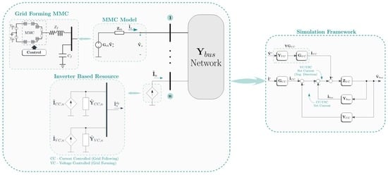
5. Impedance-Based Simulation Framework for Converter-Populated Power Systems

In this section, an impedance-based simulation framework for power-electronics-populated power systems was proposed. The idea was to include the previous MMC results in a model that represents a typical application. Thus, the following subsections detail: (1) the general idea of the proposed framework; (2) the modeling of a 3-bus test case using the framework; and (3) simulation results for the test case.

5.1. Simulation Framework

Figure 7 presents a generic n-bus inverter-based-resource (IBR) power system. It is considered that two converters are connected in each bus, one current-controlled (CC) and another voltage-controlled (VC). As already explained in the introduction, the voltage-controlled converters are in fact grid-forming elements of the grid. This approach of considering two converters per bus will contribute to the modularity of the framework. For now, we need to bear in mind that ${\mathbf{Y}}_{CC,n}$ and ${\mathbf{Y}}_{VC,n}$ are $2\times 2$ matrices, representing the equivalent admittances of the converters, and ${\tilde{\mathbf{I}}}_{CC,n}$ and ${\tilde{\mathbf{I}}}_{VC,n}$ are $2\times 1$ vectors, representing the equivalent currents produced by the converters.

From a system point of view, the injected currents and the bus voltages can be aggregated in single vectors, ${\tilde{\mathbf{I}}}_{bus}$ and ${\tilde{\mathbf{V}}}_{bus}$, as follows:

$${\tilde{\mathbf{I}}}_{bus}={\left[\begin{array}{cccc}{\tilde{\mathbf{I}}}_1& {\tilde{\mathbf{I}}}_2& \cdots & {\tilde{\mathbf{I}}}_n\end{array}\right]}^T,$$

(29)

$${\tilde{\mathbf{V}}}_{bus}={\left[\begin{array}{cccc}{\tilde{\mathbf{V}}}_1& {\tilde{\mathbf{V}}}_2& \cdots & {\tilde{\mathbf{V}}}_n\end{array}\right]}^T.$$

(30)

Then, the system can be represented by the following nodal equation:

$${\mathbf{Y}}_{bus}\left(s\right){\tilde{\mathbf{V}}}_{bus}={\tilde{\mathbf{I}}}_{CC}+{\tilde{\mathbf{I}}}_{VC}-\left[{\mathbf{Y}}_{VC}\left(s\right)+{\mathbf{Y}}_{CC}\left(s\right)\right]{\tilde{\mathbf{V}}}_{bus},$$

(31)

where ${\mathbf{Y}}_{bus}$ is the $n\times n$ bus admittance matrix, and:

$${\mathbf{Y}}_{VC}\left(s\right)=\mathbf{diag}\left({\mathbf{Y}}_{VC,1}^{},{\mathbf{Y}}_{VC,2}^{},\cdots ,{\mathbf{Y}}_{VC,n}^{}\right),$$

(32)

$${\mathbf{Y}}_{CC}\left(s\right)=\mathbf{diag}\left({\mathbf{Y}}_{CC,1}^{},{\mathbf{Y}}_{CC,2}^{},\cdots ,{\mathbf{Y}}_{CC,n}^{}\right),$$

(33)

$${\tilde{\mathbf{I}}}_{VC}={\left[\begin{array}{cccc}{\tilde{\mathbf{I}}}_{VC,1}& {\tilde{\mathbf{I}}}_{VC,2}& \cdots & {\tilde{\mathbf{I}}}_{VC,n}\end{array}\right]}^T,$$

(34)

$${\tilde{\mathbf{I}}}_{CC}={\left[\begin{array}{cccc}{\tilde{\mathbf{I}}}_{CC,1}& {\tilde{\mathbf{I}}}_{CC,2}& \cdots & {\tilde{\mathbf{I}}}_{CC,n}\end{array}\right]}^T,$$

(35)

Given that ${\mathbf{Y}}_{VC}^{-1}={\mathbf{Z}}_{VC}$, the nodal Equation (31) can be rewritten as follows:

$${\tilde{\mathbf{V}}}_{bus}={\mathbf{Z}}_{VC}\left(s\right){\tilde{\mathbf{I}}}_{CC}+{\mathbf{Z}}_{VC}\left(s\right){\tilde{\mathbf{I}}}_{VC}-{\mathbf{Z}}_{VC}\left(s\right)\left[{\mathbf{Y}}_{bus}\left(s\right)+{\mathbf{Y}}_{CC}\left(s\right)\right]{\tilde{\mathbf{V}}}_{bus}.$$

(36)

It is important to notice that currents injected by the current-controlled converters depend on the their closed-loop gains and reference signals, such as expressed here:

$${\tilde{\mathbf{I}}}_{CC}={\mathbf{G}}_{CC}{\tilde{\mathbf{I}}}_{CC}^{*}.$$

(37)

As for the voltage-controlled converters, using the source transformation approach, its injected current can be defined as function of the reference voltage, the closed-loop transfer function, and the equivalent admittance:

$${\tilde{\mathbf{I}}}_{VC}={\mathbf{Y}}_{VC}{\mathbf{G}}_{VC}{\tilde{\mathbf{V}}}_{VC}^{*}.$$

(38)

Equations (36)–(38) can be combined to form the block diagram in the Figure 8. Notice that ${\tilde{\mathbf{Y}}}_{VC}{\tilde{\mathbf{G}}}_{VC}$ will be labeled ${\mathbf{YG}}_{VC}$ for now on to simplify the notation. Besides that, the label CC-VSC net current shows where in the diagram it is possible to obtain the vector with the equivalent currents injected by the current-controlled converters (${\tilde{\mathbf{I}}}_{CC}-{\mathbf{Y}}_{CC}{\tilde{\mathbf{V}}}_{bus}$). Similarly, the label VC-VSC net current indicates the injected currents from the voltage controlled converters. Notice, nonetheless, that, in this case, the arrow presents a negative value, i.e., $-({\tilde{\mathbf{I}}}_{VC}-{\mathbf{Y}}_{VC}{\tilde{\mathbf{V}}}_{bus})$.

The results obtained from the block diagram in Figure 8 correspond to the transient behavior of the system. Thus, the complete response of, for instance, a generic variable $\tilde{\mathbf{X}}\left(t\right)$, it is necessary to make:

$$\mathbf{X}\left(t\right)=\tilde{\mathbf{X}}\left(t\right)+{\mathbf{X}}_{ss}\left(t\right),$$

(39)

where ${\mathbf{X}}_{ss}$ is the steady-state value of $\mathbf{X}$. Notice that ${\mathbf{X}}_{ss}$ can be computed through power flow analysis, yet it was obtained from the switching-level simulations in this work. It is important to mention that the proposed model is valid for perturbations around the steady-state condition, not being intended for large-signal analysis (energizing or fault transients, for instance).

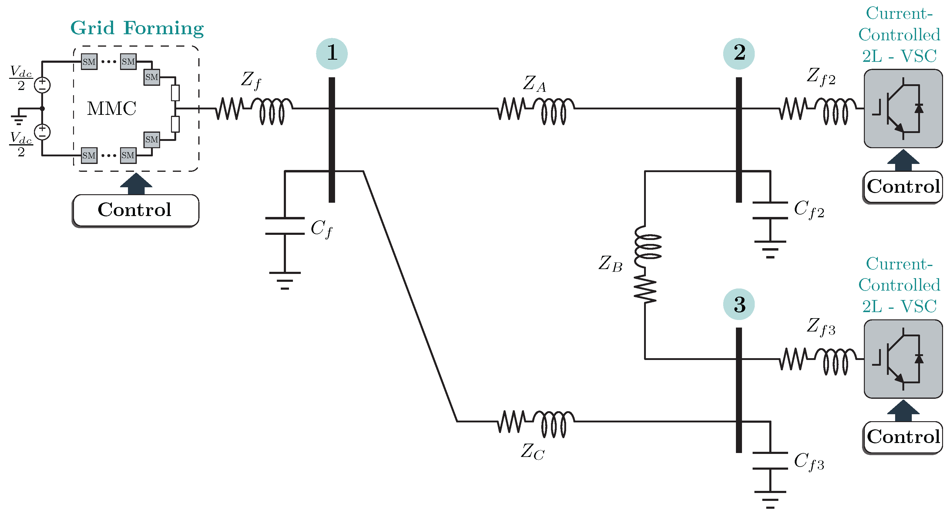
5.2. Three-Bus Test Case

For this test case, a power grid that comprehends a three-bus power system with the voltage-controlled (grid-forming) MMC connected to two grid-following two-level VSCs was considered, as shown in Figure 9. Despite the fact this is a generic system, it contains typical interaction between voltage- and current-controlled VSCs in modern power grids. The following subsection provides a brief description on impedance models for current-controlled VSCs, and the subsequent subsection shows how the matrices of the proposed model should be filled out.

5.2.1. Current-Controlled Two-Level Converter Model

The current-controlled VSCs considered in this work are based on two-level converters (2L-VSC) and modeled as Norton-equivalent circuits. Considering the approach introduced in [35], the 2L-VSCs were expressed based on the Norton representation in the form of:

$${\tilde{\mathbf{I}}}_n^{}={\mathbf{G}}_{2L}\left(s\right){\tilde{\mathbf{I}}}_n^{*}+{\mathbf{Y}}_{2L}\left(s\right){\tilde{\mathbf{V}}}_n^{},$$

(40)

where ${\tilde{\mathbf{V}}}_n$ is the bus voltage, ${\tilde{\mathbf{I}}}_n$ is the current injected in the bus by the VSC, and $n=2,3$, depending on which bus is connected. The matrices ${\mathbf{G}}_{2L}$ and ${\mathbf{Y}}_{2L}\left(s\right)$ represent the closed-loop transfer function and the equivalent admittance of the VSC.

The equivalent admittance is divided into two parts, one representing the inherent characteristic of the current-controlled VSC and another representing the effect of its PLL. Thus:

$${\mathbf{Y}}_{2L}\left(s\right)={\mathbf{Y}}_{PLL}\left(s\right)+{\mathbf{Y}}_{vsc}\left(s\right),$$

(41)

$${\mathbf{Y}}_{vsc}\left(s\right)={\left[{\mathbf{G}}_d{\mathbf{C}}_i+\mathbf{Z}\right]}^{-1},$$

(42)

$${\mathbf{Y}}_{PLL}\left(s\right)=-{\mathbf{Y}}_{vsc}\left(s\right){\mathbf{G}}_d{\mathbf{\Gamma }}_{PLL},$$

(43)

where ${\mathbf{G}}_d$ is the converter transfer function, ${\mathbf{C}}_i$ its current controller, and $\mathbf{Z}$ represents the output RL net.

The term ${\mathbf{\Gamma }}_{PLL}$, on the other hand, corresponds to:

$${\mathbf{\Gamma }}_{PLL}\left(s\right)={\mathbf{G}}_{PLL}^e\left(s\right)+{\mathbf{D}}_i{\mathbf{G}}_{PLL}^i\left(s\right)-{\mathbf{C}}_i\left(s\right){\mathbf{G}}_{PLL}^i\left(s\right),$$

(44)

where ${\mathbf{G}}_{PLL}^e\left(s\right)$ and ${\mathbf{G}}_{PLL}^i\left(s\right)$ are transfer matrices, which are not presented here due to the lack of space. These matrices are found, with the same nomenclature in [35]. Furthermore, the matrix ${\mathbf{D}}_i$ in (44) represents the current decoupling term of the VSC.

Finally, the closed-loop reference-to-current transfer function is given by:

$${\mathbf{G}}_{2L}\left(s\right)={\mathbf{Y}}_{vsc}\left(s\right){\mathbf{G}}_d\left(s\right){\mathbf{C}}_i\left(s\right).$$

(45)

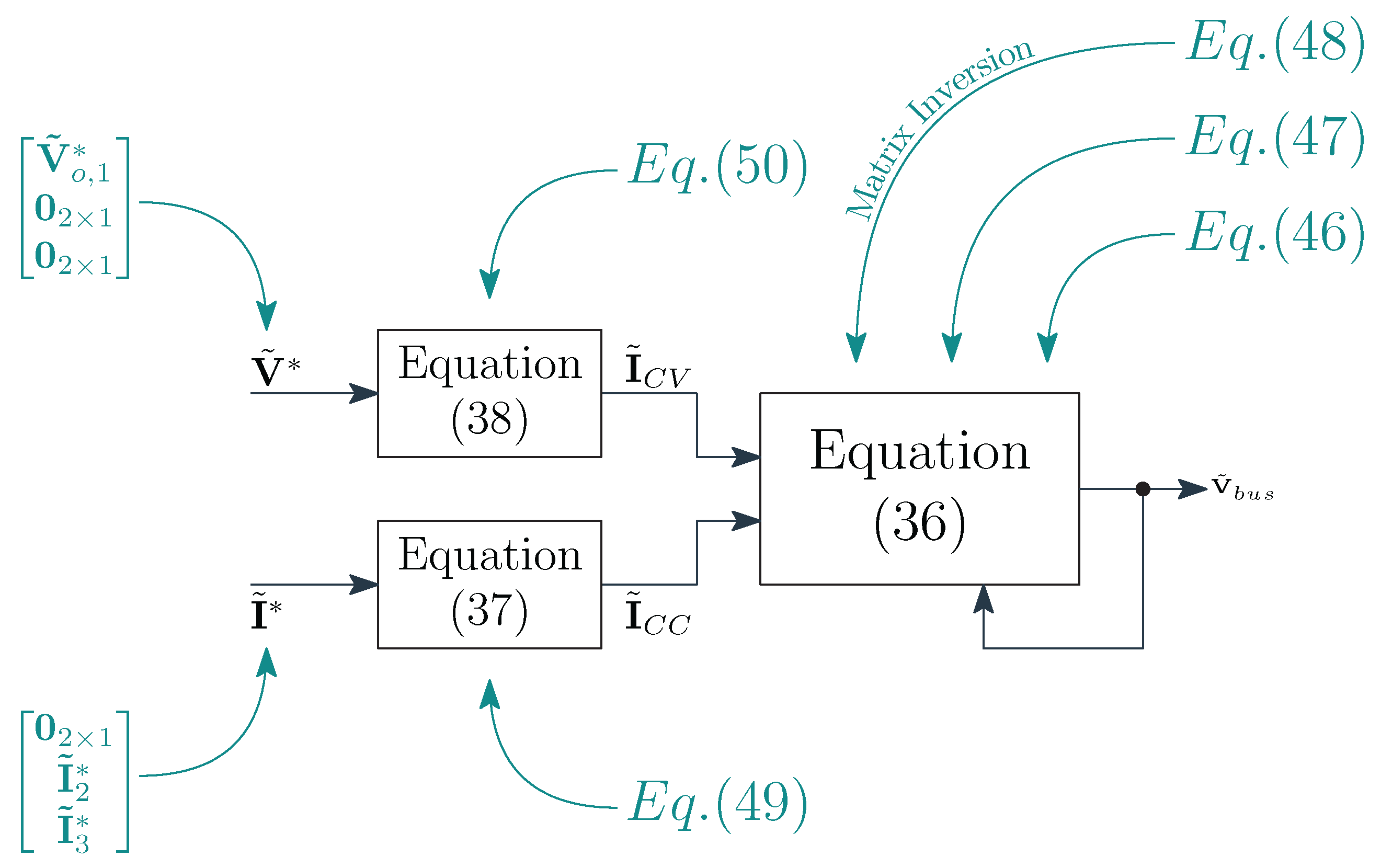
5.2.2. Implementation of the Simulation Framework

Based on the power-grid depicted in Figure 9, the admittance matrix ($Y_{bus}$) corresponds to:

$${\mathbf{Y}}_{bus}\left(s\right)=\left[\begin{array}{ccc}{\mathbf{Y}}_A\left(s\right)+{\mathbf{Y}}_C\left(s\right)& -{\mathbf{Y}}_A\left(s\right)& -{\mathbf{Y}}_C\left(s\right)\\ -{\mathbf{Y}}_A\left(s\right)& {\mathbf{Y}}_A\left(s\right)+{\mathbf{Y}}_B\left(s\right)& -{\mathbf{Y}}_B\left(s\right)\\ -{\mathbf{Y}}_C\left(s\right)& -{\mathbf{Y}}_B\left(s\right)& {\mathbf{Y}}_B\left(s\right)+{\mathbf{Y}}_C\left(s\right)\end{array}\right],$$

(46)

which only comprises the dq admittances linking the three buses of the system. A general representation of these elements are presented in the Appendix B.1. The shunt capacitors (also described in the Appendix B.1), for a decision matter, were included in ${\mathbf{Y}}_{VC}\left(s\right)$ and ${\mathbf{Y}}_{CC}\left(s\right)$. Thus, the output vector ${\mathbf{Y}}_{bus}{\tilde{\mathbf{V}}}_{bus}$ represents the currents flowing through the grid network impedances (${\mathbf{Z}}_A$, ${\mathbf{Z}}_B$, and ${\mathbf{Z}}_C$). ${\mathbf{Y}}_{VC}$ and its inverse, ${\mathbf{Z}}_{VC}$, comprise only the MMC admitance/impedance, as this is the unique voltage-controlled converter in the grid. Nonetheless, to make ${\mathbf{Y}}_{VC}$ non-singular, the empty terms of the main diagonal were represented as negligible matrices, ${\mathbf{Z}}_{\infty }^{-1}$, as follows:

$${\mathbf{Y}}_{VC}\left(s\right)=\mathbf{diag}\left({\mathbf{Z}}_{th}^{-1},{\mathbf{Z}}_{\infty }^{-1},{\mathbf{Z}}_{\infty }^{-1}\right).$$

(47)

A non-singular matrix is necessary, in this case, because the framework takes ${\mathbf{Z}}_{VC}$, which is the inverse of ${\mathbf{Y}}_{GF}$. It is worthwhile mentioning that the inclusion of the terms ${\mathbf{Z}}_{\infty }^{-1}$ in (47) represents the high-valued impedance from buses 2 and 3 to the ground. Thus, the system does not present an significant difference as long as ${\mathbf{Z}}_{\infty }$ remains sufficiently larger than the bus base impedance.

The matrix ${\mathbf{Y}}_{CC}$ for the circuit in Figure 9 is given by:

$${\mathbf{Y}}_{CC}\left(s\right)=\mathbf{diag}\left({\mathbf{0}}_{2\times 2},{\mathbf{Y}}_{2L}+{\mathbf{Y}}_{cf2},{\mathbf{Y}}_{2L}+{\mathbf{Y}}_{cf3}\right),$$

(48)

where ${\mathbf{Y}}_{cf2}$ and ${\mathbf{Y}}_{cf3}$ are the admittance matrices of the capacitor banks connected to buses 2 and 3. Moreover, once there is no current-controlled VSC in bus 1, its place in ${\mathbf{Y}}_{CC}$ was filled with a $2\times 2$ zero matrix, ${\mathbf{0}}_{2\times 2}$.

Finally, the matrices representing the relationship between the references ${\tilde{\mathbf{I}}}^{*}$ and ${\tilde{\mathbf{V}}}^{*}$ can be written as follows:

$${\mathbf{G}}_{CC}\left(s\right)=\mathbf{diag}\left({\mathbf{0}}_{2\times 2},{\mathbf{G}}_{2L},{\mathbf{G}}_{2L}\right),$$

(49)

$${\mathbf{YG}}_{VC}\left(s\right)=\mathbf{diag}\left({\mathbf{Z}}_{th}^{-1}{\mathbf{G}}_{th},{\mathbf{0}}_{2\times 2},{\mathbf{0}}_{2\times 2}\right).$$

(50)

As in ${\mathbf{Y}}_{CC}$, the first term of ${\mathbf{G}}_{CC}$ is filled with a zero matrix due to the lack of current-controlled converters in bus 1. Similarly, as the buses 2 and 3 do not have grid-forming converters, the corresponding terms of ${\mathbf{YG}}_{VC}$ are also filled with zero matrices. It is important to remember that the expressions described in the current subsection are entries of the block diagram in Figure 8. For a faster understanding the relationships between the different equations, we provided the diagram in Figure A1 in Appendix B.3. Also, we provided a summary of equations in form of table in the Appendix B.2.

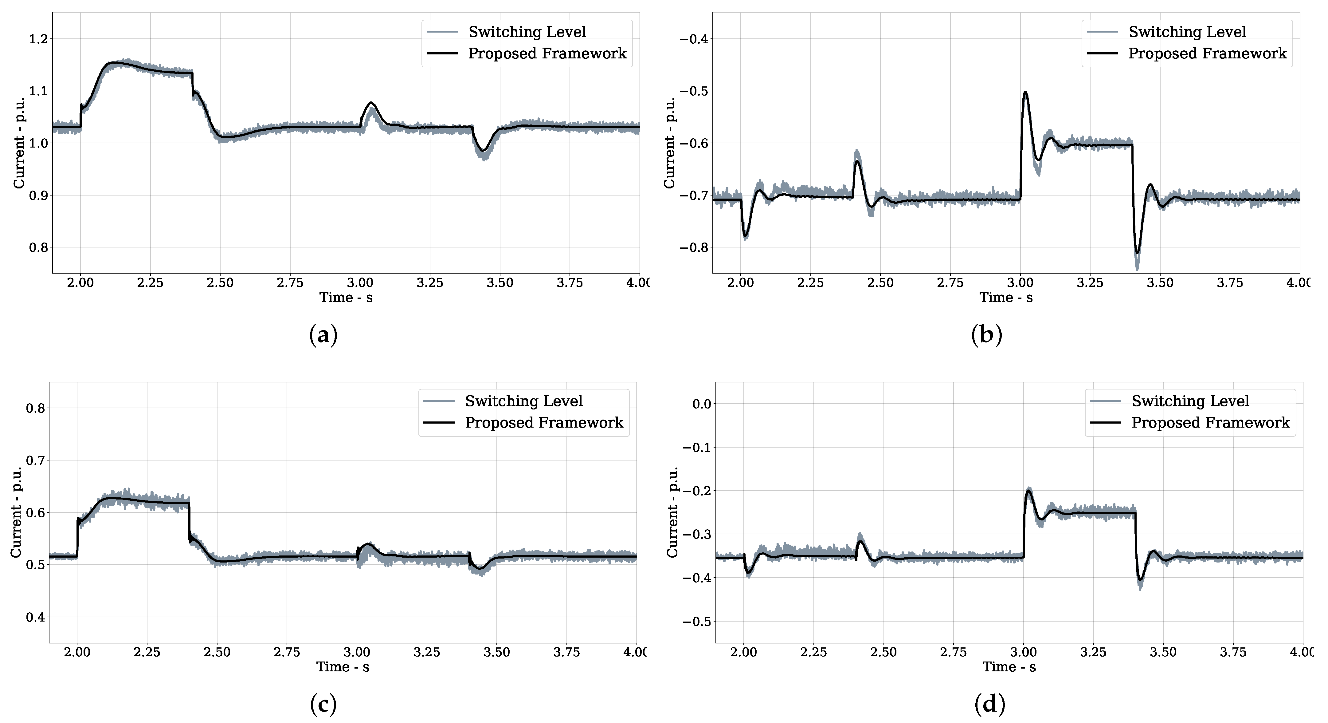
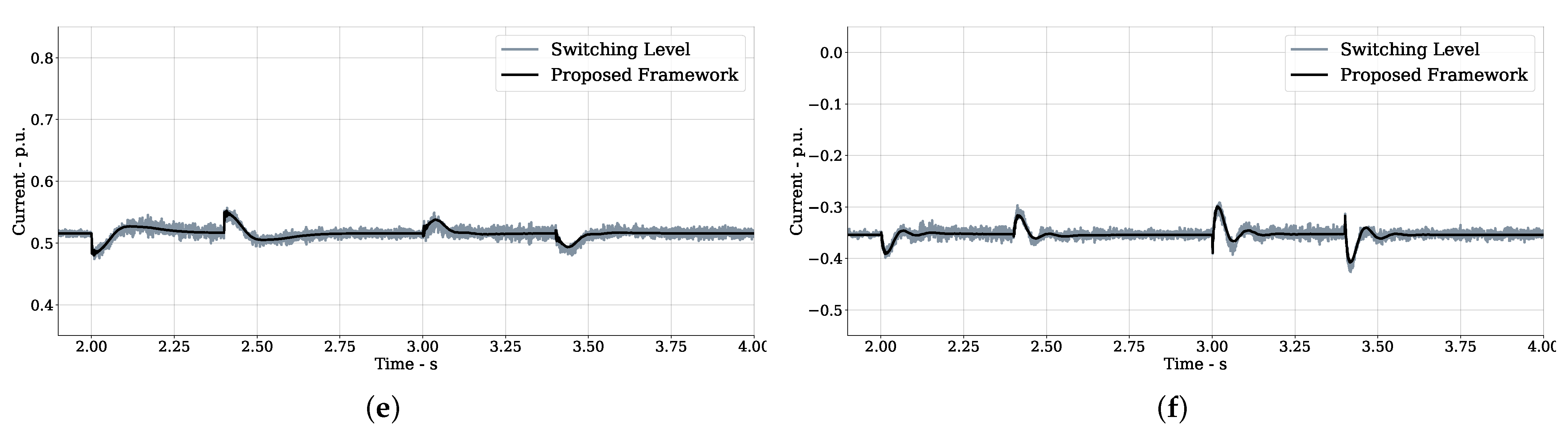
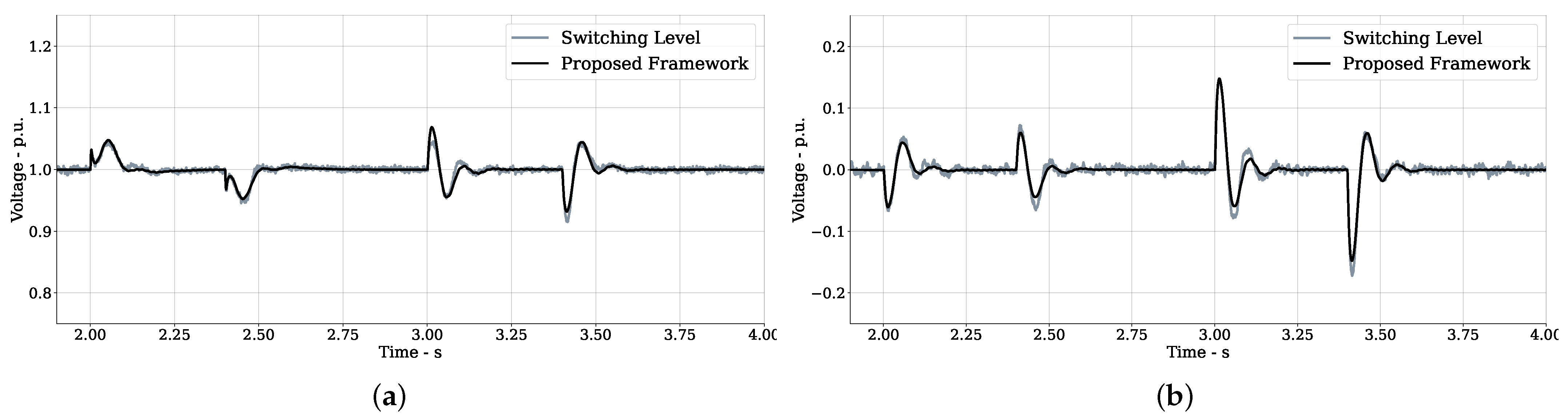
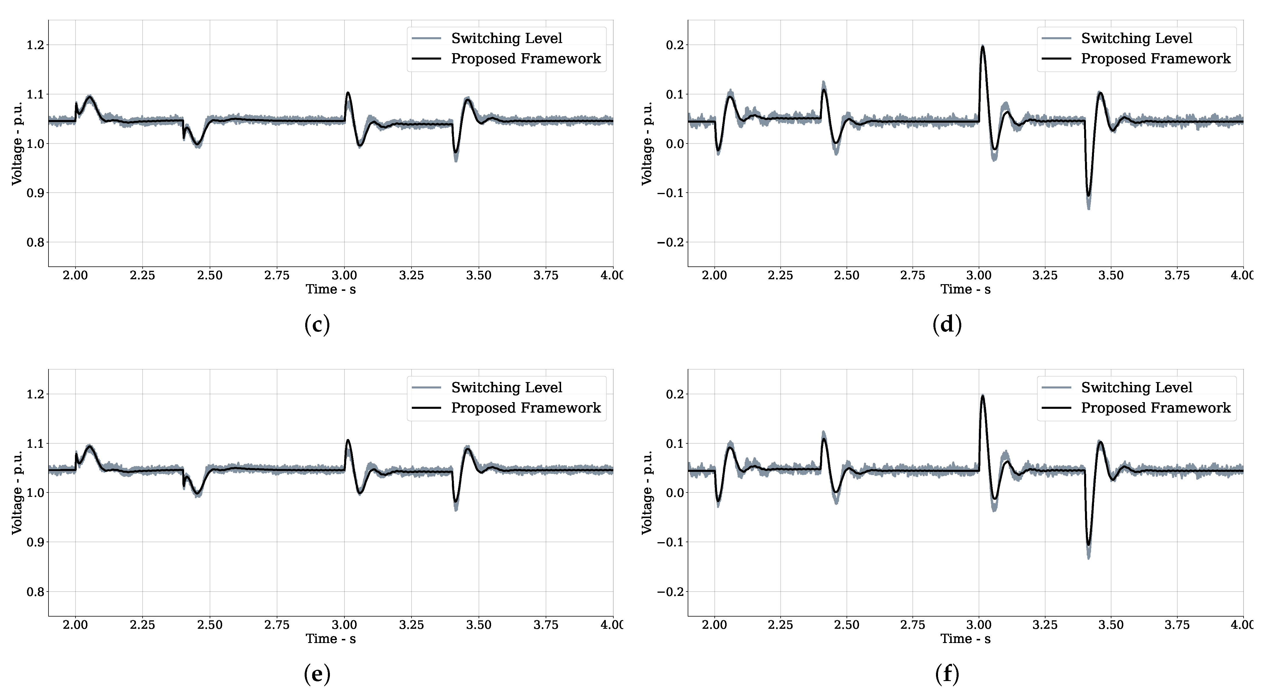
5.3. Results and Comparison

For validating the proposed simulation framework, its time–domain results were compared to the ones obtained from a switching-level simulation in EMTDC/PSCAD. Differently from the non-linear model used for validation in Section 4, the PSCAD model of the MMC comprises each of the submodules, the phase disposition PWM (PD-PWM) modulator, and the dc-voltage-balancing system, (Chapter 2 in [34]). As for the control system, it follows exactly the description introduced in Figure 2. The current-controlled VSCs are based on a two-level topology, following the same premise of previous subsections. Their PSCAD models comprise a 2 kHz PWM modulator, a q-PLL [36] circuit to sync them to their respective bus voltage, and an ac-current control loop.

Table A3. Parameters used in the simulations.

Two-Level VSCs (Reflected to the High-Voltage Side) and Power Grid
Rated Power	-	50 MVA
Rated AC Voltage	-	69 kV
Rated DC Voltage	-	125 kV
Switching Frequency	-	2 kHz
Output Impedance	$R_f$/$L_f$	1 $\Omega$/20 mH
Capacitor bank	$C_{f2}$/$C_{f3}$	20 $\mathsf{\mu }$F
Current-loop Control	$k_p$/$T_i$	0.001 A−1/ 0.1 s
PLL Control	$k_p$/$T_i$	0.1 rad s−1 V−1/0.001 s
Series Impedance A	$R_A$/$L_A$	0.94 $\Omega$/12.5 mH
Series Impedance B	$R_B$/$L_B$	0.94 $\Omega$/12.5 mH
Series Impedance C	$R_C$/$L_C$	0.94 $\Omega$/12.5 mH
Rated Frequency	$f_1$	60 Hz

in the Appendix A summarizes the applied elements in simulations. It is important to notice that, in a real-world application, the 2L-VSCs are connected to the grid through step-up transformers. We decided to omit these transformers for simplifying the mathematical development. Thus, the 2L-VSC parameters in Table A3 are reflected values to the high-voltage side. The MMC settings remains the values indicated in Table A1. The proposed framework was implemented in the Open Modelica [37], an open-source alternative to SIMULINK.

For the intended analysis, the system in Figure 9 was initially in steady-state condition, with the two current-controlled VSCs injecting rated power in their respective buses. As for the MMC, it is also produces a rated voltage in bus 1. From this condition, 0.2 pu pulse disturbances were applied to the reference signals ${\tilde{\mathbf{I}}}_2^{dq*}$, first in the d axis in $2.0\mathrm{s}<t<2.4\mathrm{s}$, then in the q axis in $3.0\mathrm{s}<t<3.4\mathrm{s}$. Figure 10 shows the injected currents by each one of the converters in the grid, i.e., the CC- and CV-VSC net currents in the block diagram of the Figure 8. For this and the next graphs, the black lines represent simulation results obtained with the proposed model, and the gray smudgy curves are from the switching-level PSCAD model. It is important to notice that the smudging pattern in the PSCAD results is due to switching-frequency harmonic components. Notice that the step change in the reference current of the bus 2 VSC produces a slightly underdamped response, as seen in Figure 10c,d. These currents are flowing towards bus 1, where the grid-forming converter is connected. Consequently, a similar pattern is observed in the currents of Figure 10a,b. During the transient, nonetheless, the voltage drops on the impedances of the system disturb all the bus voltages. Thus, small fluctuations appear in the currents of all converters. This phenomenon, correctly predicted by the proposed model, is clearly noticed in the currents of the VSC in bus 3, as shown in Figure 10e,f. Even though its reference current was not changed, there were transient oscillations in their produced currents.

Figure 11 presents the bus voltages when the disturbances were applied. It is noticeable that the proposed simulation framework can capture the electromagnetic transient behavior present in the PSCAD model. For instance, when the d-axis disturbance occurs at $t=2\mathrm{s}$, the corresponding voltages in Figure 11a,c,e swell due to the increase in the energy injected by the VSC in bus 2. The grid-forming MMC reacts to this sudden change, and after 250 ms the bus 1 voltage is stabilized back in 1 pu. The opposite situation occurs when the disturbance is cleaned at $t=2.4\mathrm{s}$. In this case, the VSC in bus 2 reduces the injected current, reducing the injected energy, causing a sudden drop in the d-axis voltages. Once again, after a 250 ms transient, the MMC restores the voltage level at bus 1 to 1 pu. It is important to notice that the transient oscillations observed in all bus voltages are not only due to the response of the grid-forming converter, but also from the voltage drops across the impedances of the system and the interaction of the VSC impedances with the grid. Notice also that, despite the fact the steps in the d and q axes of the reference current of the VSC 2 were equal, the transient behavior was less damped in the q axis. Let us consider, for instance, the voltages in bus 3 in Figure 11e,f. During the d-axis step at 2 s, its transient response endured 125 ms with a 0.1-pu peak-to-peak amplitude. During the q-axis step at 3 s, on the other hand, the transient response spanned over 200 ms, and reached a 0.2-pu peak-to-peak amplitude. A similar pattern difference is observed between the d- and q-axis currents in Figure 10. The origin of both differences is traced back to the interaction between the CC-VSC admittances with the grid. Indeed, these admittances present an asymmetric pattern introduced by the PLLs, causing the axes asymmetry observed in Figure 10 and Figure 11.

6. Conclusions

This paper presented a linearized SRF model for the MMC under a dual-control loop, i.e., with an outer voltage control loop combined with an inner current control loop. The impedance-modeling approach was used, initially for providing the Norton representation of the inner current loop, and then for deriving the Thévenin-equivalent representation of the grid-forming MMC. The validation results, presented in the form of Bode diagrams, showed that the developed model matched accurately the characteristic observed in the non-linear model of MMC. As a matter of fact, the linear model was not able to match its non-linear counterpart in two frequencies, 60 and 120 Hz, both measured in the SRF. When viewed from the natural reference frame, the 60 Hz SRF component encompasses a dc parcel. Similarly, when viewed from the natural reference frame, the 120 Hz SRF component contains a 60 Hz component. These components (dc and 60 Hz) interact with the ac-side arm voltages (that also contain dc and 60 Hz NRF components), producing real power and disturbing the dc-side voltages. This kind of interaction cannot be addressed by a model based on standard linearization. In hypotheses, a harmonic linearization, i.e., a linearization conducted around oscillating trajectories, shall solve this problem. This is going to be pursued in future research.

It is worthwhile to highlight that this model is particularly interesting to analyze the electromagnetic dynamics of grid-forming MMC-based power systems. For this reason, the second half of the paper leaned on proposing a simulation framework for power-electronic-populated grids. In this case, the converters and other elements of the grid are represented in the simulation by their respective impedance matrices. For testing the proposed framework, a three-bus power grid was used. In this case, the MMC supplied the voltages for two current-controlled converters. The obtained results from the proposed simulation framework matched the switching-level EMTDC/PSCAD counterpart.

Moreover, the proposed model for the MMC and the simulation framework should also be used in future researches for evaluating the behavior of the MMC with outer control loops for implementing droop and virtual inertia capabilities.

References

1. Singh, M.; Lopes, L.A.; Ninad, N.A. Grid-forming Battery Energy Storage System (BESS) for a highly unbalanced hybrid mini-grid. Electr. Power Syst. Res. 2015, 127, 126–133. [Google Scholar] [CrossRef]
2. Antonio de Souza Ribeiro, L.; Freijedo, F.D.; de Bosio, F.; Soares Lima, M.; Guerrero, J.M.; Pastorelli, M. Full Discrete Modeling, Controller Design, and Sensitivity Analysis for High-Performance Grid-Forming Converters in Islanded Microgrids. IEEE Trans. Ind. Appl. 2018, 54, 6267–6278. [Google Scholar] [CrossRef] [Green Version]
3. Rodrigues, S.; Restrepo, C.; Kontos, E.; Pinto, R.T.; Bauer, P. Trends of offshore wind projects. Renew. Sustain. Energy Rev. 2015, 49, 1114–1135. [Google Scholar] [CrossRef]
4. Ryndzionek, R.; Sienkiewicz, L. Evolution of the HVDC Link Connecting Offshore Wind Farms to Onshore Power Systems. Energies 2020, 13, 1914. [Google Scholar] [CrossRef] [Green Version]
5. Musca, R.; Vasile, A.; Zizzo, G. Grid-forming converters. A critical review of pilot projects and demonstrators. Renew. Sustain. Energy Rev. 2022, 165, 112551. [Google Scholar] [CrossRef]
6. Lima, L.A.M.; Watanabe, E.H. Hybrid Control Scheme for VSC Presenting Both Grid-Forming and Grid-Following Capabilities. IEEE Trans. Power Deliv. 2022, 37, 4570–4581. [Google Scholar] [CrossRef]
7. Mehrasa, M.; Pouresmaeil, E.; Zabihi, S.; Catalão, J.P.S. Dynamic Model, Control and Stability Analysis of MMC in HVDC Transmission Systems. IEEE Trans. Power Deliv. 2017, 32, 1471–1482. [Google Scholar] [CrossRef]
8. Leon, A.E.; Amodeo, S.J. Modeling, control, and reduced-order representation of modular multilevel converters. Electr. Power Syst. Res. 2018, 163, 196–210. [Google Scholar] [CrossRef]
9. Hao, Q.; Li, Z.; Gao, F.; Zhang, J. Reduced-Order Small-Signal Models of Modular Multilevel Converter and MMC-Based HVdc Grid. IEEE Trans. Ind. Electr. 2019, 66, 2257–2268. [Google Scholar] [CrossRef]
10. Wang, G.; Xiao, H.; Xiao, L.; Zhang, Z.; Xu, Z. Electromechanical Transient Modeling and Control Strategy of Decentralized Hybrid HVDC Systems. Energies 2019, 12, 2856. [Google Scholar] [CrossRef] [Green Version]
11. Stepanov, A.; Mahseredjian, J.; Karaagac, U.; Saad, H. Adaptive Modular Multilevel Converter Model for Electromagnetic Transient Simulations. IEEE Trans. Power Deliv. 2021, 36, 803–813. [Google Scholar] [CrossRef]
12. Hao, Q.; Li, Z.; Yue, C.; Gao, F.; Wang, S. Small-signal Model and Dynamics of MMC- HVDC Grid under Unbalanced Grid Conditions. IEEE Trans. Power Deliv. 2020, 36, 3172–3184. [Google Scholar] [CrossRef]
13. Liu, Z.; Miao, S.; Fan, Z.; Kang, Y.; Tu, Q. Analysis of the performance characteristics and arm current control for modular multilevel converter with asymmetric arm parameters. Int. J. Electr. Power Energy Syst. 2019, 110, 258–270. [Google Scholar] [CrossRef]
14. Wang, J.; Gao, S.; Ji, Z.; Sun, Y.; Hong, L.; Luo, F.; Gu, W. Time/frequency domain modelling for grid-connected MMC sub-synchronous/super-synchronous oscillation in PV MVDC power collection and integration system. IET Renew. Power Gener. 2019, 13, 57–66. [Google Scholar] [CrossRef]
15. Ma, Y.; Lin, H.; Wang, Z. Equivalent Model of Modular Multilevel Converter Considering Capacitor Voltage Ripples. IEEE Trans. Power Deliv. 2019, 34, 2182–2193. [Google Scholar] [CrossRef]
16. Bessegato, L.; Ilves, K.; Harnefors, L.; Norrga, S. Effects of Control on the AC-Side Admittance of a Modular Multilevel Converter. IEEE Trans. Power Electr. 2019, 34, 7206–7220. [Google Scholar] [CrossRef] [Green Version]
17. Man, J.; Xie, X.; Xu, S.; Zou, C.; Yin, C. Frequency-Coupling Impedance Model Based Analysis of a High-Frequency Resonance Incident in an Actual MMC-HVDC System. IEEE Trans. Power Deliv. 2020, 35, 2963–2971. [Google Scholar] [CrossRef]
18. Zhu, S.; Liu, K.; Liao, X.; Qin, L.; Huai, Q.; Xu, Y.; Li, Y.; Wang, F. D-Q Frame Impedance Modeling of Modular Multilevel Converter and Its Application in High-Frequency Resonance Analysis. IEEE Trans. Power Deliv. 2021, 36, 1517–1530. [Google Scholar] [CrossRef]
19. Lyu, J.; Cai, X.; Molinas, M. Frequency Domain Stability Analysis of MMC-Based HVdc for Wind Farm Integration. IEEE J. Emerg. Sel. Top. Power Electron. 2016, 4, 141–151. [Google Scholar] [CrossRef] [Green Version]
20. Sánchez-Sánchez, E.; Prieto-Araujo, E.; Gomis-Bellmunt, O. The Role of the Internal Energy in MMCs Operating in Grid-Forming Mode. IEEE J. Emerg. Sel. Top. Power Electron. 2019, 8, 949–962. [Google Scholar] [CrossRef]
21. Freitas, C.M.; Watanabe, E.H.; Monteiro, L.F.C. A linearized small-signal Thévenin-equivalent model of a voltage-controlled modular multilevel converter. Electr. Power Syst. Res. 2020, 182, 106231. [Google Scholar] [CrossRef]
22. Sun, J.; Liu, H. Sequence Impedance Modeling of Modular Multilevel Converters. IEEE J. Emerg. Sel. Top. Power Electron. 2017, 5, 1427–1443. [Google Scholar] [CrossRef]
23. Beza, M.; Bongiorno, M.; Stamatiou, G. Analytical Derivation of the AC-Side Input Admittance of a Modular Multilevel Converter With Open- and Closed-Loop Control Strategies. IEEE Trans. Power Deliv. 2018, 33, 248–256. [Google Scholar] [CrossRef]
24. Lekić, A.; Beerten, J. Generalized multiport representation of power systems using ABCD parameters for harmonic stability analysis. Electr. Power Syst. Res. 2020, 189, 106658. [Google Scholar] [CrossRef]
25. Li, Y.; Shuai, Z.; Liu, X.; Chen, Y.; Li, Z.; Hong, Y.; Shen, Z.J. Stability Analysis and Location Optimization Method for Multiconverter Power Systems Based on Nodal Admittance Matrix. IEEE J. Emerg. Sel. Top. Power Electron. 2021, 9, 529–538. [Google Scholar] [CrossRef]
26. Liu, H.; Xie, X.; Liu, W. An Oscillatory Stability Criterion Based on the Unified dq-Frame Impedance Network Model for Power Systems With High-Penetration Renewables. IEEE Trans. Power Syst. 2018, 33, 3472–3485. [Google Scholar] [CrossRef]
27. Orellana, L.; Sainz, L.; Prieto-Araujo, E.; Gomis-Bellmunt, O. Stability Assessment for Multi-Infeed Grid-Connected VSCs Modeled in the Admittance Matrix Form. IEEE Trans. Circuits Syst. Regul. Pap. 2021, 68, 3758–3771. [Google Scholar] [CrossRef]
28. Xu, W.; Huang, Z.; Cui, Y.; Wang, H. Harmonic resonance mode analysis. IEEE Trans. Power Deliv. 2005, 20, 1182–1190. [Google Scholar] [CrossRef]
29. Angquist, L.; Antonopoulos, A.; Siemaszko, D.; Ilves, K.; Vasiladiotis, M.; Nee, H. Open-Loop Control of Modular Multilevel Converters Using Estimation of Stored Energy. IEEE Trans. Ind. Appl. 2011, 47, 2516–2524. [Google Scholar] [CrossRef]
30. Ludois, D.C.; Venkataramanan, G. Simplified Terminal Behavioral Model for a Modular Multilevel Converter. IEEE Trans. Power Electron. 2014, 29, 1622–1631. [Google Scholar] [CrossRef]
31. Harnefors, L.; Antonopoulos, A.; Norrga, S.; Angquist, L.; Nee, H. Dynamic Analysis of Modular Multilevel Converters. IEEE Trans. Ind. Electron. 2013, 60, 2526–2537. [Google Scholar] [CrossRef]
32. Freitas, C.M.; Watanabe, E.H.; Monteiro, L.F.C. Grid-Forming MMC: A Comparison Between Single—and Dual-Loop Control Approaches. In Proceedings of the 2021 Brazilian Power Electronics Conference (COBEP), Joao Pessoa, Brazil, 7–10 November 2021; pp. 1–6. [Google Scholar] [CrossRef]
33. Wang, X.; Harnefors, L.; Blaabjerg, F. Unified Impedance Model of Grid-Connected Voltage-Source Converters. IEEE Trans. Power Electron. 2018, 33, 1775–1787. [Google Scholar] [CrossRef] [Green Version]
34. Freitas, C.M. Equivalent Linearized Analytical Models For The Modular Multilevel Converter. Ph.D. Thesis, Federal University of Rio de Janeiro/COPPE, Rio de Janeiro, Brazil, 2020. [Google Scholar]
35. Wen, B.; Boroyevich, D.; Burgos, R.; Mattavelli, P.; Shen, Z. Analysis of D-Q Small-Signal Impedance of Grid-Tied Inverters. IEEE Trans. Power Electron. 2016, 31, 675–687. [Google Scholar] [CrossRef]
36. Sasso, E.; Sotelo, G.; Ferreira, A.; Watanabe, E.; Aredes, M.; Gomes Barbosa, P. Investigação dos modelos de circuitos de sincronismo trifásicos baseados na teoria das potências real e imaginária instantâneas (p-PLL E q-PLL). In Proceedings of the XIV—Congresso Brasileiro de Automática, Natal, Brazil, 2–5 September 2002; (In Portuguese) [Google Scholar] [CrossRef]
37. Fritzson, P.; Pop, A.; Abdelhak, K.; Asghar, A.; Bachmann, B.; Braun, W.; Bouskela, D.; Braun, R.; Buffoni, L.; Casella, F.; et al. The OpenModelica Integrated Environment for Modeling, Simulation, and Model-Based Development. Model. Identif. Control Nor. Res. Bull. 2020, 41, 241–295. [Google Scholar] [CrossRef]
Figure 1. Block diagram of the Modular Multilevel Converter (MMC).
Energies 16 02195 g001
Figure 2. Control block diagram of the grid forming MMC.
Energies 16 02195 g002
Figure 3. Equivalent circuits of the voltage controlled MMC. (a) MMC + capacitor bank; (b) Thévenin-equivalent circuit.
Energies 16 02195 g003
Figure 4. Block diagram representing the MMC equivalent model (equivalent voltage).
Energies 16 02195 g004
Figure 5. Frequency responses obtained for the proposed (linearized) and non-linear models for Z t h . (a) Self-related term; (b) Cross-coupling term.
Energies 16 02195 g005
Figure 6. Frequency responses for the proposed (linearized) and non-linear models for G t h . (a) Self-related term; (b) Cross-coupling term.
Energies 16 02195 g006
Figure 7. Generic inverter-populated power system.
Energies 16 02195 g007
Figure 8. Block diagram representing the proposed simulation framework.
Energies 16 02195 g008
Figure 9. 3-Bus test case for a inverter-populated power system.
Energies 16 02195 g009
Figure 10. Injected currents in the buses. (a) Bus 1 (VC-VSC/MMC net current)—d axis; (b) Bus 1 (VC-VSC/MMC net current)—q axis; (c) Bus 2 (CC-VSC net current)—d axis; (d) Bus 2 (CC-VSC net current)—q axis; (e) Bus 3 (CC-VSC net current)—d axis; (f) Bus 3 (CC-VSC net current)—q axis.
Energies 16 02195 g010aEnergies 16 02195 g010b
Figure 11. Bus Voltages: comparison between the proposed model and the switching-level PSCAD model. (a) Bus 1: d axis; (b) Bus 1: q axis; (c) Bus 2: d axis; (d) Bus 2: q axis; (e) Bus 3: d axis; (f) Bus 3: q axis.
Energies 16 02195 g011aEnergies 16 02195 g011b
Disclaimer/Publisher’s Note: The statements, opinions and data contained in all publications are solely those of the individual author(s) and contributor(s) and not of MDPI and/or the editor(s). MDPI and/or the editor(s) disclaim responsibility for any injury to people or property resulting from any ideas, methods, instructions or products referred to in the content.