Integrated Power and Economic Analysis of Austria’s Renewable Electricity Transformation

Abstract

Austria has set the goal to transform its electricity sector to 100% renewable energy sources by 2030. The transition to highly renewable power systems is not only a technical challenge but also has economic implications due to high investment needs. Furthermore, electricity price and demand are interlaced and influence each other, which requires both technical and economic analyses. In order to provide these comprehensive integrated analyses, we present a novel approach of linking the technical model of the continental European electricity system ATLANTIS with the macroeconomic model DYNK. This allows us, inter alia, to analyze the effects of increasing shares of renewables on wholesale electricity prices and demand, and to perform a sensitivity analysis with respect to CO₂ prices. Our results show that increasing CO₂ prices greatly affect coal-fired generation abroad, which in turn promotes the role of gas-fired generation, at least until 2030. For Austria, this results in increased national gas-fired generation and electricity exports. Therefore, gas-fired power plants still determine the Austrian market price for electricity in the merit order, which leads to higher electricity prices due to CO${}_2$ pricing. In turn, however, higher electricity prices only cause a marginal reduction in the electricity demand in Austria.

1. Introduction

The European Union (EU) has set the target to achieve climate neutrality by 2050 [1] to comply with the Paris Climate Agreement’s goal of keeping global warming well below 2 °C or even 1.5 °C [2] compared to pre-industrial levels. As an intermediate step for 2030, the EU proposed the “Fit-for-55” package [3] in July 2021 that aims at reducing greenhouse gas (GHG) emissions by at least 55% while increasing the share of renewable energy sources in the overall energy mix to at least 40%. In response to the disruption of global energy markets in 2022 and the associated challenges, the REPowerEU program [4] proposes to increase the goal for renewable energy to 45% and, among other things, focuses on ambitious energy saving targets and a ramp-up of green hydrogen production. Electricity from renewable energy sources (RES-E) is expected to play a key role in the energy transition. This is also reflected in Austria’s Renewable-Expansion-Act (“Erneuerbaren Ausbau Gesetz”, EAG) [5] that was passed in July 2021 stipulating a goal of 100% RES-E by 2030 on a national balance (i.e., national renewable electricity generation should at least equal national electricity demand; a complete phase-out of fossil fuel based electricity generation is not required). In order to achieve this target, the EAG defines that +27 TWh of RES-E (+11 TWh photovoltaic (PV), +10 TWh wind, +5 TWh hydro and +1 TWh biomass) have to be added between 2020 and 2030. This fundamental structural change of Austria’s electricity system demands a substantial increase in infrastructure investments.

Techno-economic implications associated with the transformation of the Austrian energy system have been assessed in previous studies. For example, in the context of MonMech the effects of the current policy mix and an extended set of policy instruments on Austrian GHG emissions were analyzed in [6,7,8,9]. Another example is el.Adapt [10], which focused on the required adaptations of the Austrian electricity sector due to climate change until 2050. However, in these studies, the electricity sector was either modeled in a very simplified way, or the distributional impacts of a transition to 100% RES-E in Austria were not addressed. Moreover, these studies were based on less ambitious targets for 2030.

On European level, Bussar et al. [11] analyzed the large-scale integration of renewable energy. They modeled a European power system with 21 interconnected regions using a single-node representation. Power exchange between the regions is allowed via variable net transfer capacities (NTC). They conclude that restrictions in transmission infrastructure require more long-term energy storage and that the cost of electricity generation can be reduced with a good mix of technologies. Zappa et al. [12] model seven different scenarios analyzing if a 100% renewable European power system is feasible until 2050. The model includes the EU28 countries, Switzerland and Norway with a ’center-of-gravity’ (single-node) approach per country. According to their research, a 100% renewable system could be operated without decreasing system adequacy, but generation and transmission capacities would have to be increased by 90% and 240%, respectively. Child et al. [13] simulate two transition pathways to reach 100% renewable energy in Europe by 2050 with Europe being divided into 20 defined regions. In the first scenario these regions are modeled independently, and in the second scenario the regions are connected via transmission capacities. Their outcomes show that better grid interconnections lower overall power system cost, but also that prosumers with PV and battery installations can reduce the need for interconnections. Zhong et al. [14] come to the conclusion that for Sweden a 100% renewable electricity generation composed of hydro and wind power is reachable within 20 years. For the simulation hourly load profiles and generation data has been used, but grid restrictions have not been taken into account. Krajačić et al. [15] show that Portugal could theoretically achieve 100% electricity from renewable energy sources within 10 years. They perform an open (Portugal with imports and exports) and a closed system calculation (no imports and exports allowed for Portugal), concluding that in the closed system calculation more installed capacity is needed. Furthermore, for Portugal, Fernandes et al. [16] use an electricity system model to analyze RES-E scenarios. They show that for a 100% renewable system more storage and interconnection capacities are needed. Krakowski et al. [17] use the energy model TIMES combined with a thermodynamic framework to assess the reliability of the French power system with a high penetration of renewable energies. Their results indicate that dispatchable power plants, imports and demand response will play a major role in systems with high shares of renewables. The storage, grid exchange and flexible electricity generation for a 100% renewable energy system for the Baltic Sea region (covering Norway, Denmark, Sweden, Finland, Estonia, Latvia and Lithuania) are analyzed by Child et al. [18] with the LUT Energy System Transition Model based on a linear optimization approach. They conclude that a 100% renewable power system can be an efficient and economical solution for the studied region.

While these studies also address the transition to a renewable electricity system, they either do not use a detailed representation of the European electricity sector (using a single-node approach instead) or only model the technical challenges of a transformation towards 100% renewable electricity.

The original contribution of this paper is closing this gap by presenting an innovative approach of combining a bottom-up electricity system model and a top-down macroeconomic model. The technical model of the continental European electricity system ATLANTIS [19] is linked with the macroeconomic model for Austria DYNK [20] to analyze the effects of increasing the share of RES-E on wholesale electricity prices and electricity demand. Moreover, a sensitivity analysis with respect to CO${}_2$ prices is performed. With this approach of linking an electricity model with a macroeconomic model, all relevant feedback mechanisms can be considered and the analysis is expanded into the areas of energy and socio-economics. Furthermore, with ATLANTIS the continental European electricity grid restrictions are considered, instead of using a simplified representation.

The structure of the paper is as follows: In Section 2, the macroeconomic model DYNK and the model of the European electricity system ATLANTIS are introduced and their linking is explained. Section 3 gives an overview on the scenarios for the Austrian and Continental European electricity system. Section 4 shows the results of the iterative process presenting the results of the interlinked models and sensitivity analyses with respect to the CO${}_2$ price. Finally, Section 5 discusses the results and concludes the paper.

2. Model Descriptions and Interlinking

This section introduces the macroeconomic model DYNK and the electricity-economic model ATLANTIS and explains the linking between these two models.

2.1. DYNK

The DYNK model is a single-country macroeconomic model. It resembles an Input-Output Model in its core and expands this approach by specific production and consumption functions, a commodity price system, wage bargaining on the labor market, and a commodity and production taxation system. These expansions resemble elements of Dynamic Stochastic General Equilibrium (DSGE) models, since the DYNK model also depicts an adjustment path towards a long-term equilibrium. As a single-country model, DYNK describes the economic inter-linkages between 76 industries and the consumption of ten household income groups, differentiating between 59 consumption categories in Austria.

Four different sources of technical change are modeled in DYNK at a disaggregated level: total factor productivity (TFP), factor-bias, material efficiency in production and energy efficiency in private consumption. These sources of technological change—in combination with changes in relative prices—drive economic growth and resource use and therefore ultimately determine decoupling. The DYNK model can be characterized as “New Keynesian” since a full employment equilibrium only exists in the long run. However, this equilibrium cannot be attained in the short term because of existing institutional rigidities, which relate to both the consumer and the producer side. Consumers face liquidity constraints, producers face wage bargaining, and the capital market is imperfect. Consequently, the reactions to policy shocks on macroeconomic level can differ substantially depending on the deviation of the initial situation in the labor market from the long-run equilibrium. DYNK links physical energy and material flow data to real sectoral activities, intermediate inputs in production and consumption activities. This covers the final energy demand in detail of up to 22 energy types that are based on the physical energy flow accounts by Statistik Austria [21]. Due to the detailed modeling of consumption and production structures the DYNK model is well suited for analyzing the drivers of energy and material use in the Austrian economy.

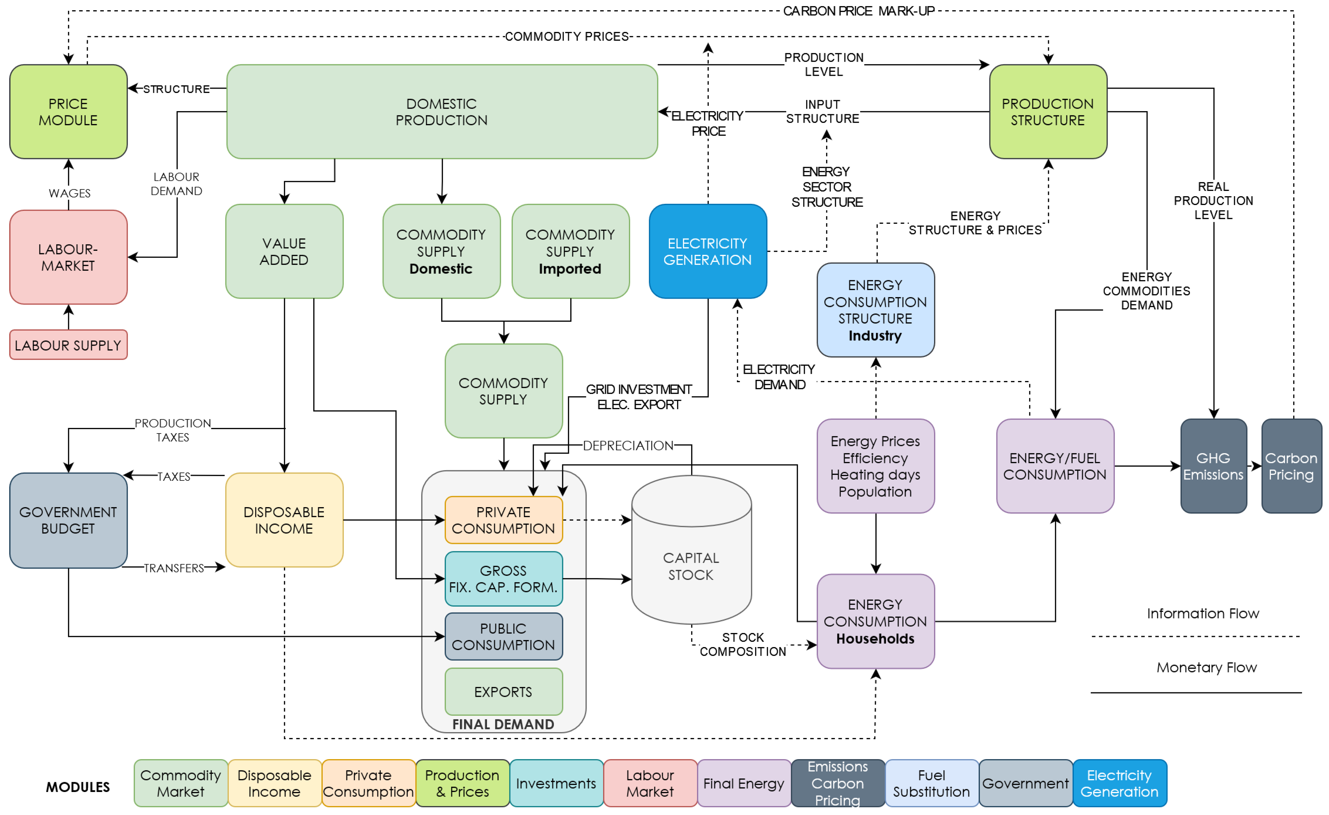
The current model comprises eleven interrelated modules (see Figure 1). The solution process is an iteration over all modules until convergence is achieved. In the following, each module is presented shortly in order to provide an overview of the main features of the model, drivers for the simulations and interactions between different model components. In the description, emphasis is put on the newly developed module “Electricity Generation” (Module 11), for the other modules and data sets used in DYNK a more detailed description can be found in Kirchner et al. [20].

2.1.1. Module 1: Commodity Market

This module represents the Input-Output core of the model. The commodities demanded by public and private consumers, investment and exports are supplied by a set of sectors. The production necessary to satisfy the demand is calculated using a Leontief equation. Thereby it is guaranteed that the demand of commodities equals supply. The results of this module are employment, value added and production value per sector. The data set used are Input-Output-Tables [22] of the Austrian Economy for the year 2017.

2.1.2. Module 2: Disposable Income

Disposable income for private households is derived from value added generated in the sectoral production activities. Pre-defined transfers and unearned income are added, and taxes and social contributions are subtracted using tax rates of the respective year. This yields ’disposable income’ for private households, which is the basis for consumption in the next modules. Data sources are the national Non-Financial-Sector-Accounts [23] of private households for the year 2017.

2.1.3. Module 3: Private Consumption

The consumption decisions of private households (part of final demand) are simulated in this module using several behavioral equations that apply coefficients estimated by time series analysis using Austria-specific data. These equations comprise consumption of energy products (space heating, electricity for appliances and vehicle utilization), durable commodities (housing and vehicles) and a bundle of residual non-durable and non-energy commodities. The commodity composition of this residual bundle is defined by the application of an AIDS (Almost Ideal Demand System). In all equations estimated coefficients and prices define the commodity structure in the respective simulation. The resulting consumption vector is part of final demand and therefore input in Module 1. The applied data comprises a wide range of consumption-related data taken from data bases of EUROSTAT and Statistik Austria (for details see Kirchner et al. [20]).

2.1.4. Module 4: Production and Prices

In this module, a Translog production function specification is applied. The function determines, based on input commodity prices and technology, factor and investment demand as well as output prices. Own- and cross-price elasticities are applied to determine the composition of 5 input-bundles (factors), i.e., Capital (K), Labor (L), Energy (E), Imported commodities (M) and Domestically produced commodities (D), or KLEMD in total. This means that the five factor shares react to relative price constellations whereas the sub-commodity-structure of the factors is constant (Leontief technologies). The principle of the Translog estimations and equations can be found in Sommer and Kratena [8] or in the documentation of FIDELIO2 [24]. The module applies production functions with a Translog specification for each sector. To estimate the coefficients of the Translog equations, system estimations and the Seemingly Unrelated Regression (SUR) estimation method are applied for each specific sector. The coefficients are seen as exogenous in this model. The primary source for the estimations were derived from the WIOD (World Input-Output Database, Release 2013 and 2016) data set that contains World Input Output Tables (WIOT) in current and previous year’s prices, Environmental Accounts (EA), and Socioeconomic Accounts (SEA).

2.1.5. Module 5: Investments

In DYNK, each sector has a specific commodity structure of its investment based on the Input-Output Tables of Statistics Austria. The change in each investment level is linked to the moving average of the economic surplus (factor K) of the sector of the previous 5 years (gross surplus is a part of value added). By this approach, two economic effects are covered. First, the investment needs to satisfy changes in demand (rising production leads to rising value added) and, second, price triggered shifts to the factor capital (and related investments) via the production function (Module 4).

2.1.6. Module 6: Labor Market

The labor market determines the price index for the factor labor, which is one of the five factors in production function (Module 4) and thereby influences the sectoral production prices throughout the economy. The labor market simulates wage negotiations by applying wage curves. These wage curves, in terms of the gross hourly wage rates of the employees, are industry-specific and react to changes in labor productivity and price levels based on econometrically estimated relations. The labor price (index) in the Translog Equations (Module 4) is linked to the developments of these wage rates plus employers’ social security payments.

2.1.7. Module 7: Energy

This module derives the final energy demand of the economy from the economic development. Here the real (i.e., nominal values deflated by the respective gross commodity price) inputs of energy commodities in production and consumption are linked to the physical energy consumption of each sector and households via energy intensity coefficients (Terajoule (TJ) per EUR). The coefficients are deduced from the monetary values in the Input-Output Table and the physical units provided by the Physical Energy Flow Accounts by Statistik Austria [21].

2.1.8. Module 8: Emissions and Carbon Pricing

The energy-related carbon emissions are linked to the energy consumption derived in Module 7 via carbon intensity coefficients, i.e., these emissions are linked to the respective fuel use based on sectoral emissions provided by Statistik Austria [25]. Process emissions that occur due to processes other than combustion are linked to real production values of the respective sectors, again via emission coefficients. An exogenous carbon price is used to infer additional costs for the emissions, i.e., the combustion of fuels or process emissions. The derived costs are used as a mark-up on the commodity taxes system of the Input-Output Tables. Thereby the (gross) prices for specific carbon-containing commodities increase leading to substitution and saving reactions throughout the system. DYNK as a single-region model does not consider the effects of rising carbon prices in other European countries. The reduction in real exports might hence be overestimated as prices in other European countries would rise as well.

2.1.9. Module 9: Fuel Substitution

The sub-structure of commodities of each of the five factors in Module 4 (KLEMD) are constant, i.e., “Leontief technologies”. The sole exception is the factor energy (E), comprising six commodities (CPA05_07 Mining of fossil fuels, CPA16 wood products, CPA19 mineral oil products, CPA35.1 Electricity, CPA35.2 Natural Gas, CPA35.3 District heat). They represent the input of energy in form of coal, oil, gas, electricity, district heat, and renewables in the production process. Five of the six shares of these energy factors are defined by another Translog specification as in Module 4. The share of district heating is unchanged because our Translog specification can only handle 5 factors and the share of district heating in the affected ETS industries is negligible. Hence these factors are also endogenous depending on relative (gross) prices and trends. The main sources for the estimation of the Translog coefficients were EUROSTAT energy balances and WIOD (revision 2016) environmental accounts as well as fossil energy carrier prices from the IEA database. The method here again is a system estimation using the SUR estimation method in order to obtain the parameters of equations of the shares and the unit costs for each specific sector.

2.1.10. Module 10: Government

In module 10, the revenues and expenditures of the regional government are simulated. If expenditures exceed revenues the difference (net lending) is added to the public debt. Only a few elements of revenue and expenditure can be derived from the Supply-Use-Tables structure (taxes in Module 1) and the household’s income composition (taxes in Module 2). Hence, the public household is simulated in a relatively simple fashion. Nevertheless, a mechanism is applied that allows choosing whether public debt is endogenous or exogenous.

2.1.11. Module 11: Electricity Generation

This new module represents the interface to the ATLANTIS model and allows to simulate changes of the annual physical electricity generation (and their costs) in DYNK. A necessity for simulating changes in electricity generation in DYNK was to extract the NACE sector “Electricity generation” from the sector “Electricity, Gas and Heat generation and supply (NACE D35) in all Input-Output Tables of DYNK. This disaggregation has been based on a custom analysis of relevant primary statistics by Statistics Austria. The input structure of the electricity generation sector was then further differentiated into eleven technology-specific cost structures according to the technologies in ATLANTIS plus a residual that represents grid and distribution services. The production value of the eleven technologies is based on the production costs provided by ATLANTIS; their commodity structure is based on the structures of respective electricity generation technologies for Austria in the multi-regional Input-Output Table EXIOBASE (www.exiobase.eu, accessed on 20 February 2023).

The inputs from ATLANTIS are investments in electricity generation technologies, the generation costs of the respective electricity generation mix as well as wholesale price.

The investments in electricity generation technologies are translated into a commodity structure based on literature reviews focusing on the three most relevant technologies for the electricity transition in Austria: wind [26,27,28], hydro [26,29] and PV [26,30,31,32]. The resulting investment vector is then transferred to the electricity sector’s investment in Module 5. The wholesale price of electricity is translated to end-user prices by adding grid costs, fees and taxes. The resulting price determines the output price index of the electricity sector in Module 4. The generation mix defines the commodity input structure of the electricity sector by using weighted input structures for each technology. The weight is determined by the results of ATLANTIS. Furthermore, variations in cost components (costs of operation, fuel, emission permits, labor compensation and depreciation) are considered as well. The adapted input structure is transferred to a change in intermediate inputs of the sector in the Input-Output Tables in Module 1.

2.2. ATLANTIS

In this section, we provide a brief overview of the ATLANTIS model [19] developed at the Institute of Electricity Economics and Energy Innovation (IEE), Graz University of Technology.

ATLANTIS is a techno-economic model of the continental European power system that incorporates both the technical and economic aspects of the power system for long-term scenario simulations. The technical aspects of the model include, inter alia, the continental European electricity system based on 4022 nodes (power stations) with regionalism demand distribution, the transmission grid (including 6864 lines and 1471 transformers), and 79,146 generators (including thermal power plants, renewables, and storage units). The power flow is modeled as direct current (DC) optimal power flow (DC-OPF), which is a good approximation of reality in the transmission grid. Due to the scale of the continental European power system, the temporal framework is based on discretized time duration curves. Since the model is intended for long-term system planning and given the uncertainty of input data over such lengthy time frames, this is reasonable. The economic aspects of the model include, among others, information about electricity companies, fuel prices, and inflation rates to calculate electricity trading between companies, market prices as well as balance sheets and profit and loss accounts for the included companies.

The ATLANTIS model is structured into six different modules, as can be seen on the left side of Figure 2. In the first step, the database and scenarios are implemented. The database includes ATLANTIS-specific information, e.g., the power plants, the transmission network, load profiles, etc. as well as other exogenous parameters that are aligned with the DYNK model such as fuel prices, CO${}_2$ prices, inflation rates, etc.

In the following step, system adequacy is evaluated. This entails assessing whether the winter and summer peak load can be covered with the existing generation capacities given the restrictions of the existing transmission grid (based on a DC-OPF). As a result, a lack of generation and/or transmission capacity is identified.

For this study, each month was divided into two peak and two off-peak periods in order to strike a reasonable balance between accuracy and computational time. ATLANTIS runs two different models per period, where the results of the first model (Zonal Pricing Model) set the initial values for the second one (Redispatch Zonal Pricing Model) for faster model run times. The models are explained in detail in the following sections.

2.2.1. Single Node per Country—Zonal Pricing Model

In the Zonal Pricing (ZP) model, the merit order is calculated per country/zone with the Net Transfer Capacities (NTCs) that cause restrictions in electricity imports and exports between the countries, allowing a coupling between the markets. Within a zone, the cost-optimal dispatch of power plants is calculated by defining a linear optimization problem with the objective of maximising social welfare as defined in Equation (1a). With this, the respective zonal price (market clearing price for each zone) is determined. Trading between ”cheaper“ and "more expensive” zones can thus arise while complying with the commercial restrictions of the NTCs. The ZP-Model provides the zonal price per country/market, the trade flows between the countries/markets as well as the ideal dispatch per power plant (no grid restrictions). The following constraints have to be considered: cleared part of supply has to be smaller than maximum supply in a market (1b); cleared part of demand has to be smaller than maximum demand in a market (1c); limit of trading between two markets based on the defined NTCs (1d); and balance constraint of the markets (1e).

$$\underset{qD,qS}{\max }\left\{\sum _i\left[\sum _n(qD{}_{n,i}·pD{}_{n,i})-\sum _a(qS{}_{a,i}·c{}_{var}S{}_{a,i})\right]\right\}$$

(1a)

subject to:

$$\begin{array}{cc}\begin{array}{cc}\hfill & qS{}_{a,i}\le qS{}_{max{}_{a,i}}\hfill \end{array}\hfill & \hfill \mathrm{(1b)}\\ \begin{array}{cc}\hfill & qD{}_{n,i}\le qD{}_{max{}_{n,i}}\hfill \end{array}\hfill & \hfill \mathrm{(1c)}\\ \begin{array}{cc}\hfill & export{}_{i\to j}-import{}_{i\to j}\le NTC{}_{i\to j}\forall (i,j|i\ne j)\hfill \end{array}\hfill & \hfill \mathrm{(1d)}\\ \begin{array}{cc}\hfill & \sum _{a}qS{}_{a,i}-\sum _{n}qD{}_{n,i}+\sum _{i\ne j}import{}_{i\to j}-\sum _{i\ne j}export{}_{i\to j}=0\forall i\hfill \end{array}\hfill & \hfill \mathrm{(1e)}\end{array}$$

with:

$i,j$	countries, market areas (index)
n	block bid of demand (index)
a	block bid of supply (index)
$q{D}_{n,i}$	cleared part of demand block n in market i [MW]
$q{S}_{a,i}$	cleared part of supply block a in market i [MW]
$p{D}_{n,i}$	demand price [EUR/MWh]
$c_{var}{S}_{a,i}$	marginal costs of supply block a in zone i [EUR/MWh]
$impor{t}_{i\to j}$	import in market i from market j [MW]
$expor{t}_{i\to j}$	export from market i to market j [MW]
$NT{C}_{i\to j}$	net transfer capacity between market i and j [MW]

As this model considers every zone/country as a single node where all the power plants are connected to and all the demand occurs, the dispatch of the power plants does not consider restrictions related to the grid because of congested lines.

2.2.2. Grid Restrictions with DC-OPF—Redispatch Zonal Pricing Model

The Redispatch Zonal Pricing (RDZP) model takes the results of the power plant dispatch from the ZP model as starting values for the solver but incorporates the grid restrictions by implementing a DC-OPF. The DC-OPF is defined as a mixed-integer linear optimization problem with the objective of minimizing overall system costs (2a). The first sum defines the cost of power plant dispatching, the second sum describes the cost of using phase shifting transformers and the third sum defines the penalty costs for cross-market redispatch, that ensures that inner-market redispatch should be used first. (If inner-market redispatch is not enough, the binary variable $H_C^{+}$ switches to 1 to allow cross-market redispatch). Constraint (2b) defines the equilibrium of generation, demand and the power flows to and from a node; (2c) represents the unit commitment (if the power plant is dispatched or not) for thermal power plants; load flow limits of lines are set with (2d) for AC-lines and (2e) for DC-lines; (2f) ensures the power balance between generation demand and export/import per market; (2g) sets the limits for the control angle of phase shifting transformers and (2h) limits the angle of power lines (since the DC load flow is a simplification of the AC load flow, which requires a very small phase angle along a line).

$$\begin{array}{c}\hfill \begin{array}{cc}\hfill \min & \left\{\sum _G{c}_{var,G}·p_G·P_{Base}+\sum _l\left(\alpha ·{\mathsf{\Lambda }}_{l,DC}+\lambda ·{\sigma }_{l,PST}\right)+\sum _C\delta ·H_C^{+}\right\}\hfill \\ \hfill & H_C^{+}\in {\left\{0,1\right\}}_{\mathbb{Z}}\hfill \\ \hfill \end{array}\end{array}$$

(2a)

subject to:

$$\begin{array}{cc}\begin{array}{cc}\hfill & \sum _G{p}_{G,n}-\sum _D{p}_{D,n}=\sum _{m}flo{w}_{n\to m}-\sum _{m}flo{w}_{m\to n}\forall \mathrm{m}\hfill \end{array}\hfill & \hfill \mathrm{(2b)}\\ \begin{array}{cc}\hfill & p_{min,G}\le \beta ·p_G\le p_{max,G}\beta \in {\left\{0,1\right\}}_{\mathbb{Z}}\hfill \end{array}\hfill & \hfill \mathrm{(2c)}\\ \begin{array}{cc}\hfill & -p_{ACmax,l}\le flo{w}_{n\to m}\le p_{ACmax,l}\forall \mathrm{AC}\mathrm{lines}\hfill \end{array}\hfill & \hfill \mathrm{(2d)}\\ \begin{array}{cc}\hfill & -p_{DCmax,l}\le flo{w}_{n\to m}\le p_{DCmax,l}\forall \mathrm{DC}\mathrm{links}\hfill \end{array}\hfill & \hfill \mathrm{(2e)}\\ \begin{array}{cc}\hfill & \sum _G{p}_{G,C}-\sum _D{p}_{D,C}-sald{o}_C^{LF}=0\hfill \end{array}\hfill & \hfill \mathrm{(2f)}\\ \begin{array}{cc}\hfill & -{\sigma }_{max,PST}\le {\sigma }_{l,PST}\le {\sigma }_{max,PST}\forall \mathrm{l}\hfill \end{array}\hfill & \hfill \mathrm{(2g)}\\ \begin{array}{cc}\hfill & -{\mathsf{\Lambda }}_{max,DC}\le {\mathsf{\Lambda }}_{l,DC}\le {\mathsf{\Lambda }}_{max,DC}\forall \mathrm{l}\hfill \end{array}\hfill & \hfill \mathrm{(2h)}\end{array}$$

with:

G	generators (Index)
D	demand (Index)
C	countries, market areas (Index)
$n,m$	nodes (Index)
$c_{var,G}$	marginal costs of generator G [EUR/MWh]
$H_C^{+}$	binary variable to allow cross-border redispatch [−]
$p_{G,n}$	(optimized) feed-in power of generator G at node n [p.u.]
$p_{D,n}$	power demand at node n [p.u.]
$P_{Base}$	power base for per unit calculation [MW]
$\alpha ,\delta ,\lambda$	penalty weights (p.u.)
$\beta$	binary variable for unit commitment [−]
${\sigma }_{l,PST}$	(optimized) angle of phase shifter l, PST [rad]
${\sigma }_{max,PST}$	maximum angle of phase shifter [rad]
$flo{w}_{n\to m}$	active power flow on line l between node n and m [p.u.]
$p_{min,G}$	minimum power of generator G [p.u.]
$p_{max,G}$	maximum power of generator G [p.u.]
$p_{ACmax,l}$	maximum transmission capacity of AC line l [p.u.]
$p_{DCmax,l}$	maximum transmission capacity of DC line l [p.u.]
$sald{o}_C^{LF}$	import/export saldo (result from DC-OPF) [p.u.]
${\mathsf{\Lambda }}_{l,DC}$	(optimized) commitment of DC link l [rad]
${\mathsf{\Lambda }}_{max,DC}$	maximum controlling range of a DC link [rad]

In many countries the heat produced by combined heat and power (CHP) plants is needed in winter months for district heating purposes, making them must-run power plants that have to produce even if they would not be dispatched based on the merit order system. For this model run, power plants with heating output have a must-run flag set in the winter months (November to February) and are therefore forced to produce. According to Austria’s energy balance from Statistics Austria, in 2021 heating demand for district heating was 26 TWh. CHP plants contributed 14.7 TWh, showing the importance of the heat production of CHP plants [33]. Some industrial power plants are also needed throughout the year and, for that reason, have a must-run flag set for the whole year.

In case of line congestions, an intra-zonal redispatch is carried out and, if this is not sufficient, a redispatch across zones is done. In addition to the results of the ZP-Model, the RDZP-Model also provides the line utilization and the “positive” and “negative” redispatch for each power plant.

2.3. Model Linkage

The basis for linking ATLANTIS and DYNK is handling the ATLANTIS model’s output as a disaggregate technological representation of the different electricity sub-sectors. The ATLANTIS solution’s data on electricity generation and distribution of the RDZP model is linked to the corresponding variables in the DYNK model. For example, in ATLANTIS the simulation yields results for fixed (capital) and operational (energy, labor, materials) costs as well as produced electricity per power plant type which is fed into DYNK. The resulting electricity price of the ATLANTIS model is linked to the output price index in DYNK. In the other direction, the resulting electricity demand of DYNK is fed into the ATLANTIS model. This is done until convergence is reached. Due to technical and practical reasons, the data exchanged between ATLANTIS and DYNK comprises full scenario results (up to 2030). Both models were calibrated to the year 2017 and the simulations cover the period from 2017 to 2030.

The different modules of the ATLANTIS model as well as the links between ATLANTIS and DYNK are depicted in Figure 2.

As the models are operated by two different organizations, cloud servers are utilized to exchange the results. An ad hoc data structure based on Excel files was developed for exchanging data between the two models. For this, the data input mechanisms of the two models have been adapted. Likewise, the output of the ATLANTIS model was updated to specifically write the results needed for DYNK (installed capacity, produced electricity, electricity price, and fixed and operational costs, each per power plant type and year) into a single file.

3. Scenario Description

To analyze the effects of the transition to 100% RES-E in Austria (on a national balance), a scenario was developed based on the EAG, explained in more detail in Section 3.1. This Austrian scenario is embedded into a European scenario described in Section 3.2.

3.1. Renewable Expansion Act Scenario

To analyze the effects of the planned generation capacity expansion of the EAG a scenario was developed, where the added capacity is based on the goals and the full load hours (FLH) defined in the EAG. According to the EAG, production from PV should increase by +11 TWh from 2020 to 2030, while production from wind, hydro and biomass should increase by +10 TWh, +5 TWh and +1 TWh, respectively. With the FLH specified in the EAG (PV: 1000 h, wind: 2500 h, hydro <1 MW: 4000 h, hydro >1 MW: 5000 h, biomass: 6850 h) this results in additional capacities of +11000 MW for PV, +4000 MW for wind, +1111 MW of hydro, and +146 MW of biomass that are added linearly from 2020 to 2030. (For hydro power plants, the average FLH of 4500 h was used because it is unknown how many hydro power plants <1 MW and >1 MW will be built in the future. Thus, until the year 2030, 5 TWh is equal to 1111 MW. Additionally, it is assumed that the installed capacity split between run-of-river and (pumped-) hydro storage power plants remains unchanged from 2020 (Run-of-River: 39.6%; (pumped-) hydro storage: 60.4%). Up until 2030, this results in added capacity for run-of-river power plants of +440 MW and +671 MW for (pumped-) hydro storage power plants).

The installed power plant capacities for the scenario can be seen in Figure 3. Between the base year 2017 and 2020, the installed capacities per power plant type are based on E-Control [34]. As the locations of future power plants are not known and not defined in the EAG, but influence the DC-OPF, the following approach has been used: For wind generation, the expansion is based on Gaugl et al. [35], which uses an optimizer to distribute the wind power plants on the basis of the calculated technical expansion potential. PV is distributed according to the population per node with the assumption that rooftop PV systems are preferred to reach the EAG goals. Other power plants are located in already existing locations for that power plant type. This assumption can be made because no new fossil power plants will be added, a large part of the additional run-of-river production will come through revitalization, and existing (pump) storage power plants will be expanded.

With respect to demand-side factors, accelerated electrification and ambitious improvements in energy efficiency are assumed for the household sector. The respective parameters have been determined in a Delphi approach and are based on a comprehensive literature survey (for details see Kettner et al. [36]). It is assumed that the share of heat pumps in total household heating systems increases from 7% in 2017 to 19% in 2030 and that the share of electric cars in total passenger cars rises from 1% to 41% over the same period. Moreover, it is assumed that the specific energy consumption of space heating is reduced from 127 to 86 kWh/m${}^2$, and that fuel consumption of electric cars decreases from 15 to 12 kWh/100 km. For the other areas, past improvements in energy efficiency are extrapolated and changes in the energy mix are the result of changes in the relative prices of the energy sources (see Section 2.1 above).

The assumed fuel prices as well as the prices for CO${}_2$ certificates in the EU Emission Trading System (EU ETS), that covers GHG emissions from energy supply and emission-intensive industry, are referenced in

Table A1. Annual fuel prices used in the simulation.

Year	Crude Oil	Natural Gas	Coal	CO${}_2$
	EUR/MWh	EUR/MWh	EUR/MWh	EUR/t
2017	39	28	14	9
2018	42	32	14	19
2019	46	37	13	29
2020	49	42	12	38
2021	52	43	13	48
2022	56	44	13	58
2023	59	44	14	67
2024	62	45	15	77
2025	66	46	15	87
2026	69	46	16	96
2027	72	47	16	106
2028	76	48	17	116
2029	79	49	17	125
2030	82	50	18	135

. In order to see the effects a higher CO${}_2$ price has on the results of the interlinked model system, sensitivity analyses are performed where the CO${}_2$ price is doubled and tripled from 2021 compared to the CO${}_2$ price in Table A1 (leading to CO${}_2$ prices of 270 EUR/tCO${}_2$ and 405 EUR/tCO${}_2$, respectively, in the year 2030).

3.2. Scenario for the Rest of Continental Europe

As Austria is part of the synchronous grid of Continental Europe it is important to simulate this Austrian scenario in a European context in the ATLANTIS model. For the ATLANTIS model, the information about installed capacity per country per power plant type, demand per country and grid expansion information is necessary. To get an overview of existing scenarios of the European electricity sector, a thorough literature review was done at the beginning of the study. The results can be seen in

Table A2. Overview of the literature review for different European scenarios with remarks about the information needed.

Org.	Publ.	Scenario	Cap./Ctry.	Dem/Ctry.	Grid Exp.	Source
IEA	World Energy Outlook 2020	Stated Policies	No	No	No	[37]
ENTSO-E	TYNDP 2018	Sustainable Transition	Yes	Yes	Yes	[38]
ENTSO-E	TYNDP 2018	Distributed Generation	Yes	Yes	Yes	[38]
ENTSO-E	TYNDP 2018	Global Climate Action	Yes	Yes	Yes	[38]
ENTSO-E	TYNDP 2018	EUCO 2030	Yes	Yes	Yes	[38]
EU	EUCO 2019	EUCO 3232.5	Yes	Yes	No	[39]
WEC	WEC Scenario 2019	Modern Jazz	No	No	No	[40]
WEC	WEC Scenario 2019	Unfinished Symphony	No	No	No	[40]
WEC	WEC Scenario 2019	Hard Rock	No	No	No	[40]
Shell	Shell Scenarios 2018	Sky	No	No	No	[41]
BP	Energy Outlook 2020	Net-Zero	No	No	No	[42]
BP	Energy Outlook 2020	Business-as-Usual	No	No	No	[42]
BP	Energy Outlook 2020	Rapid	No	No	No	[42]
McKinsey	Global Energy Perspective 2019	Reference Case	Yes	Yes	No	[43]
IRENA	Global Renewables Outlook 2020	Planned Energy	No	No	No	[44]
IRENA	Global Renewables Outlook 2020	Transforming Energy	No	No	No	[44]
IRENA	Global Renewables Outlook 2020	Baseline	No	No	No	[44]
Equinor	Energy Perspectives 2020	Reform	No	No	No	[45]
Equinor	Energy Perspectives 2020	Rebalance	No	No	No	[45]
Equinor	Energy Perspectives 2020	Rivalry	No	No	No	[45]

. Since the project began in 2020 newer scenarios published in the meantime could not be considered due to the project timeline. The scenarios that tick off all the boxes needed in the ATLANTIS model are the ones from the Ten Year Network Development Plan (TYNDP) of the European Network of Transmission System Operators for Electricity (ENTSO-E). The Sustainable Transition scenario was chosen for the rest of Continental Europe as it was deemed the most realistic one by the project team as well as by stakeholders and external experts participating in a project workshop on scenario development. It reaches the EU targets through national regulation, emission trading schemes, and subsidies, and therefore maximizes the use of existing infrastructure. Based on this scenario, the corresponding power plant development for each power plant type (considering planned projects), demand trends, and future electricity grid projects were implemented in ATLANTIS.

4. Results and Discussion

This section first describes the iterative process necessary to interlink the two models ATLANTIS and DYNK, and then presents the final results of the interlinked model system for the EAG scenario in Austria as well as the sensitivity analysis examining the effects of a higher CO${}_2$ price.

4.1. Iterative Process

The DYNK and ATLANTIS models are linked as described in Section 2.3 and iteratively solved until convergence, i.e., until the change of electricity demand from the DYNK model does not affect the electricity price in the ATLANTIS model anymore. This process is shown in

Table 1. Results for electricity demand and price for the iterative process.

	Electricity Demand in TWh
Iteration	’17	’18	’19	’20	’21	’22	’23	’24	’25	’26	’27	’28	’29	’30
1	65.8	66.2	66.0	63.6	67.0	68.5	70.4	72.4	74.2	75.6	76.9	77.9	78.8	79.3
2	65.8	66.2	66.0	63.6	67.0	68.4	70.3	72.3	74.0	75.4	76.6	77.6	78.4	78.9
	Electricity Price in EUR/MWh
Iteration	’17	’18	’19	’20	’21	’22	’23	’24	’25	’26	’27	’28	’29	’30
1	27.3	42.6	55.9	67.4	80.3	92.4	99.5	105.3	110.4	116.1	121.9	127.9	133.3	138.3
2	27.3	42.6	55.9	67.4	80.3	92.4	99.5	105.3	110.3	116.1	121.9	127.9	133.3	138.2

for the standard scenario, but the same methodology was used for both scenarios of the CO${}_2$ sensitivity analysis. To start the iterative process, in the first iteration baseline values for the electricity prices are set in the DYNK model starting in 2017 (which was the base year for the simulations). The baseline values already have realistic electricity price assumptions implemented which has the advantage that starting with realistic values reduces the number of iterations until convergence. The resulting electricity demand (Table 1, iteration 1 of electricity demand) is then fed into the ATLANTIS model which results in updated yearly average electricity prices (Table 1, iteration 1 of electricity prices). These new electricity prices are then inserted back into the DYNK model for the second iteration, resulting in a new series of electricity demand (Table 1, iteration 2 of electricity demand). The ATLANTIS model was updated with the new demand and because the resulting electricity prices (Table 1, iteration 2 of electricity prices) are nearly identical to the ones before, the iterative process could be stopped as without a change in electricity prices the outcome of electricity demand in the DYNK model would stay the same (and therefore convergence has been reached). We do not include more iterations in Table 1 as convergence was reached. Depending on how much the results would change between iterations, the iterative process could take longer, but usually, convergence was achieved after two or three iterations.

4.2. EAG Scenario

The models were calibrated for the base year 2017 and the error of the simulated values compared to the real production values from the Austrian Energy Balances [33] is smaller than 6%. This is mostly due to a lower hydro production. As an average hydro year was chosen for the inflows of the hydro power plants, this small error was accepted. For 2017, hydro power plants (sum of run-of-river and hydro (pumped) storage) make up for the biggest part of the electricity production with 35.1 TWh, followed by gas (8.3 TWh) and wind power (7.2 TWh). The development of the electricity production per power plant type for Austria from 2017 to 2030 after achieving convergence of the interlinked model can be seen in Figure 4. Due to the (exogenous) expansion plan defined in the EAG, the basis for this simulation (see Section 3.1), PV and wind power see the largest increase in produced electricity between 2017 and 2030 with gains of +11.7 TWh and +10.6 TWh, respectively. Hydro power still remains the most important source of electricity for Austria accounting for 39.1 TWh. Counter-intuitively, larger RES-E generation also leads to more production from gas-fired power plants, because they have to compensate for the fluctuating generation from renewables. Additionally, with the assumed fuel price developments defined before the energy crisis resulting from the war in Ukraine, gas is cheaper compared to coal. (The project team did address the issue of higher gas prices in a sensitivity analysis which can be found in Kettner et al. [36]). Therefore, Austria is also exporting cheaper electricity from gas-fired power plants (in addition to RES-E) to neighboring countries replacing electricity from coal power plants there.

Currently, Austria’s electricity production is not enough to cover the domestic demand, making it a net importing country, where electricity imports exceed exports over a year. Especially during winter months, when demand is typically higher in Austria and electricity production from run-of-river power plants (Austria’s most important electricity source) is smaller because of lower inflows, Austria has to import electricity from neighboring countries (most importantly Germany). Although electricity demand is assumed to increase to 79.8 TWh in our simulations, Austria is set to become a net-exporting country by 2026. In 2030, Austria is net-exporting 10.7 TWh. Figure 5 shows the monthly electricity production in 2030, showing that the majority of exports occur during the summer months. It can also be seen that run-of-river and PV production are higher in summer, and wind production is higher in winter months. The installed wind capacity is too small to compensate for the decreased run-of-river and PV production in winter and therefore more gas-fired power plants are needed in winter months.

Despite the higher share of renewable electricity, the price for electricity (energy price only; not including taxes or grid tariffs) is still rising to 138 EUR/MWh in 2030 as displayed in Figure 6. With the merit order system in place, where the last power plant needed to cover the demand is setting the wholesale market price, gas-fired power plants are the price-setting technology in most of the simulated periods, though a small flattening of the electricity price curve can be seen in Figure 6 with a rising share of renewables.

4.3. CO${}_2$ Sensitivity Analysis

In the sensitivity analysis of the CO₂ price, we double and triple the CO₂ price starting from 2021. The results shown in this chapter are the final results after the linked model system has reached convergence. With higher CO${}_2$ prices reaching 270 EUR/tCO${}_2$ and 405 EUR/tCO${}_2$ in 2030, the electricity price increases to 197 EUR/MWh and 249 EUR/MWh, respectively, as shown in Figure 6. The electricity prices in 2030 for the CO₂ 270 scenario are 42% higher compared to the standard EAG scenario and for the CO₂ 405 scenario this means a 79% increase.

The higher electricity prices lead to a reduction of electricity demand (mainly due to a decrease in production activities) as can be seen in Figure 7. This decrease is much smaller (−2% for the 270 EUR/tCO${}_2$ scenario and −3% for the 405 EUR/tCO${}_2$ scenario) than the increase in the wholesale electricity price. This reflects on the one hand that the increase in consumer prices is lower than the increase in wholesale prices as these account only for one part of the prices paid by households and companies, and other price components such as grid charges are assumed to remain unchanged. On the other hand, for the household sector electrification follows a predefined pathway (see Section 4.2) and for the industry sector a rising carbon price in the EU ETS does not only increase electricity prices but also—and even more pronouncedly—the costs of using gas, oil or coal, so that firms have no incentives to switch to these fuels. Finally, electricity demand is quite inelastic and so even big changes in electricity prices have only a small impact on the electricity demand when capital stocks are fixed. In the long run, the price elasticity of electricity demand can be assumed to be higher than the short run. This has the potential to further reduce electricity demand.

Higher CO${}_2$ prices lead to lower demand, but also to (a little) higher production from gas-fired power plants in Austria and higher net exports (Figure 8). This is due to the fact, that in the European scenario, other countries still have operating coal-fired power plants. As these are much more affected by the higher CO${}_2$ prices (because they emit much more CO${}_2$ per produced MWh), coal generation is largely being replaced by gas generation. Furthermore, as demand is decreasing in Austria with higher CO${}_2$ prices, the amount of electricity not used in Austria is also exported and replaces more expensive electricity in other countries.

5. Conclusions

By using the novel approach of interlinking the technical model of the Continental European electricity system ATLANTIS with the macroeconomic model DYNK we are able to assess the socio-economic impact of changes in the electricity price. The results show that gas-fired power plants are becoming even more important with higher shares of RES-E, as the fluctuating output of renewables requires controllable power plants. Therefore, gas-fired power plants will still set the market price for electricity in the merit order, leading to higher electricity prices in the future. Other solutions, like demand side management, could help accommodate variable RES-E generation but have not been included in this study. In the EAG scenario, GDP increases by 18% in 2030 compared to 2017, mainly due to increases in population, exports and total factor productivity, and final electricity demand increases by 20%. The sensitivity analyses with higher CO${}_2$ prices result in even higher electricity prices and decreasing GDP growth rates, which leads to a small decline in electricity demand compared to the EAG scenario. In order to completely decarbonize the Austrian electricity system even more renewables and more storage would be needed than stated in the EAG so that surplus electricity could be stored for times of low RES-E production.

References

1. European Commission. The European Green Deal; COM(2019)640; European Commission: Brussels, Belgium, 2019. [Google Scholar]
2. United Nations. Paris Agreement to the United Nations Framework Convention on Climate Change; T.I.A.S. No. 16-1104; United Nations: New York, NY, USA, 2015. [Google Scholar]
3. European Commission. ‘Fit for 55’: Delivering the EU’s 2030 Climate Target on the Way to Climate Neutrality; COM(2021) 550; European Commission: Brussels, Belgium, 2021. [Google Scholar]
4. European Commission. REPowerEU Plan; COM(2022) 230; European Commission: Brussels, Belgium, 2022. [Google Scholar]
5. Oesterreichischer Nationalrat. Erneuerbaren-Ausbau-Gesetzespaket—EAG-Paket; BGBl. I Nr. 150/2021; Oesterreichischer Nationalrat: Vienna, Austria, 2021. [Google Scholar]
6. UBA (Environment Agency Austria). Energiewirtschaftliche Szenarien im Hinblick auf Klimaziele 2030 und 2050; UBA (Environment Agency Austria): Vienna, Austria, 2017; ISBN 978-3-99004-445-2. [Google Scholar]
7. Kratena, K.; Meyer, I.; Sommer, M. Alternative Szenarien zur Entwicklung des Energieverbrauchs in Österreich. Der Einfluss der CO2- und Energiepreise bis 2030. WIFO-Monatsberichte 2014, 87, 427–441. [Google Scholar]
8. Sommer, M.; Kratena, K. The Carbon Footprint of European Households and Income Distribution. Ecol. Econ. 2017, 136, 62–72. [Google Scholar] [CrossRef] [Green Version]
9. UBA (Environment Agency Austria). GHG Projections and Assessment of Policies and Measures in Austria; UBA (Environment Agency Austria): Vienna, Austria, 2019; ISBN 978-3-99004-506-0. [Google Scholar]
10. Bachner, G.; Bednar-Friedl, B.; Feichtinger, F.; Gobiet, A.; Gutschi, C.; Heinrich, G.; Kulmer, V.; Leuprecht, A.; Prettenthaler, F.; Rogler, N.; et al. ElAdapt—Impacts of Climate Change and Adaptation in the Electricity Sector; Wegener Center Verlag: Graz, Austria, 2019; ISBN 978-3-9503112-8-0. [Google Scholar]
11. Bussar, C.; Stöcker, P.; Cai, Z.; Moraes, L., Jr.; Magnor, D.; Wiernes, P.; van Bracht, N.; Moser, A.; Sauer, D.U. Large-scale integration of renewable energies and impact on storage demand in a European renewable power system of 2050—Sensitivity study. J. Energy Storage 2016, 6, 1–10. [Google Scholar] [CrossRef] [Green Version]
12. Zappa, W.; Junginger, M.; van den Broek, M. Is a 100% renewable European power system feasible by 2050? Appl. Energy 2019, 233–234, 1027–1050. [Google Scholar] [CrossRef]
13. Child, M.; Kemfert, C.; Bogdanov, D. Flexible electricity generation, grid exchange and storage for the transition to a 100% renewable energy system in Europe. Renew. Energy 2019, 139, 80–101. [Google Scholar] [CrossRef]
14. Zhong, J.; Bollen, M.; Rönnberg, S. Towards a 100% renewable energy electricity generation system in Sweden. Renew. Energy 2021, 171, 812–824. [Google Scholar] [CrossRef]
15. Krajačić, G.; Duić, N.; da Graça Carvalho, M. How to achieve a 100% RES electricity supply for Portugal? Appl. Energy 2011, 88, 508–517. [Google Scholar] [CrossRef]
16. Fernandes, L.; Ferreira, P. Renewable energy scenarios in the Portuguese electricity system. Energy 2014, 69, 51–57. [Google Scholar] [CrossRef] [Green Version]
17. Krakowski, V.; Assoumou, E.; Mazauric, V.; Maïzi, N. Feasible path toward 40–100% renewable energy shares for power supply in France by 2050: A prospective analysis. Appl. Energy 2016, 171, 501–522. [Google Scholar] [CrossRef]
18. Child, M.; Bogdanov, D.; Breyer, C. The Baltic Sea Region: Storage, grid exchange and flexible electricity generation for the transition to a 100% renewable energy system. Energy Procedia 2018, 155, 390–402. [Google Scholar] [CrossRef]
19. Stigler, H.; Bachhiesl, U.; Nischler, G.; Feichtinger, G. ATLANTIS: Techno-economic model of the European electricity sector. Cent. Eur. J. Oper. Res. 2015, 24, 965–988. [Google Scholar] [CrossRef] [Green Version]
20. Kirchner, M.; Sommer, M.; Kratena, K.; Kletzan-Slamanig, D.; Kettner-Marx, C. CO2 taxes, equity and the double dividend—Macroeconomic model simulations for Austria. Energy Policy 2019, 126, 295–314. [Google Scholar] [CrossRef]
21. Statistik Austria. Physische Energieflussrechnung 2017 Österreich; Statistik Austria: Vienna, Austria, 2021. [Google Scholar]
22. Statistik Austria. Input-Output-Tabellen 2017 Österreich; Statistik Austria: Vienna, Austria, 2021; ISBN 978-3-9503112-8-0. [Google Scholar]
23. Statistik Austria. Nichtfinanzielle Sektorkonten, Sektor Private Haushalte 2017 Österreich; Statistik Austria: Vienna, Austria, 2021. [Google Scholar]
24. Streicher, G.; Salotti, S.; Valderas, J.; Sommer, M.; Kratena, K. FIDELIO 2—Overview and Theoretical Foundations of the Second Version of the Fully Interregional Dynamic Econometric Long-Term Input-Output Model for the EU-27; Publications Office of the EU: Luxembourg, 2017. [Google Scholar] [CrossRef]
25. Statistik Austria. Luftemissionsrechnung 2017 Österreich; Statistik Austria: Vienna, Austria, 2021. [Google Scholar]
26. Resch, G.; Burgholzer, B.; Totschnig, G.; Lettner, G.; Auer, J.; Geipel, J.; Haas, R. Stromzukunft Österreich 2030—Analyse der Erfordernisse und Konsequenzen eines Ambitionierten Ausbaus Erneuerbarer Energien. Endbericht; Technical Report; TU Wien: Vienna, Austria, 2017. [Google Scholar]
27. Kaltschmitt, M.; Özdirik, B.; Reimers, B.; Schlüter, M.; Schulz, D.; Sens, L. Stromerzeugung aus Windenergie. In Erneuerbare Energien: Systemtechnik · Wirtschaftlichkeit · Umweltaspekte; Kaltschmitt, M., Streicher, W., Wiese, A., Eds.; Springer: Berlin/Heidelberg, Germany, 2020; pp. 461–582. [Google Scholar] [CrossRef]
28. Wallasch, A.K.; Lüers, S.; Heyken, M.; Rehfeld, K. Vorbereitung und Begleitung bei der Erstellung eines Erfahrungsberichts gemäß § 97 Erneuerbare-Energien-Gesetz. Teilvorhaben II e): Wind an Land; Technical Report; Deutsche WindGuard GmbH: Varel, Germany, 2019. [Google Scholar]
29. Aufleger, M.; Joos, F.; Jorde, K.; Kaltschmitt, M.; Rödl, A.; Schlüter, M.; Sens, L. Stromerzeugung aus Wasserkraft. In Erneuerbare Energien: Systemtechnik · Wirtschaftlichkeit · Umweltaspekte; Kaltschmitt, M., Streicher, W., Wiese, A., Eds.; Springer: Berlin/Heidelberg, Germany, 2020; pp. 583–683. [Google Scholar] [CrossRef]
30. Biermayr, P.; Dißauer, C.; Eberl, M.; Enigl, M.; Fechner, H.; Fürnsinn, B.; Jaksch-Fliegenschnee, M.; Leonhartsberger, K.; Moidl, S.; Prem, E.; et al. Innovative Energietechnologien in Österreich Marktentwicklung 2020; Technical Report; Federal Ministry for Climate Action, Environment, Energy, Mobility, Innovation and Technology (BMK): Vienna, Austria, 2021. [Google Scholar]
31. Bründlinger, R.; Christ, D.; Fechner, H.; Kaltschmitt, M.; Müller, J.; Peharz, G.; Schulz, D.; Sens, L. Photovoltaische Stromerzeugung. In Erneuerbare Energien: Systemtechnik · Wirtschaftlichkeit · Umweltaspekte; Kaltschmitt, M., Streicher, W., Wiese, A., Eds.; Springer: Berlin/Heidelberg, Germany, 2017; pp. 339–460. [Google Scholar] [CrossRef]
32. Fechner, H. National Survey Report of PV Power Applications in Austria 2020; Technical Report; IEA: Paris, France, 2021. [Google Scholar]
33. Statistik Austria. Gesamtenergiebilanz Österreich; Statistik Austria: Vienna, Austria, 2021. [Google Scholar]
34. E-Control. Bestandsstatistik Kraftwerkspark Jahresreihen; E-Control: Vienna, Austria, 2021. [Google Scholar]
35. Gaugl, R.; Klatzer, T.; Bachhiesl, U.; Wogrin, S.; Jodl, S. GIS-based optimization—Achieving Austria’s 2030 wind energy target. Elektrotech. Inftech. 2021, 138, 590–596. [Google Scholar] [CrossRef]
36. Kettner, C.; Böheim, M.; Sommer, M.; Gaugl, R.; Bachhiesl, U.; Gruber, L.; Klatzer, T.F.; Wogrin, S.; Kratena, K. Transformation to a Renewable Electricity System in Austria: Insights from an Integrated Model Analysis; START2030 Working Paper #2; WIFO: Vienna, Austria, 2023. [Google Scholar]
37. IEA. World Energy Outlook 2020; IEA: Paris, France, 2020. [Google Scholar]
38. ENTSO-E. TYNDP2018—Scenario Report; ENTSO-E: Brussels, Belgium, 2018. [Google Scholar]
39. European Commission. Results of the EUCO3232.5 Scenario on Member States; Technical Note; European Commission: Brussels, Belgium, 2019. [Google Scholar]
40. World Energy Council. World Energy Scenarios 2019: Exploring Innovation Pathways to 2040; World Energy Council: London, UK, 2019. [Google Scholar]
41. Shell International B.V. Shell Scenarios Sky—Meeting the of the Paris Agreement; Shell International BV: The Hague, The Netherlands, 2018. [Google Scholar]
42. BP. Energy Outlook 2020 Edition; BP: London, UK, 2020. [Google Scholar]
43. McKinsey Solutions SPRL. Global Energy Perspective 2019: Reference Case; McKinsey Solutions SPRL: Bruxelles, Belgium, 2019. [Google Scholar]
44. IRENA. Global Renewables Outlook: Energy Transformation 2050 (Edition: 2020); International Renewable Energy Agency: Abu Dhabi, United Arab Emirates, 2020; ISBN 978-92-9260-238-3. [Google Scholar]
45. Equinor. Energy Perspectives; Equinor: Stavanger, Norway, 2020. [Google Scholar]
Figure 1. Structure of the DYNK model.
Energies 16 02229 g001
Figure 2. Flow chart of the model system showing the structure of the ATLANTIS model on the left side, the DYNK model on the right side and the interlinks between the models.
Energies 16 02229 g002
Figure 3. Development of the installed capacities per power plant type for Austria from 2017 to 2030.
Energies 16 02229 g003
Figure 4. Development of the produced electricity per power plant type, net import/export and demand for Austria from 2017 to 2030.
Energies 16 02229 g004
Figure 5. Monthly produced electricity per power plant type in Austria for 2030.
Energies 16 02229 g005
Figure 6. Annual average electricity prices in the EAG scenario and in the CO 2 price sensitivity analysis.
Energies 16 02229 g006
Figure 7. Demand in the EAG scenario and in the CO 2 price sensitivity analysis.
Energies 16 02229 g007
Figure 8. Produced electricity per power plant type in 2030 for the three different scenarios.
Energies 16 02229 g008