Will NILM Technology Replace Multi-Meter Telemetry Systems for Monitoring Electricity Consumption?

Abstract

The estimation of electric power utilization, its baseload, and its heating, light, ventilation, and air-conditioning (HVAC) power component, which represents a very large portion of electricity usage in commercial facilities, are important for energy consumption controls and planning. Non-intrusive load monitoring (NILM) is the analytical method used to monitor the energy and disaggregate total electrical usage into appliance-related signals as an alternative to installing multiple electricity meters in the building. However, despite considerable progress, there are a limited number of tools dedicated to the problem of reliable and complete energy disaggregation. This paper presents an experiment consisting in designing an electrical system with electrical energy receivers, and then starting NILM disaggregation using machine learning algorithms (MLA). The quality of this disaggregation was assessed using dedicated indicators. Subsequently, the quality of these MLA was also verified using the available BLUED data source. The results show that the proposed method guarantees non-intrusive load disaggregation but still requires further research and testing. Measurement data have been published as open research data and listed in the literature section repository.

1. Introduction

With the growing demand for electricity and the growing awareness of society about the effects of unsustainable development, there is a need for an in-depth analysis of electricity consumption by both individual and business consumers [1]. The purpose of such an analysis is to indicate the possibilities of reducing the volume and costs of energy consumption by observing consumption, analyzing information and data, drawing conclusions, implementing real optimization activities and consumption forecasting [2]. A typical analysis of electricity consumption for the entire building, which is based on monthly readings of consumption values on the main line supplying the facility (main power input; MPI) is not an appropriate approach in this case, because it does not provide satisfactory information about energy consumption from both the main line and through individual sub-circuits [3,4], e.g., lighting, ventilation, air conditioning, heating, etc. Even when MPI measurements are concentrated to more frequent readings, e.g., every 15 min, only a detailed insight into energy consumption in specific sub-circuits opens wide opportunities to verify the current state and take optimization actions [5,6]. The risk is that with more meters, their potential failures may result in incorrect data [7].

In practical implementations of telemetry systems for measuring electricity consumption (appliance load monitoring; ALM), several solutions can be found, which are divided into intrusive (intrusive load monitoring; ILM) and non-intrusive (non-intrusive load monitoring; NILM) methods. In the first method, measurement systems with one measurement point at the MPI supply line (single-meter measurement systems) are used, sometimes with additional meters at terminals of each device or at a separated sub-circuit (multi-meter measurement systems) [8]. This means that single-meter systems are in some cases extended by further measurement points as physical electricity meters installed on isolated sub-circuits. In such configurations, data are read locally and then aggregated data are transmitted to IT application/database. The other intrusive category consists of advanced metering infrastructure (AMI) analyzers, enabling remote readings of electricity consumption from one or many meters (energy consumption reading) and monitoring of network quality parameters.

The use of many meters for monitoring electricity consumption introduces numerous limitations. In the case of local readings, it is necessary to be physically present at the meters and note the electricity consumption values. Remote measurements are a significant facilitation, but require collecting data locally, processing and sending them to the analytical server using available transmission technologies. The economic aspect is an important limitation as increasing the measurement points requires the installation of more electricity meters and the necessary peripheral devices (more current transformers and cabling), which increases the cost of metering the entire system. In addition, all data must be collected in a local central unit and sent to analytical servers, which generates the need to provide wired or wireless data transmission. It should also be noted that the expansion of the measuring system causes an increase in electricity consumption for powering the measuring system itself. Multi-counter ILM systems enable monitoring energy consumption in individual sub-circuits, which facilitates taking optimization measures in these sections.

In recent years, attempts have been made to replace multi-counter measurement systems with non-intrusive technologies, in which the physical separation of sub-circuits or devices has been replaced with algorithms for data analysis obtained because of high-frequency sampling of the MPI signal. Among the available technologies, NILM (also known as NIALM; non-intrusive appliance load monitoring) should be distinguished, first proposed by Hart et al. [9]. NILM is a technology for separating a household’s aggregate electricity consumption information. Although this technology was developed in 1992, its practical usage and mass deployment since then have been rather limited, possibly because the commonly used datasets are not adequate for NILM research [5]. This method requires the installation of only one electricity meter located on the main supply line (Figure 1). The monitored signal is sampled, and analytical algorithms are designed to separate the signals of devices operating within the collective signal. If a new device is connected to the network, there is no need to install additional physical meters (as is the case in ALM systems), because well trained analytical algorithms can indicate subsequent devices as part of the collective MPI signal.

Previous studies have shown that the practical application of NILM technology has some disadvantages, as the detection of electrical devices in collective signals is still limited and imperfect [8,10,11,12]. The subject of this research is the experimental verification of whether and to what extent NILM can replace multimeter measurement systems. Taking up the topic is justified due to the above-mentioned limitations of intrusive methods. The following research questions were formulated:

• How can we identify and separate the measurement components of individual devices included in the collective signal?
• Why has NILM technology not replaced multi-meter metering systems so far?

The inspiration for the research was to check the effectiveness of artificial intelligence algorithms enabling NILM decomposition at a high level of device identification. The selected experimental research method is used in the study of phenomena that should be traced as occurring on the time axis and the researcher has control over the experiment and can directly, precisely, and systematically manage its course. The presented method, in particular the measurement system, used algorithms, and created dataset, represents a comprehensive approach to NILM. The novelty is the method of conducting the experiment and the results obtained: the NILM measurement system was designed, and then artificial intelligence algorithms were used to disaggregate the signal, the selection of which was adjusted to the characteristics of the collected data. The algorithms were compared using characteristic measures (precision, recall, F-measure) and the collected measurement data were made publicly available under the name SESNED. Then, the effectiveness of the algorithms was re-verified on the available, public BLUED dataset.

The structure of this paper is as follows: After the introduction, the theoretical foundations of NILM are presented. The next section contains a description of the research methodology, and the following section describes the method of conducting the experiment. In Section 6, the algorithms used for the analysis of experimental data are validated by an analysis of data from the NILM open data source BLUED. The last part of this paper contains conclusions, implications, limitations, and future work. The results presented in this publication are a part of the research project “SESCOM’s Business Intelligence Platform for energy saving and smart facility management”.

2. State of the Art Analysis

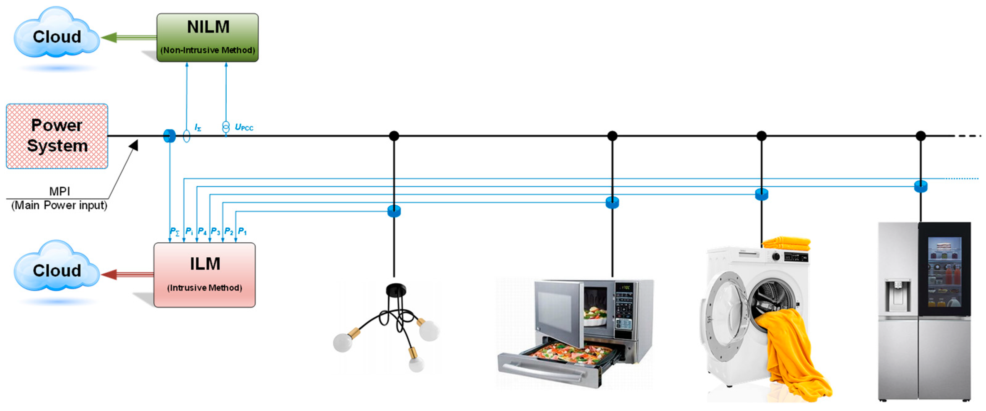
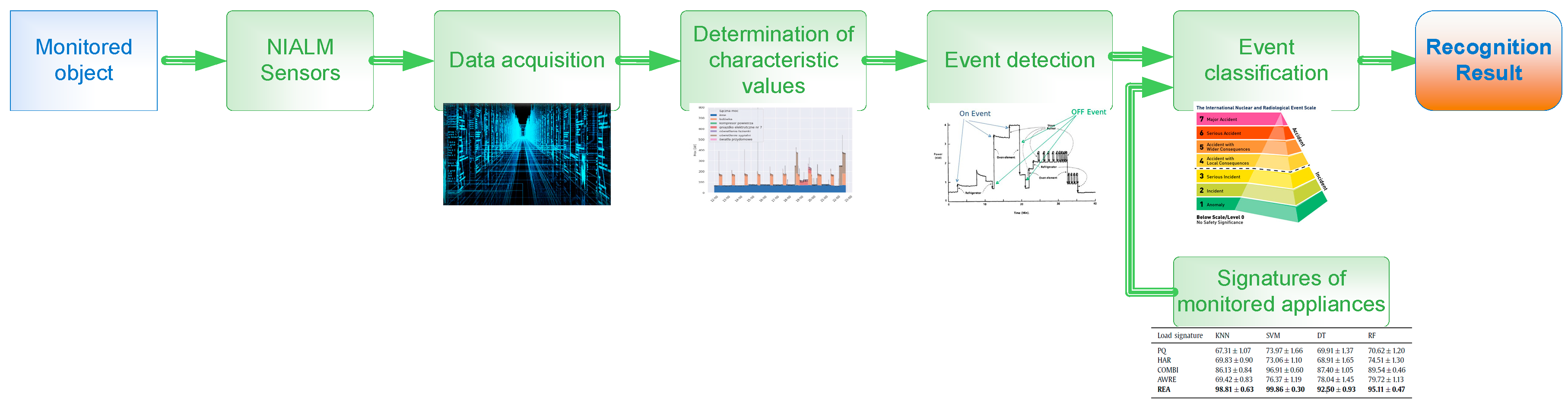
2.1. NILM System Structure

Nowadays, information on the current level of electricity consumption is obtained from electricity meters using digital signal processing methods. One of the key challenges for NILM systems is to select the appropriate current and voltage measurement parameters for further processing. On the one hand, the higher sampling frequency of measurements allows for the identification of a larger spectrum of characteristic indicators describing energy consumption. On the other hand, higher costs are associated with data processing, transmission, and storage. The components of a typical NILM system are shown in Figure 2.

The first stage of the NILM system is the meter (Figure 2), whose main task is to measure a given electrical quantity (voltage, current). Then, during sampling and data acquisition, the measured values are saved in the computer memory and then in the cloud. The next step is to determine the characteristic values (the so-called signatures) that allow the identification of devices and the estimation of their status. The ability to select characteristic values is determined mainly by the sampling frequency of the measurement system. Usually, the following division is adopted:

• low frequency measurements (0–60 Hz),
• medium frequencies measurements (1–50 kHz),
• high frequency measurements (0.5–50 MHz).

Before starting the NILM system, it is necessary to identify the characteristic behaviors for each of the devices. In NILM systems, devices can be classified by their mode of operation:

• Two-state devices: devices whose operating status can be one of two values (on/off) with one time-independent operating parameter (usually it is power).
• Discrete devices which operating status can be inactive or active in one of countable values of time independent parameter (n − 1 value of power).
• Devices with an infinite number of states: Devices whose power consumption changes smoothly and can be different between their subsequent activations. This is the class of devices that is most difficult to identify due to their variable nature. Determining a profile that would allow to develop a signature that is constant during the use of such a device is very demanding [13].
• Constant energy consumers: devices that have only one permanent mode of operation.

The next step is to detect the event, e.g., based on changes in characteristic values in subsequent data frames. Since many devices can operate at the same time, most NILM methods recognize only the last device that changed its status, and then, looking at the power drawn from the network and the status of other devices, determine the power consumed by the device that triggered the new event.

2.2. Signatures and Characteristic Values

Each of the electrical devices is characterized by a profile called a signature. In the early 1990s [9], a method was developed to recognize switched-on devices using active and reactive power as signatures. In later years, it was proposed to use other characteristic values, such as transient waves [14], harmonics spectrum [15], current and voltage [16], electromagnetic interference spectrum, power-on interference spectrum [17], and the starting current [18]. Many of the NILM methods, in addition to examining the signatures for single devices [19], also examine the values characteristic for all possible combinations of devices in order to facilitate the identification of groups of devices. It should also be mentioned that, in addition to methods that use steady states of the system, there are also those that use transient states [14,16,20].

2.3. Macroscopic Signatures

Signatures obtained from low-frequency measurements (below fn—rated frequency of power supply) give the opportunity to know macroscopic features, such as active and reactive power. Research conducted at EPRI (Electric Power Research Institute) and MIT (Massachusetts Institute of Technology) [8,15,21] found that signatures based on active and reactive power can be used to identify and disaggregate signals of electrical devices, including device transients during startup. In publications [22,23], it was proposed to add values based on the slopes and edges of the current intensity signals to the signature, which would help solve the problem of identifying transients in the case of devices that have a long start-up time, e.g., electric motors.

2.4. Microscopis Signatures

Signals and features obtained during measurements with a higher frequency (>fn) are called signatures at the micro level and allow to know the so-called microscopic features [24]. Microscopic signatures are harmonic values and include the Fourier transform of the signal, Fourier transform of the noise signal, signals in the time domain, etc. The use of these signatures requires the use of high-end sensors and expensive equipment for collecting data at high frequency. The authors in [15] proposed adding higher harmonics as the third dimension of the ΔP-ΔQ plane, which shows the dependence of active power changes as a function of reactive power changes. This provides additional characteristic values, which allow to distinguish two devices having identical signatures on the ΔP-ΔQ plane. Most often, the use of higher harmonics is limited to the 11th harmonic level. The information that harmonics provide is most helpful in identifying non-linear devices with non-sinusoidal current flow. To improve the recognition of devices with variable load, in the study [25] the authors used the first few STFT (short-time Fourier transform) factors as an extension of harmonic information. In turn, in [20], the noise spectrum of the measured voltage signal was used to detect sudden changes in the signal that occur when new devices are connected to the grid and switched on. This approach allows devices to be identified in the frequency domain when their transient features occur simultaneously in the time domain. However, this solution requires a transient noise analysis, which is computationally very expensive. It is necessary to train the NILM system for each device in all possible combinations of operating devices, which is time consuming to both measure and calculate. In addition to harmonics and the Fourier transform, other signatures are also used in disaggregation, e.g., the wavelet transform, the geometric shape of the current-voltage curve [26,27], and the transient energy [28]. The wavelet transform represents the physical behavior of the load in the transient state and provides information about simultaneous location versus time and frequency, which cannot be provided by the Fourier transform [8]. It is worth mentioning that to improve the results of identification and disaggregation, it is advisable to use many different signatures, as indicated by the authors in [24].

2.5. Unconventional Signatures

Less conventional signatures are used in new research into NILM systems. These signatures are used to provide the NILM system with additional information about the operation of the device that is not contained in the previously mentioned signatures. An example of such signatures is time, time of day, temperature, and light intensity [29,30].

2.6. Disaggregation Algorithms

The purpose of the disaggregation algorithms is to recognize devices that are included in the aggregated total load signal. The literature indicates many different disaggregation algorithms based on machine learning, which can be broadly divided into two groups: supervised learning and unsupervised learning. The supervised learning approach requires that the classifier be trained using data with information about all active devices. This analytical approach makes it difficult to detect new devices in the system. Therefore, each extension requires re-training the algorithm and teaching to identify and distinguish/isolate operating load components. In recent years, there has been an increase in the popularity of methods that use unsupervised learning techniques [8]. These methods do not require the use of descriptive data. In this class of algorithms, probabilistic models, such as the factorial hidden Markov model (FHMM), can be used to simulate device behavior. Other methods also deploy machine learning techniques, such as sparse coding [31]. The disadvantage of solutions using unsupervised learning methods is that they provide less information, while their great advantage is the ease of implementation [32].

2.7. Supervised Learning Algorithms

Supervised learning methods require the preparation of a labeled dataset. Supervised systems can be trained both online and offline [8]. In the case of online learning, data are tagged in real time and used for learning at the same time. In the case of offline learning, devices are monitored in a special environment according to a previously developed scenario.

Assembling a measurement unit for each device to obtain data is usually a costly and time-consuming endeavor. In an alternative approach, presented in [33], devices are turned on sequentially to study their effect on the aggregate load. Currently, there are several datasets available on the Internet that have tagged data for many household appliances (see Section 2.12), allowing researchers to train machine learning models without going through a tedious data collection procedure. In addition, using the same data allows to compare the effectiveness of different methods and algorithms.

Supervised learning algorithms can be divided into two groups: pattern recognition algorithms and optimization methods. The former are based on identifying devices when a new device is detected, while the latter do not require the occurrence of events as they carry out identification of the network status in a continuous mode.

Deep neural networks (DNNs) have been successfully applied to energy disaggregation in a supervised way. DNNs can inherently learn the discriminative signatures of the different appliances [34]. These methods try to automatically reveal the temporal structure embedded in the observation data [35]. Zhang at al. investigated several DNNs, such as autoencoders and seq2seq learning [36], and further proposed a sequence-to-point (seq2point) network to handle the energy disaggregation problem. Pan et al. [37] proposed a sequence-to-subsequence (seq2subseq) learning in NILM, which makes a trade-off between seq2seq and seq2point learning.

2.8. Event-Based Algorithms

The original NILM algorithm proposed in [33] was based on pattern recognition. Methods that work this way are usually based on the following three steps: event detection, feature extraction, and pattern matching. The detection of the event consisted in identifying one of the available variations by the edge detector.

In subsequent, more developed methods, it was proposed to use other event detection criteria: detection of sudden jumps, ramps, small oscillations [23], large oscillations [38] and power fluctuations [39]. After detecting an event (turning on a newly connected device in the network), the required features are extracted, and then the inferred features are matched to a pattern consistent with the signature database. To match the new feature vector to the cluster consistent with the feature vector of a given device, the authors in [33] used the maximum likelihood estimator (MLE). In studies [24,40], the use of the Bayesian approach was proposed. It consists in the fact that based on changes in the power level and characteristics corresponding to a given change in the state of the entire system, the so-called naive Bayes classifier. A set of trained binary classifiers should identify all devices. The authors in [8] noted, however, that this method works properly only when it can be ensured that the state of all devices in the system is not correlated, which is not always a realistic assumption.

In the study [8], an example of identifying switched-on devices based on information about the course of active and reactive power can be found. Clustering was used as a HTA (histogram thinning approach) method. Compared to Bayesian methods, Bayesian classifiers perform better in the case of consumers characterized by historical electricity consumption.

When it is required to recognize many devices, it is recommended to use machine learning with supervised learning. These methods allow to build any vector of features containing both time information and transitions between states [41]. One of the most popular methods in this category are artificial neural networks (ANN) [42] and hidden Markov models (HMM) [43]. The effectiveness of methods using machine learning strongly depends on the choice of features that are to be included in the signature. Learning NILM systems based on machine learning requires large computational resources which grow with the growth of the feature vector and the number of devices to study. It typically requires much more tagged data than other methods and adding a new device requires retraining the entire system.

K-nearest neighbors (k-NN) algorithms are used in situations, where there are many unlabeled devices [44]. Another popular solution is the use of support vector machines (SVM) [44,45,46]. In the study [46], the authors propose the use of SVM classifiers together with GMM (Gaussian mixture model) classifiers to create hybrid classifiers. In the SVM/GMM classifier, the GMM demonstrates how the current waveforms are distributed, and the SVM classifies the calculated power characteristics [8]. To improve the operation of classifiers, various algorithms can be combined to create hybrid models, which were presented by [24].

Random forest [47] is an estimator that produces a series of decision trees for multiple subsamples of the training set. By averaging multiple values from multiple decision trees, prediction is improved and the overfitting to the training set that occurs when using single random trees for classification is reduced. The main metaparameter of this algorithm is the number of binary trees used. When learning random forest parameters, two metrics are most used: the Gini index or entropy [48].

2.9. Optimization Methods

Another category of supervised learning algorithms are optimization algorithms, also called eventless algorithms. An example of such an algorithm is the method proposed in [49]. This method tries to find the best match between the unknown measured aggregate load and the known load in the database. Matching uses features extracted from loads coming from one or more devices. Several other methods, including integer programming and genetic algorithms, can be found in the literature [49,50,51]. The main challenges in implementing optimization methods are the simultaneous disaggregation of combinations of many devices and failure to correctly recognize the device due to the similarity to more than one load pattern in the reference database. The problem of complexity increases to a critical level when unknown loads appear in the aggregated signal, because in this case it is not possible to identify any of the devices.

2.10. Unsupervised Learning Algorithms

Unsupervised learning algorithms in the context of NILM have been used relatively recently, hence the amount of literature on the subject is not as extensive as in the case of supervised learning. The advantage of this methodology is that no prior knowledge of device signatures is required, which contributes to lower costs (time and hardware). This makes unsupervised learning a promising alternative to supervised learning.

As in the case of optimization methods, unsupervised learning algorithms are eventless [8]. Device features are learned by the algorithm automatically over a long period of time, often days or months [52,53], when during training the signatures are assigned to one of several classes [54]. It is required to assign an appropriate label to each of these classes, which can be done by a human or automatically, using the BIF (Bayesian inference framework) [55]. FHMM (factorial hidden Markov models) and AFHMM (additive factorial hidden Markov models) are examples of unsupervised learning algorithms that occur in the literature in the context of electrical signal disaggregation [52,56]. In the study [57], FHMM and three of its most popular extensions were used to decompose the aggregated household connection load.

2.11. Evaluation of the Accuracy of the Disaggregation Algorithms

The rapid increase in the popularity of NILM techniques made it necessary to standardize the presentation of results [8]. The most common metrics are:

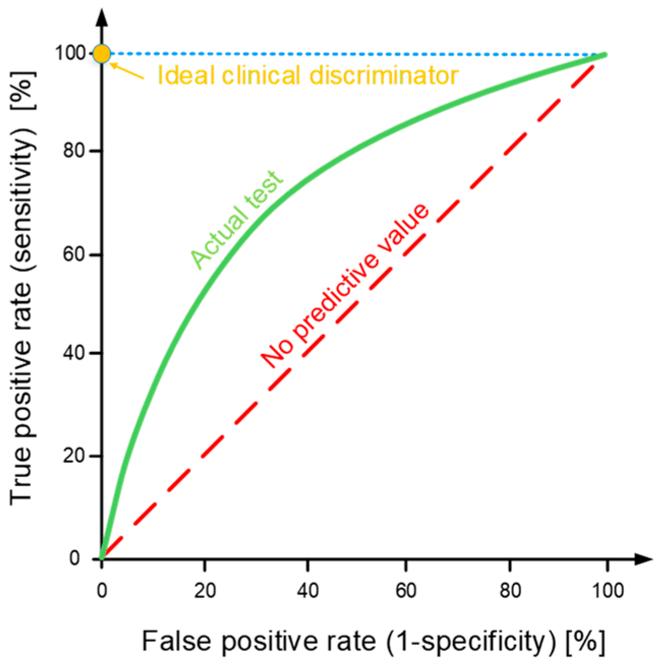
• TPR (true positive rate) and FPR (false positive rate), defined as:

  $$TPR=\frac{TP}{TP+FN}$$

  (1a)

  $$FPR=\frac{FP}{FP+TN}$$

  (1b)

  where: TP (true positive) is the number of true positive events, FN (false negative) is the number of false negative events, FP (false positive) is the number of false positive events, and TN (true negative) is the number of true negative events. TPR and FPR can be visualized by the receiver operating characteristic (ROC) presented in Figure 3, which is often used in comparing pattern recognition algorithms [8]. On the ROC curve, the best detector should be at the position corresponding to TPR = 1 and FPR = 0.
• Precision and Recall: similar to TPR and FPR, precision and recall (sensitivity/sensitiveness) use the values of TP, TN, FP, and FN, and are defined as:

  $$Precision=\frac{TP}{TP+FP}$$

  (2a)

  $$Recall=\frac{TP}{TP+FN}$$

  (2b)
• F-measure (F1 or F-score): the F-measure is the harmonic mean using the definitions of precision and sensitivity and is defined as:

  $$F_{\beta }=\frac{\left({\beta }^2+1\right)·Precision·Recall}{{\beta }^2·Precision+Recall}$$

  (3)

  where a positive factor β determines the influence of the precision and sensitivity values on the F-measure result (β = 1—precision and sensitivity equally important; β < 1—precision more important; β > 1—sensitivity more important).
• Confusion matrix: each element of the confusion matrix represents how often it was confused with other elements of the matrix or how often it was classified correctly.
• Total energy of change: The previous metrics assume that all classification events are equally important, although some devices consume more energy than others. Therefore, considering the weights for each device could help to introduce a parameter to normalize this phenomenon [32].
• Hamming loss: all information lost due to misclassification can be defined by the Hamming loss, which is the ratio of misclassified labels to all labels [58].

2.12. Open Data Sources

To assess the accuracy of the disaggregation algorithms, it is required to use datasets that contain both the total power consumed by all devices connected to the connection and the energy used by individual devices. Below is a list of open datasets that can provide useful data for NILM systems:

• REDD: Reference Energy Disaggregation dataset, containing data from six households, published in 2011, was the first open dataset that could be used to study disaggregation algorithms and at the same time became one of the most widely used for this purpose [59].
• BLUED: The Building Level fully labeled dataset for Electricity Disaggregation was published in [60]. The BLUED dataset contains measured voltage and current data at 12 kHz, collected in one household over a period of one week. Although the dataset does not have data on the electricity use of individual devices, it does contain labels describing exactly when and what devices were activated, which is sufficient for evaluating event-based algorithms.
• Smart*: The Smart* project report published in 2012 [61] includes data from three homes in Massachusetts, USA. Although it does not have data on the use of energy by individual devices in two houses, it does contain data on the temperature and humidity inside the houses and the weather.
• Household Electricity Survey: The Household Electricity Survey is a dataset published in 2012 with data from 251 homes, with 14 of them measured aggregate grid load [62].
• Tracebase: The Tracebase dataset has data from both home and office devices that have been collected using Plugwise devices [63].
• AMPds: The Almanac of Minutely Power dataset was published in [64] and includes data collected in one home over a period of one year. In 2014, the AMPds2 dataset was published, which included data from the following year. The dataset includes measurements of the aggregated load and energy used by individual devices.
• iAWE: Indian data for Ambient Water and Electricity Sensing collected in one home over 73 days was published in [65]. The dataset includes measurements of the aggregated load and energy used by individual devices.
• BERDS: BERkeley EneRgy Disaggregation Dataset contains a set of measurements taken on the UC Berkeley campus, published in [66]. The tested devices include lighting units, pumps, heating, ventilation, and air conditioning. For some of the devices, additional data has been provided in the form of, e.g., air flows.
• ACS-F1: The Appliance Consumption Signatures-Fribourg 1 dataset contains measured electricity consumption data (active power, reactive power, current RMS, phase between voltage and current) collected twice an hour from one hundred household appliances [67].
• UK-DALE: The UK Domestic Appliance-Level Electricity dataset published in [68] includes data from five homes collected over 655 days at 16 kHz for aggregate power and ⅙ Hz for individual appliance power consumption.
• ECO: The Electricity Consumption and Occupancy dataset published in [69] includes data collected from six homes in Switzerland. Data was collected at a sampling frequency of 1 Hz.
• GREEND: The GREEND dataset published in [70] includes data collected from nine homes in Italy. The sampling frequency was 1 Hz.
• SustData: The SustData dataset contains data collected from 50 homes at one-minute intervals [71].
• COMBED: The Commercial Building Energy Dataset contains data from 200 sensors collected on a campus in India at intervals of 30 s [72].
• PLAID: The Plug-Level Appliance Identification Dataset contains 30 kHz rate sampled current and voltage of eleven different household appliances present in fifty-five homes in the United States [73].
• DRED: The Dutch Residential Energy Dataset was published in 2015 and provides information on the energy performance of homes in the Netherlands [74].
• Dataport (Pecan Street): The Dataport Dataset published by Pecan Street Inc. is the largest source of disaggregated energy measurement data in the world, freely available for academic purposes [75]. The database contains data from 722 homes located in Texas, Colorado, and California. The data were collected at one-minute intervals and include the aggregated load and for each device separately.
• OOLL: The Controlled On/Off Loads Library dataset published by the PRISME laboratory of the Université d’Orléans in France contains measurements of current and voltage with a frequency of 100 kHz for forty-two devices belonging to one of twelve classes [76].
• WHITED: The Worldwide Household and Industry Transient Energy Dataset contains start-up data (first five seconds) of one hundred and ten different devices in six different regions around the world, collected at a sampling rate of 44 kHz [77].

The presented list of datasets describes only a certain part of the resources. More appropriate data for a specific experiment can be found in [78].

2.13. Open-Source Tools for NILM

As a result of the growing popularity of disaggregation of energy signals, comparing the disaggregation algorithms proposed by the world of science has become a major challenge. Since many different data sources for NILM have appeared in recent years usually run in a different way, there was a lack of standardized metadata that would allow the use and comparison of these datasets. This is due, among other things, to the fact that many scientists use datasets collected by themselves, as well as there is no standardized set of metrics used by researchers. The lack of standardized performance metrics for disaggregation algorithms motivated the development of the non-intrusive load monitoring toolkit (NILMTK), a toolkit that is used to compare disaggregation algorithms in a reproducible way. NILMTK provides a parser for several existing datasets, a set of pre-processing methods, and a collection of metrics to measure the accuracy of the disaggregation algorithms [58]. In addition, two algorithms have been implemented, combinatorial optimization and HMM, which can be used as a basis for comparisons. In turn, in the study [79], the authors proposed a hierarchical scheme of data recording for energy disaggregation, which create models of devices. This schema was published as an open-source tool and is commonly used by researchers for creating datasets. Since NILMTK was designed with small datasets in mind, in the study [80] the authors proposed the NILMTK v0.2 tool, which enables working with larger datasets by segmenting them and loading them fragmentarily into the computer’s memory. In addition, NILMTK v0.2 offers wider support for several types of metadata contained in datasets.

3. Methodology

In accordance with the assumptions of the project “SESCOM’s Business Intelligence Platform for energy saving and smart facility management”, research on the practical use of NILM in detecting the operation of individual electrical devices in a collective signal was carried out in the form of an experiment.

The experiment was aimed at both verifying the effectiveness of NILM algorithms and checking the usefulness of NILM in commercial telemetry projects, where multi-counter measurement systems would be replaced with a single-counter system and NILM algorithms. For the purposes of this study, a laboratory electrical system with connected devices was designed and built, and then scenarios of interference in the state of these devices were developed, consisting of various times and sequences of switching on and off electrical receivers. The scenarios were performed for many hours in total, and the high frequency sampled signal was stored in a repository on a prepared server.

The analysis of the recorded data was performed using three analytical algorithms: k-nearest neighbors, neural networks, and random forest. The choice of algorithms was based on popularity of algorithms in research on small datasets for machine learning and universality of algorithms for data with different characteristics. In particular, the k-nearest neighbors’ algorithm is considered a low-complexity algorithm, while the random forest is a common method for tabular data with a small number of variables. Neural networks, in turn, work well in the case of games where the values of continuous signals are measured. The operation of the algorithms can be compared by creating a classification report in which various parameters are compiled. The most frequently compared measures include precision (how many of the positively predicted examples are positive), recall (the share of correctly predicted positive cases among all positive cases, including those that were incorrectly classified as negative) and F-measure (the harmonic mean of the precision and recall; the closer to 1, the better classification algorithm).

NILM analytical algorithms have also been validated using BLUED data, commonly used in NILM [78] high-frequency studies (sampling frequency > 1 Hz). BLUED was selected due to the completeness of this set as a set of high-frequency data collected during the measurement of the electrical signal from the building in which approximately 50 electrical energy receivers (devices) were identified. The BLUED set, in addition to voltage and current measurements, has event markers which enables precise identification of the activity of individual devices in the dataset. The use of the BLUED model dataset for NILM disaggregation with the use of the indicated three algorithms is aimed at checking how the results of the data analysis obtained in the experiment coincide with the results of the BLUED data analysis.

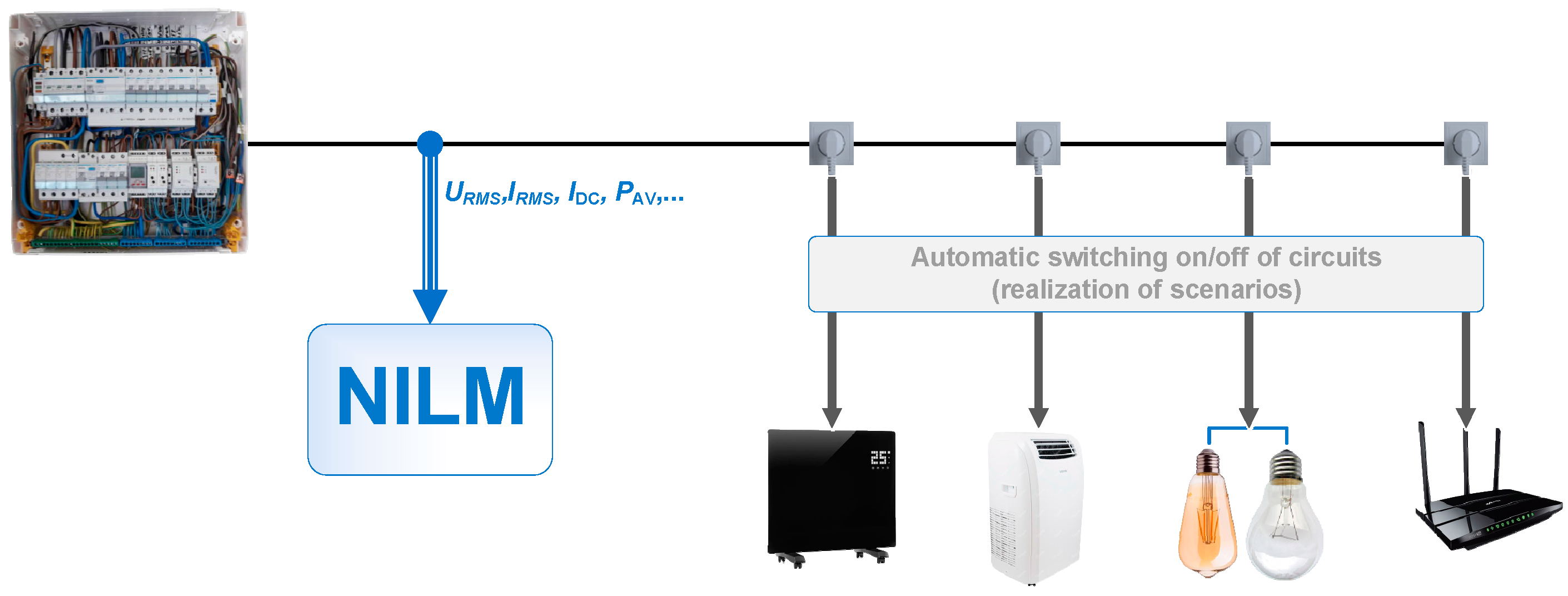
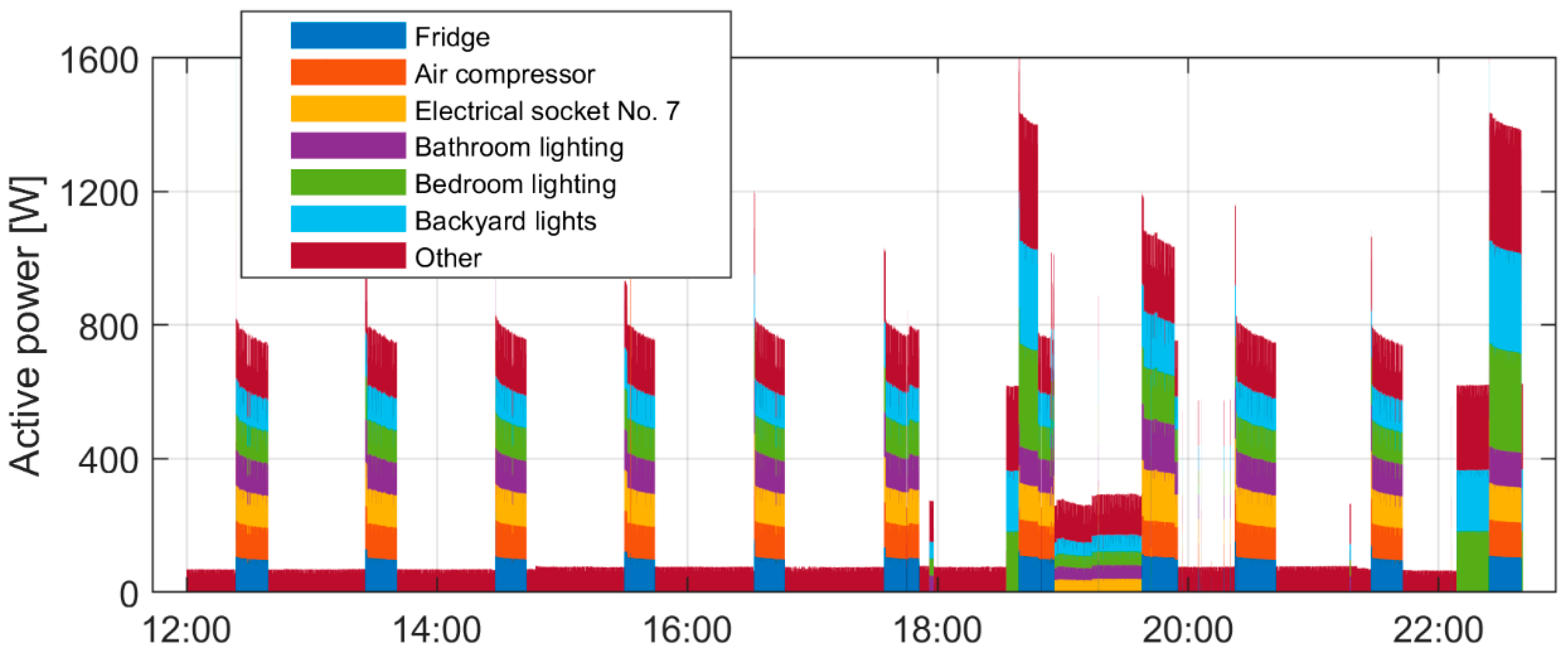
4. Experiment Design

To support our research on a NILM solution, a dataset with requirements was needed. Therefore, the decision was made to pursue the development of a new dataset. The measuring system was equipped with power sockets, which allowed for the simultaneous connection of an air conditioner, two light bulbs (LED and incandescent), a home router, and an electric heater (Figure 4). A synthetic description of the experiment is included in

Table 1. Aggregate information about the experiment.

Element	Description
Loads	Electric heater Air conditioner Two led lamps and one standard incandescent light bulb Home router
Scenarios	Random switching on/off of devices, short intervals between switching on/off the next device ~5–15 s, large differences in device operation time) Units turned on one at a time with a two-minute delay between status changes Devices turned on in pairs with a two-minute delay between status changes Random runs (test sequence).
Measurements	Ih1-10(t)—the amplitudes of the first ten harmonics of the current ih1-10(t)—instantaneous values of the first ten harmonics of the current φh1-10(t)—phase shifts of the first ten harmonics of the current IRMS, IAV, Imax, IDC—current values: rms, average, maximum and DC component respectively

.

The following assumptions were made in preparation for the NILM experiment:

• To implement the experiment scenarios, the devices will be controlled in the given research scenarios by an external controller, implemented using the RaspberryPI microcomputer.
• The non-invasive YHDC AC SCT 013-030 sensor will be used to measure the current,
• Data will be collected by the LabJack U3 chip and stored on the Apache Kafka server. The data will be processed using analytical algorithms selected for the experiment on this server.
• Sampling frequency f = 2 kHz (experimentally determined for the built system).

5. Results Analysis

The set of data (77,742 samples) was collected over a total of 21 h and 25 min. They were divided into a training set (58,306 samples) and a test set (19,436 samples), which contained 75% and 25% of all data from the input set, respectively. The planned scenarios were included in both collections. All experiments assumed a search of hyperparameter values and report the dependence of the results on the values corresponding to individual hyperparameter models, thereby enabling the best configuration of a given model to be found. The measurement results were analyzed using three implemented methods:

• k-Nearest Neighbors,
• Neural Networks,
• Random Forest.

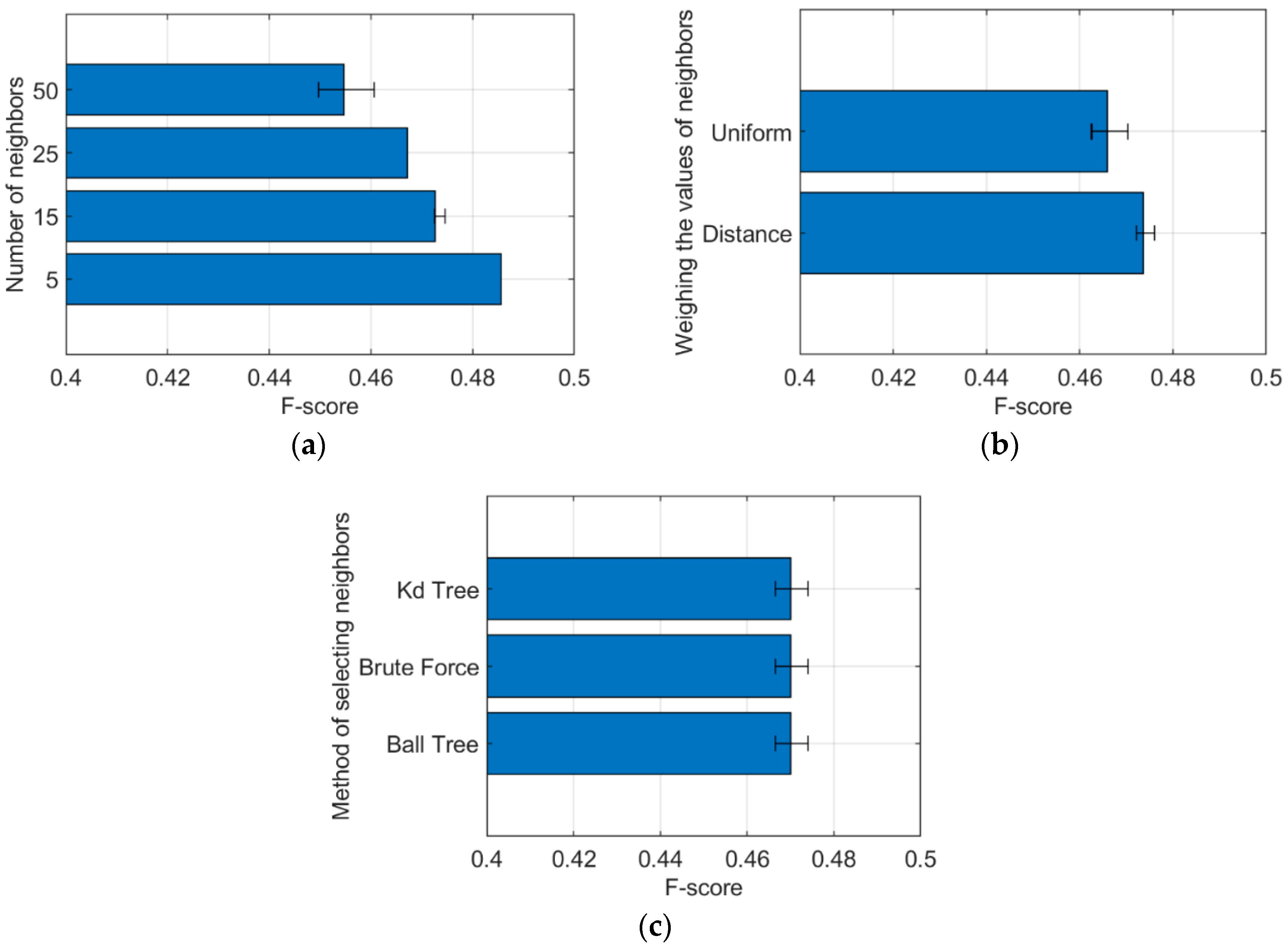
5.1. k-Nearest Neighbors (k-NN)

The k-NN classification approach presented below aims to assign each example to a possible combination of device states (which are assumed to be binary, corresponding to the status of the switch).

With the increase in the number of nearest neighbors considered when determining the status of the device, the value of the F-measure decreased, and the best results were obtained for 5 neighbors (Figure 5a and Figure 5b, respectively). The influence of the method of selecting the nearest neighbors did not affect the correctness of the classification (Figure 5c). The drawings in the Figure 5 contain the so-called 95% confidence interval (black sections on the measurement bars), which (in this case) is of negligible importance in the interpretation of the results.

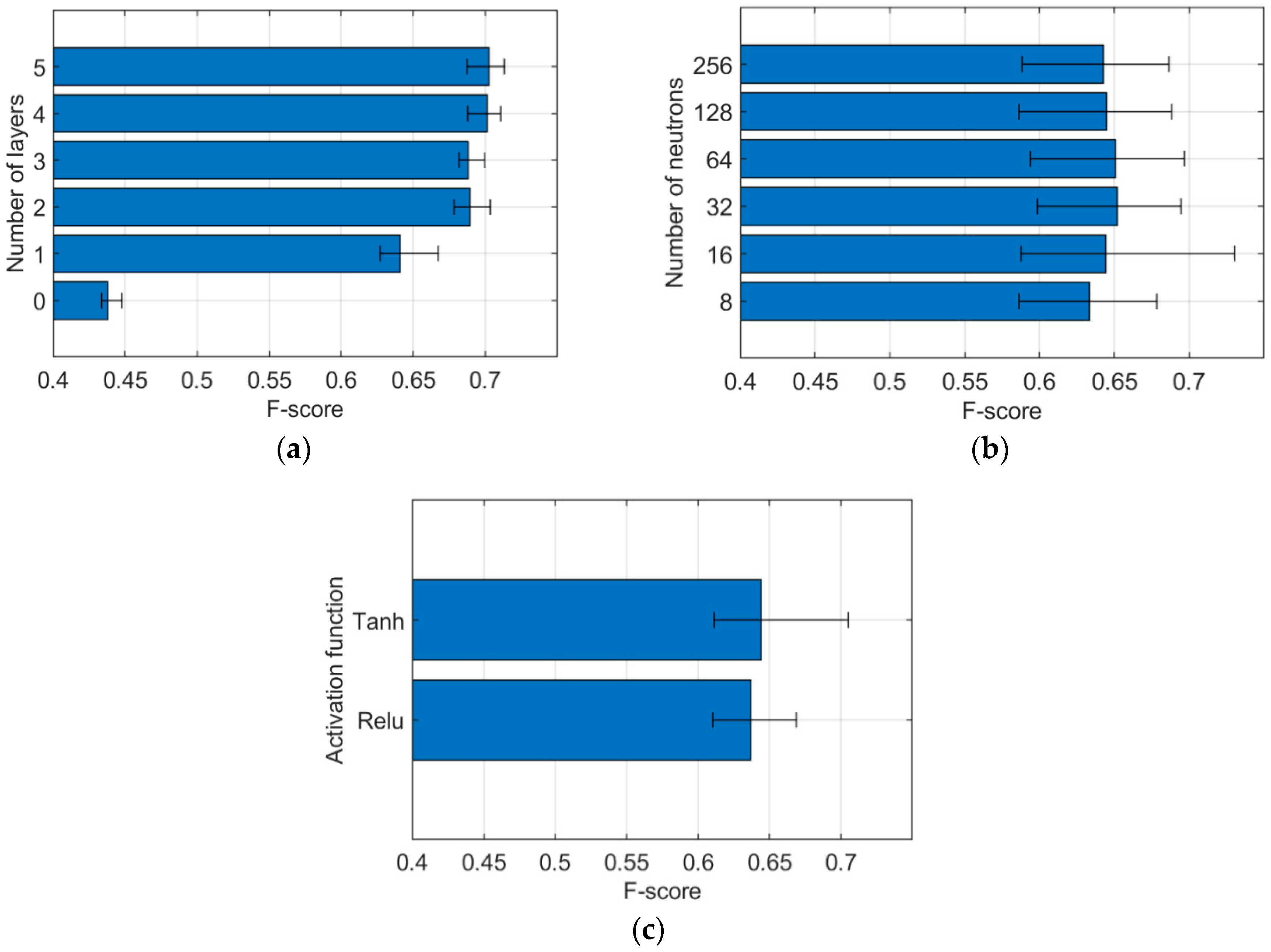
5.2. Neural Networks

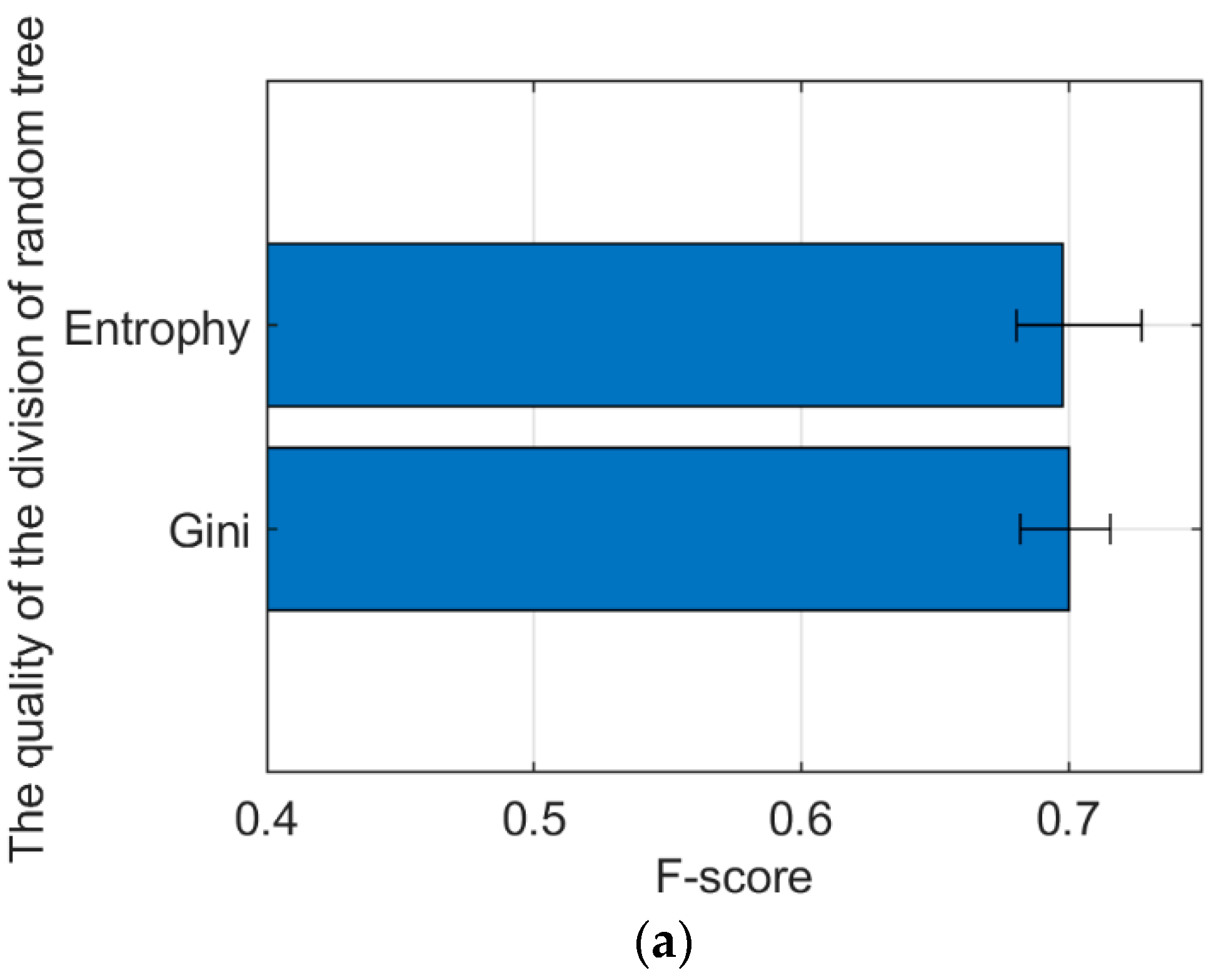
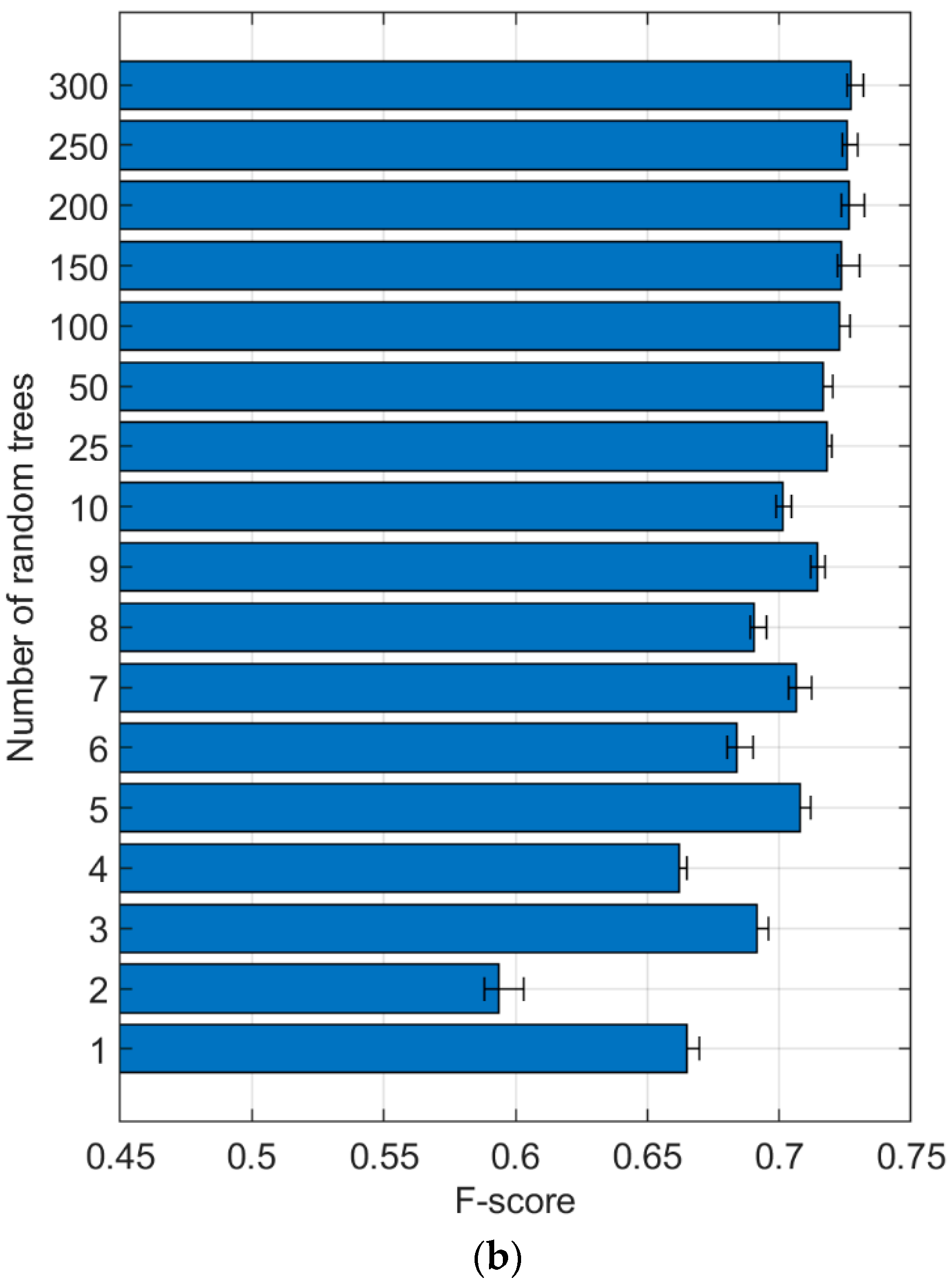
The neural network was adopted as structure with a different number of fully connected layers (called hidden layers) and with a different number of neurons in them (the number of neurons determines the size of the layer). For each model, the last layer of the network, which consisted of four neurons, was identical, followed by a sigmoidal activation function. Subsequent models differed in the number of hidden layers and their size. After each layer, one of two activation functions was selected: ReLU (rectifier linear unit) or hyperbolic tangent (tanh).

The Adam optimizer was selected as the model weight selection algorithm. The highest accuracy value was achieved for two hidden layers (Figure 6a). Figure 6b shows that the optimal number of neurons in the hidden layers should be in the range of 32–64. The hyperbolic tangent as an activation function in the part of the network responsible for feature extraction had a slightly better classification accuracy than the ReLU function (Figure 6c).

5.3. Random Forest

The values of two important hyperparameters were tested: the collection impurity measure and the number of trees in the classifier. The two measures of impurity of a set available for a classification problem are entropy and the Gini index.

Larger values of the F-measure were obtained using entropy than the Gini index (Figure 7a). On the other hand, from the number of 150 trees, the correctness remained at a similar level (Figure 7b), from which it can be concluded that this number of trees is sufficient for this problem.

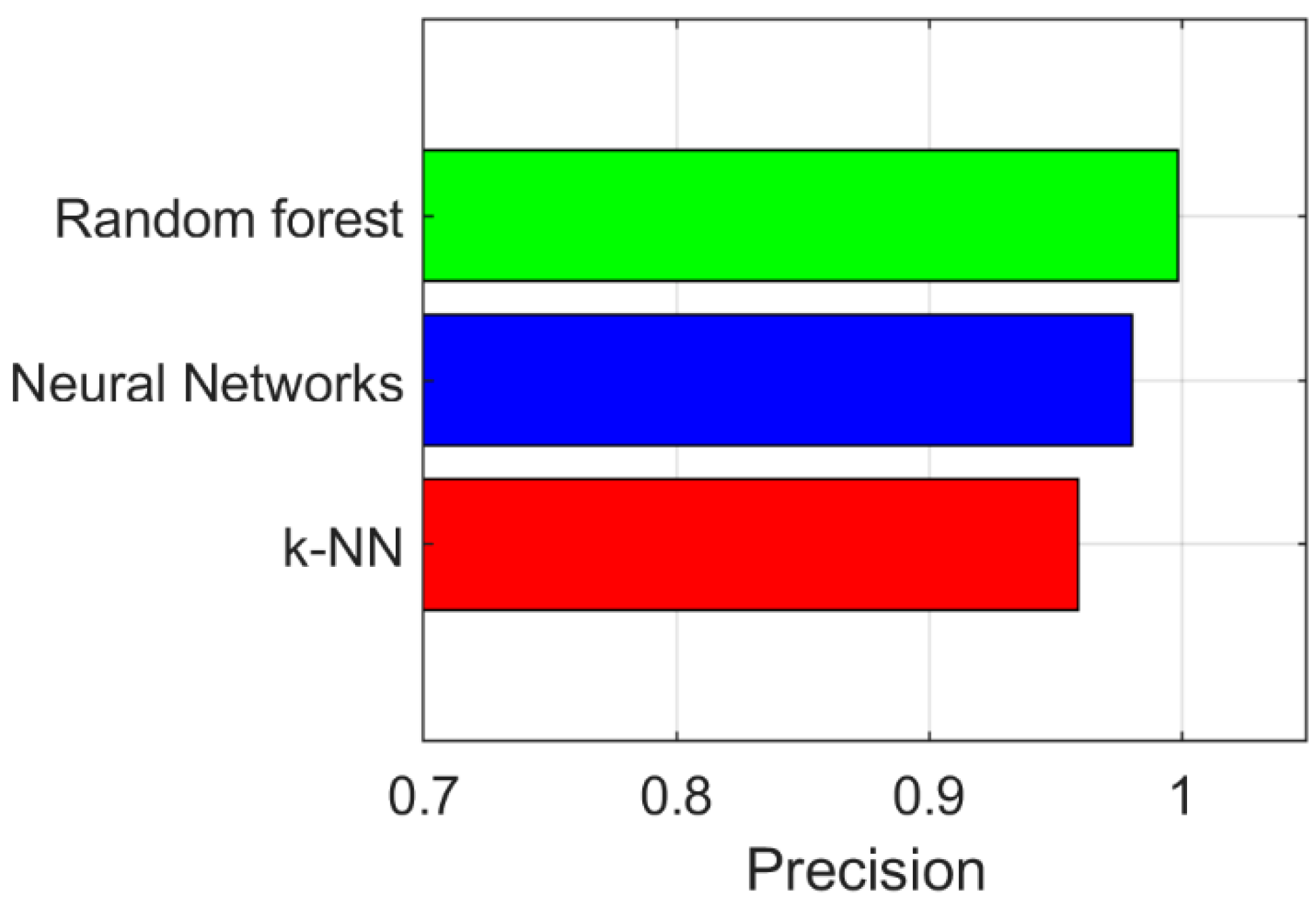
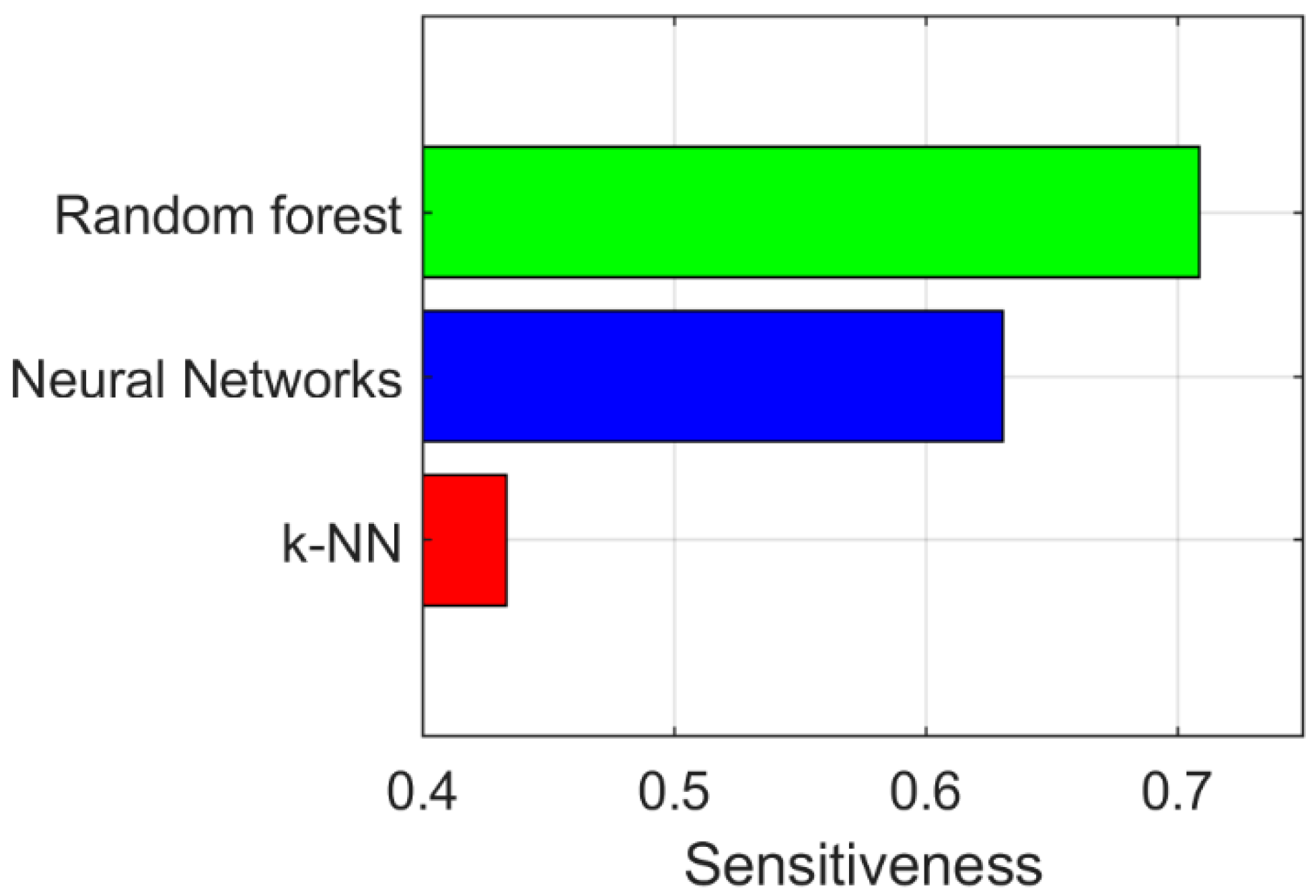
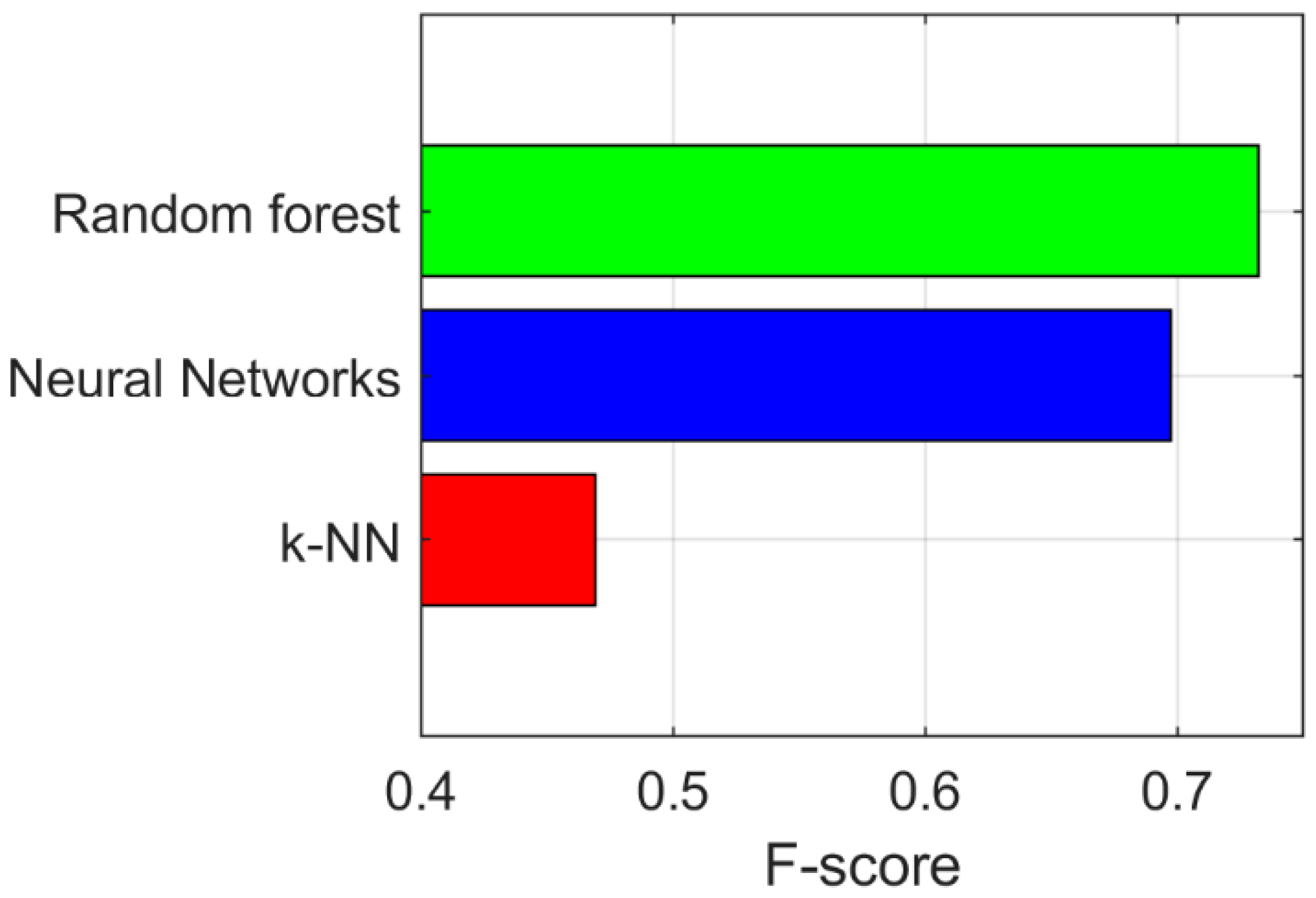
5.4. Comparison of Methods

For the sensitivity and F-measure metrics, random forest is by far the best algorithm, whereas neural networks were characterized by the highest precision, and the k-nearest neighbors algorithm was by far the worst (Figure 8, Figure 9 and Figure 10).

The correctness of the classification of individual devices connected to the electrical network was also checked. In the test set, the condition of the air conditioner and light bulb were correctly classified with a high precision of about 85%, while worse results were obtained for the router with a precision of nearly 70%. The worst results were obtained for the resistive electric heater with precision close to 60%, which is only slightly better than randomly guessing the device status. An electric heater is characterized by rare changes of on/off status, and such a constant characteristic makes it difficult to analyze the presence of this element in the system.

Based on the data in the figures above, it can be concluded that random forest turned out to be the best among the tested algorithms. For the sensitivity and F-measure metrics, random forest is by far the best algorithm. On the other hand, neural networks were characterized by the highest precision, and the k-nearest neighbors algorithm fared the worst. The correctness of the classification of individual devices connected to the electrical network was also checked.

In the test set, the condition of the air conditioner and light bulb were correctly classified with a high precision of about 85%, while worse results were obtained for the router with a precision of nearly 70% (Figure 11). By far, the worst results were obtained for the electric heater, which scored close to 60% (Figure 11), which is a result close to that which could be obtained by randomly guessing the device status.

Results obtained for the electric heater can be improved. A larger number of measurement samples would be required to record more changes in the heater’s on/off state. Additionally, by installing among others the temperature sensor in the heater’s vicinity, additional variable can be added (heater’s ambient temperature) to correlate the temperature sensor’s indications with changes in the heater’s operating status in the electrical collective signal. Moreover, such attempts will be made by the authors in the near future. The authors expect then a significant increase in the effectiveness of learning. However, it should be remembered that commercial solutions must be economically justified, so the conducted research will focus on identifying a solution that allows for a compromise between the increase in learning efficiency and the expenditure on the expansion of measurement systems.

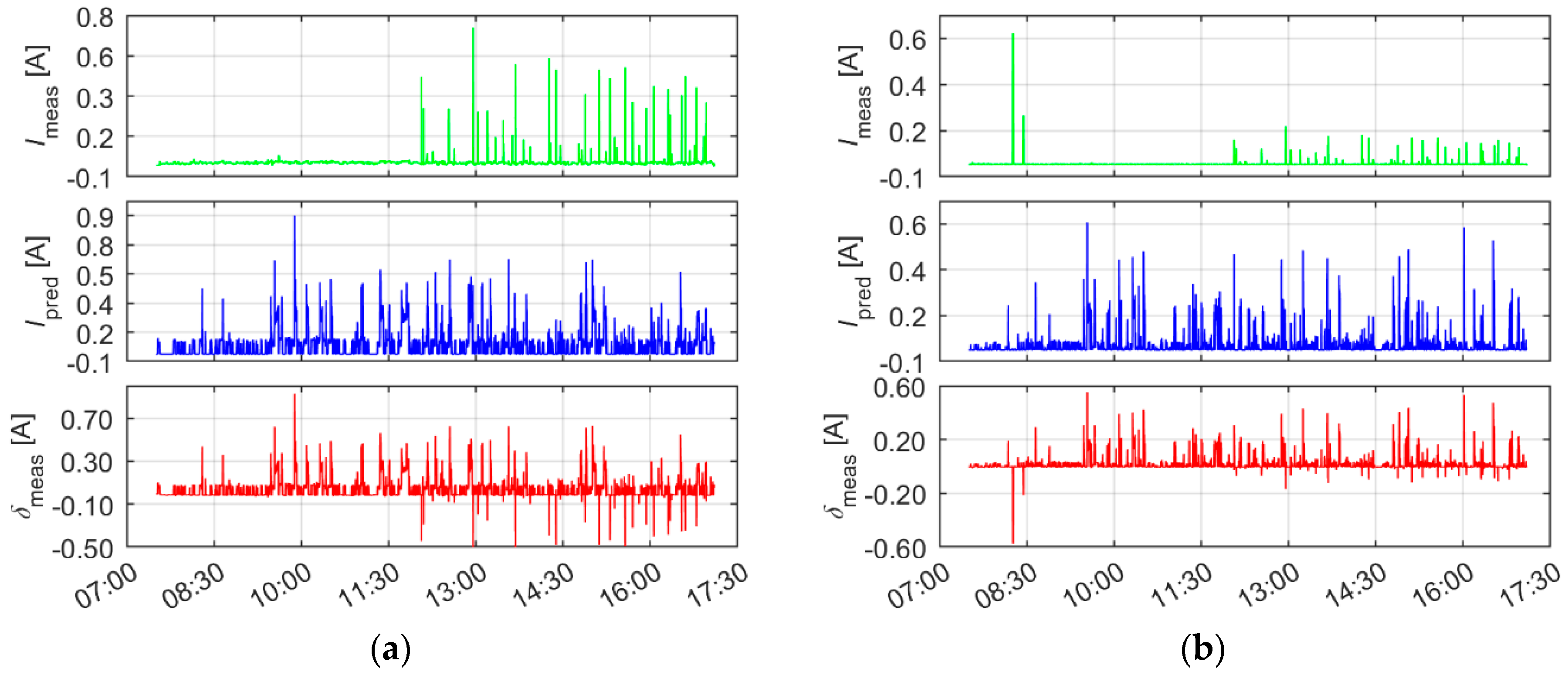
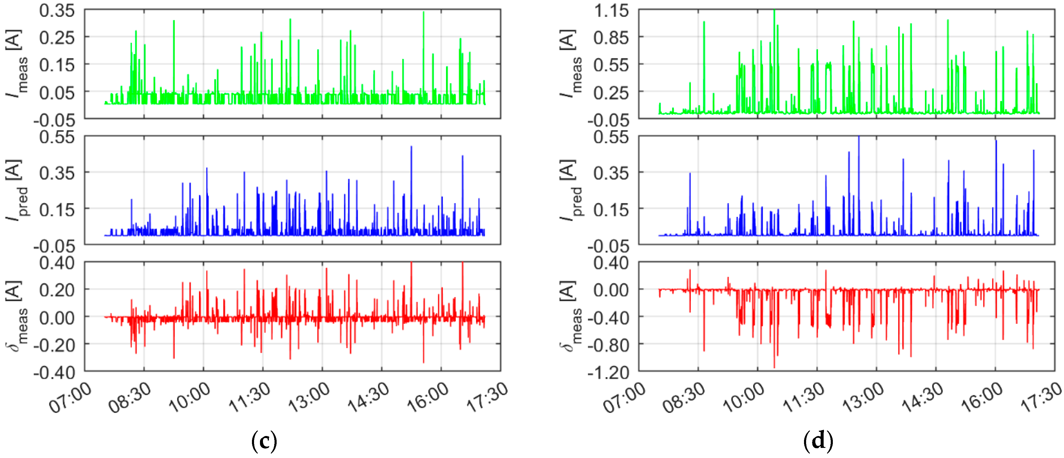
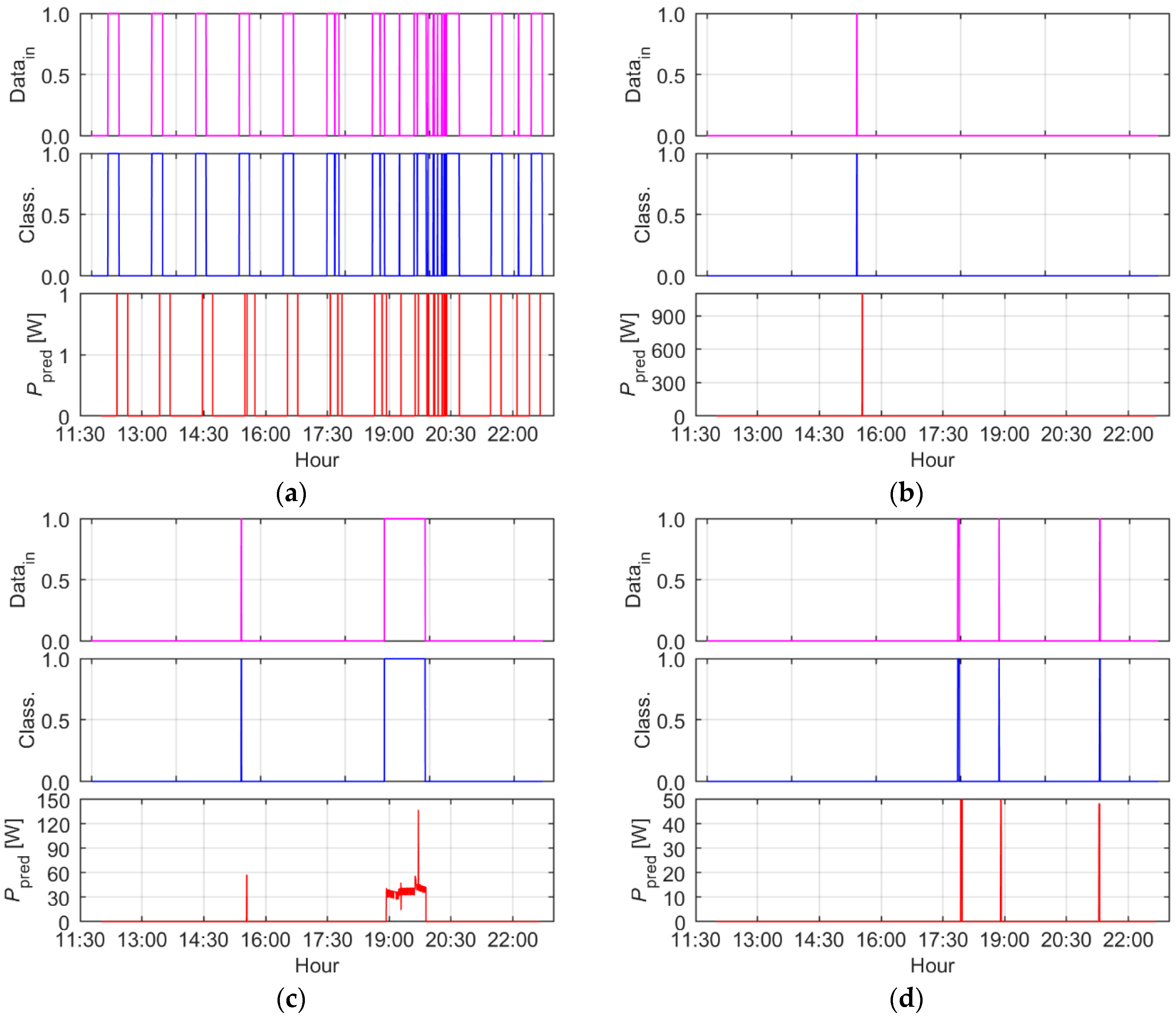
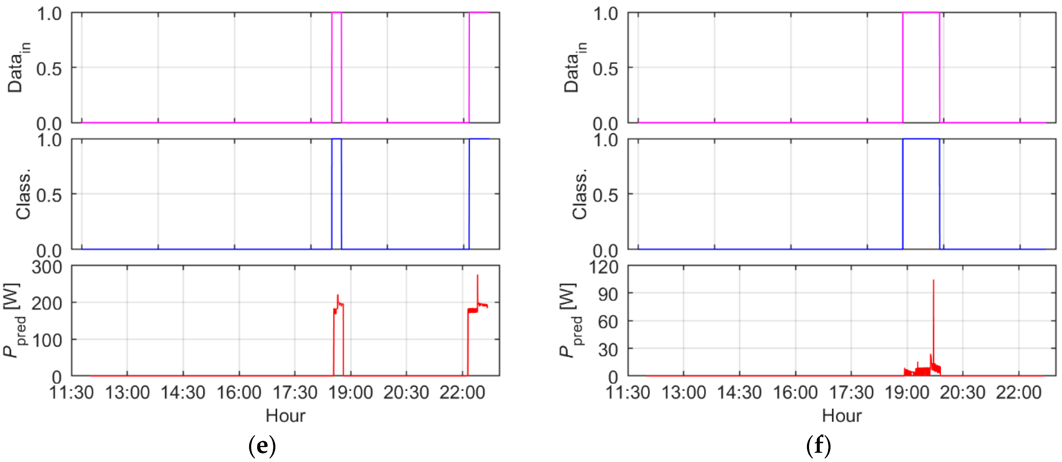
5.5. Prediction of Power Consumed by Devices

Based on the classification results for the entire dataset, the predicted power consumed by individual devices was also determined. The first step was to calculate the average power of each device ${\overline{p}}_i$ by minimizing expression (4), where T is the number of time samples, D the number of devices, $P_t$ the total power at time t, and $a_{i,t}$ the binary variable specifying whether the i-device is active at time t, where i denotes device index.

$$\underset{{\overline{p}}_i}{\min }{\displaystyle \sum }_{t=1}^T{\left(P_t-{\displaystyle \sum }_{i=1}^D{a}_{i,t}{\overline{p}}_i\right)}^2$$

(4)

Knowing the predicted average power of each device, the instantaneous power was also determined. It was assumed that the determined average power of the device ${\overline{p}}_i$ was the more precisely determined the greater number of samples $n_i$ for i-device was utilized. It was assumed that the power consumption by a device is a stationary process. Therefore, the instantaneous power should be closer to the average power estimate with a greater number of samples utilized. At each moment of time, the value $e_t$ was determined (5), i.e., the difference between the actual power in the network and the sum of the average power values of the connected devices:

$$e_t=P_t-{\displaystyle \sum }_{i=1}^D{a}_{i,t}{\overline{p}}_i$$

(5)

Factor $N_t$ was specified, as the sum of $n_i$ factors of the devices turned on at the moment of time t:

$$N_t={\displaystyle \sum }_{i=1}^D{a}_{i,t}{n}_i$$

(6)

The instantaneous power $p_{i,t}$ of the device at the moment t of time was determined as the sum of the estimated value of the average power ${\overline{p}}_i$ of the device and the value $e_t$ properly scaled so that larger values were added to devices for which fewer measurements were available.

$$p_{i,t}={\overline{p}}_i+e_t\frac{N_t-n_i}{S_t{{\displaystyle \sum }}_i^D{a}_{i,t}}$$

(7)

Due to the low precision of the classification of the operating status of the device, the above-described method of predicting the power or current (Figure 12) consumption of the device was burdened with a large error. The biggest problem was the heater (Figure 13d), which according to the measurements was characterized by the highest power consumption and was at the same time classified the worst, which translated directly into the current prediction error of this device, sometimes reaching 1 A, as well as into the error of the others, where for the air conditioner and the router it reached 0.5 A (Figure 13a,b). For bulbs with maximum errors, it was approximately 0.25 A (Figure 13c). Also puzzling are the numerous, large, temporary spikes in current consumption, which may be due to measurement errors.

Each misclassification has a variable effect on power measurements and devices that operate infrequently and have relatively low power (compared to other devices in the system) are most vulnerable to the negative impact of errors. In this case, classifying a long-running device (as a device that typically only runs briefly) can significantly increase reported energy consumption. The use of additional heuristics or statistical analysis could help to reject some of the incorrect classifications by analyzing the power used, e.g., in the case of classifying devices that typically use low power (e.g., 2 kW) as high power devices (e.g., 10 kW) or analyzing the length of time the device is switched on and the continuity of its operation.

The obtained results and changes in settings made during the experiments confirmed that the values of algorithm quality indicators (precision 0.756, sensitivity 0.708, F-measure 0.731) achieved by random forest confirm that devices are identified with an average of approximately 75% correctness, which is a satisfying result, however still requiring improvement in commercial applications. The limitation of the optimization of the operation of algorithms is the sampling frequency, which in the experiments described in other publications reaches up to 12 kHz (in described in the paper experiment, the maximum sampling frequency is 2 kHz, the increase of this frequency resulted in incomplete data). The limitation was the LAB JACK sampling system. Moreover, due to the separation of the measurement system and the system responsible for controlling the process of switching on and off devices, there was a problem with the synchronization of measurements, which also had an impact on the deterioration of the results. The conclusion is that after eliminating the above-mentioned problems and increasing the sampling frequency, the classification results are expected to improve.

6. BLUED Data Analysis

Power measurements of individual devices were not available for BLUED data. Quantitative analysis, correct determination of the instantaneous power of devices, and determination of the exact prediction error were not possible. However, it can be noticed that, for a refrigerator, the assumption of stationarity of the power function is most likely incorrect and the power consumed by it decreases with time after switching it on (Figure 14). Figure 15 shows the prediction of the moment of switching on the devices, along with the actual switching-on time and the prediction of the power consumed by them.

Each misclassification has a different effect on power measurements. The most vulnerable to the negative impact of errors are devices that operate infrequently and have relatively low power compared to other devices. In this case, classifying a long-running device (as a device that typically only runs briefly) can significantly increase reported energy consumption. It is worth noting that the use of additional heuristics or statistical analysis could help to reject some incorrect classifications by analyzing the power consumed, e.g., in the case of classifying devices that usually consume low power (e.g., 2 kW) as devices that consume high power (e.g., 10 kW), or by analysis of the length of activation of the device and the continuity of its operation.

7. Conclusions, Implications, Limitations, and Future Work

7.1. Research Conclusions

Analyzing aggregated power consumption data is still a challenging problem. ILM systems provide high accuracy but are expensive, space constraints and complicated because energy consumption is measured by installing a meter on each individual load. In NILM systems, energy consumption is measured at the MPI and individual contributions relating to each load are obtained by “disaggregating” signal. As part of the research, an experimental electrical system was designed. Connected electrical devices were switched on and off according to developed scenarios. During the measurements, the electrical collective signal was sampled with the LAB JACK system, and the obtained data were saved on the server. The sampling frequency was set to 2 kHz, which ensured the correct saving of all samples on the server. The obtained data were verified using MLA, of which the random forest turned out to be the best. A summary of individual indicators for the compared methods is shown in the Figure 16.

To verify the quality of the performed experiment, selected analytical algorithms were used similarly for the disaggregation of the BLUED data. As presented in this paper, research aiming to disaggregate the electrical collective signal MLA was used. Although the obtained accuracy of device detection did not improve the results described in the literature so far (e.g., [81,82]), the use of machine learning algorithms confirms the legitimacy of their use in NILM research.

7.2. Implications for Theory and Practice

The results of disaggregation and the developed conclusions have implications both in theory and practice of using NILM in the decomposition of an electrical signal. Regarding the research conducted in the past using various disaggregation techniques [12,82,83], the experiment confirmed the possibility of using k-NN machine learning algorithms, random forest, and neural networks for NILM. The article indicates the metrics that selected random forest from among the tested algorithms, enabling signal disaggregation with the highest probability of correct detection of single signals from electrical devices. An additional contribution to the theory is the dataset generated in the experiment, which, together with the documentation regarding the measurement system and data format, was made available free of charge to other researchers [84]. Thus, another laboratory developed NILM dataset was created, which extends the database of existing datasets used by researchers to carry out their own research.

Research results also offer a set of practical remarks for the managerial staff, engineers, and experts from the energy efficiency industry, who see NILM technologies as an opportunity to decompose electrical signals using analytical algorithms and effectively manage electricity consumption. Of great interest are the economic benefits of the NILM method using the measurement at the MP, replacing the system with individual measurement of loads and thus reducing the costs of installation and operation of individual meters. The review of the literature and the experiment confirmed that the MLA enable determining the structure of the collective signal components composed of the signals of individual devices, but the isolation accuracy is unsatisfactory to use the method commercially. It is not possible to make the right decisions regarding the consumption of electricity by circuits or devices when there is not close to 100% certainty about the correctness of the isolation of component signals within the collective signal. The NILM gives some clues and a general idea of what is in the electrical collective signal. The knowledge acquired in NILM can be used to describe the general population and operation of devices, which probably opens low-cost possibilities for performing preliminary analyses without the need to install complex multi-counter measurement systems. If NILM demonstrates that there is a significant potential for saving electricity in a building electrical circuit, then taking further steps (including investment) in energy efficiency management projects will no longer be just a theoretical assumption, but a real analytical result based on NILM.

7.3. Limitations and Potential Future Research Directions

The potential and benefit of NILM service are known, but its real-world deployment has been still limited. The results of the correctness of signal detection obtained in the research did not lead the authors of this article to develop an NILM method which would give 100% certainty of the correctness of disaggregation. The obtained results correspond to the results of research works described numerously in the literature [85,86]. The main limitations of the experiment include the sampling frequency of 2 kHz, the increase of which could improve the results of disaggregation. Another limitation was the too short duration of the experiment, as more measurement data enable better training of analytical algorithms. The computational complexity of tested algorithms was also not assessed, which may be significant when processing large volumes of data [87].

An effort in future works will be directed towards answering the question: under what conditions will the NILM analysis, burdened with a certain error, enable effective management of the energy efficiency of buildings? Additionally, as part of our future work, we intend to evaluate FDII (fault detection, identification, and isolation) and PDM (predictive maintenance) technologies, which areas important for the effective and economical management of building facilities.

References

1. Gawin, B.; Marcinkowski, B. Setting up Energy Efficiency Management in Companies: Preliminary Lessons Learned from the Petroleum Industry. Energies 2020, 13, 5604. [Google Scholar] [CrossRef]
2. Mahi-al-rashid, A.; Hossain, F.; Anwar, A.; Azam, S. False Data Injection Attack Detection in Smart Grid Using Energy Consumption Forecasting. Energies 2022, 15, 4877. [Google Scholar] [CrossRef]
3. Puente, C.; Palacios, R.; González-Arechavala, Y.; Sánchez-Úbeda, E.F. Non-Intrusive Load Monitoring (NILM) for Energy Disaggregation Using Soft Computing Techniques. Energies 2020, 13, 3117. [Google Scholar] [CrossRef]
4. Rafati, A.; Shaker, H.R.; Ghahghahzadeh, S. Fault Detection and Efficiency Assessment for HVAC Systems Using Non-Intrusive Load Monitoring: A Review. Energies 2022, 15, 341. [Google Scholar] [CrossRef]
5. Shin, C.; Rho, S.; Lee, H.; Rhee, W. Data Requirements for Applying Machine Learning to Energy Disaggregation. Energies 2019, 12, 1696. [Google Scholar] [CrossRef] [Green Version]
6. Mari, S.; Bucci, G.; Ciancetta, F.; Fiorucci, E.; Fioravanti, A. A Review of Non-Intrusive Load Monitoring Applications in Industrial and Residential Contexts. Energies 2022, 15, 9011. [Google Scholar] [CrossRef]
7. Fotopoulou, M.; Petridis, S.; Karachalios, I.; Rakopoulos, D. A Review on Distribution System State Estimation Algorithms. Appl. Sci. 2022, 12, 11073. [Google Scholar] [CrossRef]
8. Zoha, A.; Gluhak, A.; Imran, M.; Rajasegarar, S. Non-Intrusive Load Monitoring Approaches for Disaggregated Energy Sensing: A Survey. Sensors 2012, 12, 16838–16866. [Google Scholar] [CrossRef] [Green Version]
9. Hart, G.W. Nonintrusive appliance load monitoring. Proc. IEEE 1992, 80, 1870–1891. [Google Scholar] [CrossRef]
10. Yu, J.; Gao, Y.; Wu, Y.; Jiao, D.; Su, C.; Wu, X. Non-Intrusive Load Disaggregation by Linear Classifier Group Considering Multi-Feature Integration. Appl. Sci. 2019, 9, 3558. [Google Scholar] [CrossRef] [Green Version]
11. Laouali, I.; Gomes, I.; da Ruano, M.G.; Bennani, S.D.; El Fadili, H.; Ruano, A. Energy Disaggregation Using Multi-Objective Genetic Algorithm Designed Neural Networks. Energies 2022, 15, 9073. [Google Scholar] [CrossRef]
12. Biansoongnern, S.; Plungklang, B. Non-Intrusive Appliances Load Monitoring (NILM) for Energy Conservation in Household with Low Sampling Rate. Procedia Comput. Sci. 2016, 86, 172–175. [Google Scholar] [CrossRef] [Green Version]
13. Chrysostomou, G.; Shikhin, V.; Shikhina, A. Electrical Energy Supply Control Support via Meters Data Ellipsoidal Approximation in Smart Grids. Procedia Comput. Sci. 2017, 103, 287–294. [Google Scholar] [CrossRef]
14. Norford, L.K.; Leeb, S.B. Non-intrusive electrical load monitoring in commercial buildings based on steady-state and transient load-detection algorithms. Energy Build. 1996, 24, 51–64. [Google Scholar] [CrossRef]
15. Laughman, C.; Lee, K.; Cox, R.; Shaw, S.; Leeb, S.; Norford, L.; Armstrong, P. Power signature analysis. IEEE Power Energy Mag. 2003, 1, 56–63. [Google Scholar] [CrossRef]
16. Chang, H.-H.; Yang, H.-T.; Lin, C.-L. Load Identification in Neural Networks for a Non-intrusive Monitoring of Industrial Electrical Loads. In Computer Supported Cooperative Work in Design IV; Shen, W., Yong, J., Yang, Y., Barthès, J.-P.A., Luo, J., Eds.; Springer: Berlin/Heidelberg, Germany, 2008; pp. 664–674. [Google Scholar]
17. Gupta, S.; Reynolds, M.S.; Patel, S.N. ElectriSense. In Proceedings of the 12th ACM International Conference on Ubiquitous Computing, Pittsburgh, PA, USA, 26–29 September 2010; ACM: New York, NY, USA, 2010; pp. 139–148. [Google Scholar]
18. Berenguer, M.; Giordani, M.; Giraud-By, F.; Noury, N. Automatic detection of activities of daily living from detecting and classifying electrical events on the residential power line. In Proceedings of the HealthCom 2008-10th International Conference on e-health Networking, Applications and Services, Singapore, 7–9 July 2008; pp. 29–32. [Google Scholar]
19. Najafi, B.; Moaveninejad, S.; Rinaldi, F. Data Analytics for Energy Disaggregation: Methods and Applications. In Big Data Application in Power Systems; Elsevier: Amsterdam, The Netherlands, 2018; pp. 377–408. [Google Scholar]
20. Patel, S.N.; Robertson, T.; Kientz, J.A.; Reynolds, M.S.; Abowd, G.D. At the Flick of a Switch: Detecting and Classifying Unique Electrical Events on the Residential Power Line (Nominated for the Best Paper Award). In UbiComp 2007: Ubiquitous Computing; Krumm, J., Abowd, G.D., Seneviratne, A., Strang, T., Eds.; Springer: Berlin/Heidelberg, Germany, 2007; pp. 271–288. [Google Scholar]
21. Drenker, S.; Kader, A. Nonintrusive monitoring of electric loads. IEEE Comput. Appl. Power 1999, 12, 47–51. [Google Scholar] [CrossRef]
22. Cole, A.I.; Albicki, A. Algorithm for nonintrusive identification of residential appliances. In Proceedings of the1998 IEEE International Symposium on Circuits and Systems (ISCAS), Monterey, CA, USA, 31 May–3 June 1998; Volume 3, pp. 338–341. [Google Scholar]
23. Cole, A.I.; Albicki, A. Data extraction for effective non-intrusive identification of residential power loads. In Proceedings of the IMTC/98 Conference Proceedings. IEEE Instrumentation and Measurement Technology Conference. Where Instrumentation Is Going (Cat. No. 98CH36222), St. Paul, MN, USA, 18–21 May 1998; Volume 2, pp. 812–815. [Google Scholar]
24. Liang, J.; Ng, S.K.K.; Kendall, G.; Cheng, J.W.M. Load Signature Study—2014; Part I: Basic Concept, Structure, and Methodology. IEEE Trans. Power Deliv. 2010, 25, 551–560. [Google Scholar] [CrossRef]
25. Leeb, S.B.; Shaw, S.R.; Kirtley, J.L. Transient event detection in spectral envelope estimates for nonintrusive load monitoring. IEEE Trans. Power Deliv. 1995, 10, 1200–1210. [Google Scholar] [CrossRef] [Green Version]
26. Lee, W.Y.; Lee, Y.C.; Sokolov, K.; Lee, H.J.; Moon, I. LED projection displays. In Nonimaging Optics and Efficient Illumination Systems; Winston, R., Koshel, R.J., Eds.; SPIE: Denver, CO, USA, 2004; Volume 5529, pp. 1–7. [Google Scholar]
27. Lam, H.; Fung, G.; Lee, W. A Novel Method to Construct Taxonomy Electrical Appliances Based on Load Signaturesof. IEEE Trans. Consum. Electron. 2007, 53, 653–660. [Google Scholar] [CrossRef] [Green Version]
28. Zeifman, M.; Roth, K. Nonintrusive appliance load monitoring: Review and outlook. IEEE Trans. Consum. Electron. 2011, 57, 76–84. [Google Scholar] [CrossRef]
29. Dong, M.; Meira, P.C.; Xu, W.; Chung, C.Y. Non-Intrusive Signature Extraction for Major Residential Loads. IEEE Trans. Smart Grid 2013, 4, 1421–1430. [Google Scholar] [CrossRef] [Green Version]
30. Abubakar, I.; Khalid, S.N.; Mustafa, M.W.; Shareef, H.; Mustapha, M. Application of load monitoring in appliances’ energy management—A review. Renew. Sustain. Energy Rev. 2017, 67, 235–245. [Google Scholar] [CrossRef]
31. Kolter, J.; Batra, S.; Ng, A. Energy Disaggregation via Discriminative Sparse Coding. Adv. Neural Inf. Process. Syst. 2010, 23, 1153–1161. [Google Scholar]
32. Anderson, K.D. Non-Intrusive Load Monitoring: Disaggregation of Energy by Unsupervised Power Consumption Clustering. Ph.D. Thesis, Carnegie Mellon University, Pittsburgh, PA, USA, 2014. [Google Scholar]
33. Hart, G.W.; Kern, E.C.J.; Schweppe, F.C. Non-intrusive Appliance Monitor Apparatus. U.S. Patent 4858141, 15 August 1989. [Google Scholar]
34. Du, Z.; Li, J.; Zhu, L.; Lu, K.; Shen, H.T. Adversarial Energy Disaggregation. ACM/IMS Trans. Data Sci. 2021, 2, 1–16. [Google Scholar] [CrossRef]
35. Kelly, J.; Knottenbelt, W. Neural NILM: Deep Neural Networks Applied to Energy Disaggregation. arXiv 2015, arXiv:1507.06594. [Google Scholar]
36. Zhang, C.; Zhong, M.; Wang, Z.; Goddard, N.; Sutton, C. Sequence-to-Point Learning With Neural Networks for Non-Intrusive Load Monitoring. In Proceedings of the Thirty-Second AAAI Conference on Artificial Intelligence (AAAI-18), New Orleans, LO, USA, 2–7 February 2018; Volume 32. [Google Scholar] [CrossRef]
37. Pan, Y.; Liu, K.; Shen, Z.; Cai, X.; Jia, Z. Sequence-To-Subsequence Learning With Conditional Gan For Power Disaggregation. In Proceedings of the ICASSP 2020—2020 IEEE International Conference on Acoustics, Speech and Signal Processing (ICASSP), Barcelona, Spain, 4–8 May 2020; pp. 3202–3206. [Google Scholar]
38. Leeb, S.B.; Kirtley, J.L. A Conjoint Pattern Recognition Approach to Nonintrusive Load Monitoring; Massachusetts Institute of Technology: Cambridge, MA, USA, 1993. [Google Scholar]
39. Farinaccio, L.; Zmeureanu, R. Using a pattern recognition approach to disaggregate the total electricity consumption in a house into the major end-uses. Energy Build 1999, 30, 245–259. [Google Scholar] [CrossRef]
40. Marchiori, A.; Hakkarinen, D.; Han, Q.; Earle, L. Circuit-Level Load Monitoring for Household Energy Management. IEEE Pervasive Comput. 2011, 10, 40–48. [Google Scholar] [CrossRef]
41. Srinivasan, D.; Ng, W.S.; Liew, A.C. Neural-Network-Based Signature Recognition for Harmonic Source Identification. IEEE Trans. Power Deliv. 2006, 21, 398–405. [Google Scholar] [CrossRef]
42. Ruzzelli, A.G.; Nicolas, C.; Schoofs, A.; O’Hare, G.M.P. Real-Time Recognition and Profiling of Appliances through a Single Electricity Sensor. In Proceedings of the 7th Annual IEEE Communications Society Conference on Sensor, Mesh and Ad Hoc Communications and Networks, Boston, MA, USA, 21–25 June 2010; pp. 1–9. [Google Scholar]
43. Zia, T.; Bruckner, D.; Zaidi, A. A hidden Markov model based procedure for identifying household electric loads. In Proceedings of the 37th Annual Conference of the IEEE Industrial Electronics Society (IECON 2011), Melbourne, VIC, Australia, 7–10 November 2011; pp. 3218–3223. [Google Scholar]
44. Figueiredo, M.B.; de Almeida, A.; Ribeiro, B. An Experimental Study on Electrical Signature Identification of Non-Intrusive Load Monitoring (NILM) Systems. In Adaptive and Natural Computing Algorithms; Dobnikar, A., Lotrič, U., Šter, B., Eds.; Springer: Berlin/Heidelberg, Germany, 2011; pp. 31–40. [Google Scholar]
45. Kolter, J.; Batra, S.; Andrew, N. Energy Disaggregation via Discriminative Sparse Coding. In Advances in Neural Information Processing Systems; Lafferty, J., Williams, C., Shawe-Taylor, J., Zemel, R., Culotta, A., Eds.; Curran Associates, Inc.: Vancouver, BC, Canada, 2010; Volume 23. [Google Scholar]
46. Lai, Y.X.; Lai, C.F.; Huang, Y.M.; Chao, H.C. Multi-appliance recognition system with hybrid SVM/GMM classifier in ubiquitous smart home. Inf. Sci. 2013, 230, 39–55. [Google Scholar] [CrossRef]
47. Breiman, L. Random Forests. Mach. Learn 2001, 45, 5–32. [Google Scholar] [CrossRef] [Green Version]
48. Raileanu, L.E.; Stoffel, K. Theoretical Comparison between the Gini Index and Information Gain Criteria. Ann. Math. Artif. Intell 2004, 41, 77–93. [Google Scholar] [CrossRef]
49. Suzuki, K.; Inagaki, S.; Suzuki, T.; Nakamura, H.; Ito, K. Nonintrusive appliance load monitoring based on integer programming. In Proceedings of the 2008 SICE Annual Conference, Tokyo, Japan, 20–22 August 2008; pp. 2742–2747. [Google Scholar]
50. Baranski, M.; Voss, J. Nonintrusive appliance load monitoring based on an optical sensor. In Proceedings of the 2003 IEEE Bologna Power Tech Conference Proceedings, Bologna, Italy, 23–26 June 2003; Volume 4, p. 8. [Google Scholar]
51. Schoofs, A.; Guerrieri, A.; Delaney, D.T.; O’Hare, G.M.P.; Ruzzelli, A.G. ANNOT: Automated Electricity Data Annotation Using Wireless Sensor Networks. In Proceedings of the 2010 7th Annual IEEE Communications Society Conference on Sensor, Mesh and Ad Hoc Communications and Networks (SECON), Boston, MA, USA, 21–25 June 2010; pp. 1–9. [Google Scholar]
52. Kim, H.; Marwah, M.; Arlitt, M.; Lyon, G.; Han, J. Unsupervised Disaggregation of Low Frequency Power Measurements. In Proceedings of the 2011 SIAM International Conference on Data Mining, Mesa, AZ, USA, 28–30 April 2011; Society for Industrial and Applied Mathematics: Philadelphia, PA, USA, 2011; pp. 747–758. [Google Scholar]
53. Gonçalves, H.; Ocneanu, A.; Berges, M.E. Unsupervised Disaggregation of Appliances Using Aggregated Consumption Data. 2011. Available online: https://www.semanticscholar.org/paper/Unsupervised-disaggregation-of-appliances-using-Gon%C3%A7alves-Ocneanu/5531e05c2c76b150473c218a749bd83372d691e5 (accessed on 28 January 2023).
54. Parson, O.; Ghosh, S.; Weal, M.; Rogers, A. An unsupervised training method for non-intrusive appliance load monitoring. Artif. Intell. 2014, 217, 1–19. [Google Scholar] [CrossRef]
55. Johnson, M.J.; Willsky, A.S. Bayesian Nonparametric Hidden Semi-Markov Models. arXiv 2012, arXiv:1203.1365. [Google Scholar]
56. Kolter, J.Z.; Jaakkola, T. Approximate Inference in Additive Factorial HMMs with Application to Energy Disaggregation. In Proceedings of the Fifteenth International Conference on Artificial Intelligence and Statistics; 2012; Volume 22, pp. 1472–1482. Available online: https://proceedings.mlr.press/v22/zico12.html (accessed on 28 January 2023).
57. Makonin, S. Approaches to Non-Intrusive Load Monitoring (Nilm) in the Home; BTech, British Columbia Institute of Technology: Burnaby, BC, Canada, 2012. [Google Scholar]
58. Batra, N.; Kelly, J.; Parson, O.; Dutta, H.; Knottenbelt, W.; Rogers, A.; Singh, A.; Srivastava, M. NILMTK: An Open Source Toolkit for Non-Intrusive Load Monitoring. In Proceedings of the 5th International Conference on Future Energy Systems, Cambridge, UK, 11–13 June 2014; Association for Computing Machinery: New York, NY, USA, 2014; pp. 265–276. [Google Scholar]
59. Kolter, J.Z.; Johnson, M.J. REDD: A public data set for energy disaggregation research. In Proceedings of the Workshop on Data Mining Applications in Sustainability (SIGKDD), San Diego, CA, USA, 24 August 2011; Volume 25, pp. 59–62. [Google Scholar]
60. Anderson, K.; Ocneanu, A.; Benitez, D.; Carlson, D.; Rowe, A.; Berges, M. BLUED: A fully labeled public dataset for event-based non-intrusive load monitoring research. In Proceedings of the 2nd KDD Workshop on Data Mining Applications in Sustainability (SustKDD); 2012; Volume 7, pp. 1–5. Available online: https://www.inferlab.org/wp-content/uploads/2012/08/2012_anderson_SustKDD.pdf (accessed on 28 January 2023).
61. Barker, S.; Mishra, A.; Irwin, D.; Cecchet, E.; Shenoy, P.; Albrecht, J. Smart*: An Open Data Set and Tools for Enabling Research in Sustainable Homes. Proc. SustKDD. 2012. Available online: https://lass.cs.umass.edu/papers/pdf/sustkdd12-smart.pdf (accessed on 28 January 2023).
62. Zimmermann, J.-P.; Evans, M.; Griggs, J.; King, N.; Harding, L.; Roberts, P.; Evans, C. Household Electricity Survey: A study of Domestic Electrical Product Usage; Intertek Testing & Certification Ltd., 2012; pp. 213–214. Available online: https://assets.publishing.service.gov.uk/government/uploads/system/uploads/attachment_data/file/208097/10043_R66141HouseholdElectricitySurveyFinalReportissue4.pdf (accessed on 28 January 2023).
63. Reinhardt, A.; Baumann, P.; Burgstahler, D.; Hollick, M.; Chonov, H.; Werner, M.; Steinmetz, R. On the accuracy of appliance identification based on distributed load metering data. In Proceedings of the 2012 Sustainable Internet and ICT for Sustainability (SustainIT), Pisa, Italy, 4–5 October 2012; pp. 1–9. [Google Scholar]
64. Makonin, S.; Sung, W.; dela Cruz, R.; Yarrow, B.; Gill, B.; Popowich, F.; Bajic, I.V. Inspiring energy conservation through open source metering hardware and embedded real-time load disaggregation. In Proceedings of the 2013 IEEE PES Asia-Pacific Power and Energy Engineering Conference (APPEEC), Hong Kong, China, 8–11 December 2013; pp. 1–6. [Google Scholar]
65. Batra, N.; Gulati, M.; Singh, A.; Srivastava, M.B. It’s Different: Insights into home energy consumption in India. In Proceedings of the 5th ACM Workshop on Embedded Systems for Energy-Efficient Buildings, Rome, Italy, 13–14 November 2013; ACM: New York, NY, USA, 2013; pp. 1–8. [Google Scholar]
66. Maasoumy, M.; Sanandaji, B.; Poolla, K.; Vincentelli, A.S. Berds-berkeley energy disaggregation data set. In Proceedings of the Workshop on Big Learning at the Conference on Neural Information Processing Systems (NIPS), Lake Tahoe, NV, USA, 5–8 December 2013; Volume 7. [Google Scholar]
67. Gisler, C.; Ridi, A.; Zufferey, D.; Khaled, O.A.; Hennebert, J. Appliance consumption signature database and recognition test protocols. In Proceedings of the 2013 8th International Workshop on Systems, Signal Processing and their Applications (WoSSPA), Algiers, Algeria, 12–15 May 2013; pp. 336–341. [Google Scholar]
68. Kelly, J.; Knottenbelt, W. The UK-DALE dataset, domestic appliance-level electricity demand and whole-house demand from five UK homes. Sci. Data 2015, 2, 150007. [Google Scholar] [CrossRef] [PubMed] [Green Version]
69. Beckel, C.; Kleiminger, W.; Cicchetti, R.; Staake, T.; Santini, S. The ECO data set and the performance of non-intrusive load monitoring algorithms. In Proceedings of the 1st ACM Conference on Embedded Systems for Energy-Efficient Buildings, Memphis, TN, USA, 5–6 November 2014; ACM: New York, NY, USA, 2014; pp. 80–89. [Google Scholar]
70. Monacchi, A.; Egarter, D.; Elmenreich, W.; D’Alessandro, S.; Tonello, A.M. GREEND: An energy consumption dataset of households in Italy and Austria. In Proceedings of the 2014 IEEE International Conference on Smart Grid Communications (SmartGridComm), Venice, Italy, 3–6 November 2014; pp. 511–516. [Google Scholar]
71. Pereira, L.; Quintal, F.; Gonçalves, R.; Nunes, N.J. SustData: A Public Dataset for ICT4S Electric Energy Research. 2014. Available online: https://osf.io/2ac8q/ (accessed on 28 January 2023).
72. Batra, N.; Parson, O.; Berges, M.; Singh, A.; Rogers, A. A comparison of non-intrusive load monitoring methods for commercial and residential buildings. arXiv 2014, arXiv:1408.6595. [Google Scholar]
73. Gao, J.; Giri, S.; Kara, E.C.; Bergés, M. PLAID: A public dataset of high-resoultion electrical appliance measurements for load identification research. In Proceedings of the 1st ACM Conference on Embedded Systems for Energy-Efficient Buildings, Memphis, TN, USA, 5–6 November 2014; ACM: New York, NY, USA, 2014; pp. 198–199. [Google Scholar]
74. Uttama Nambi, A.S.N.; Reyes Lua, A.; Prasad, V.R. LocED: Location-Aware Energy Disaggregation Framework. In Proceedings of the 2nd ACM International Conference on Embedded Systems for Energy-Efficient Built Environments, Seoul, Republic of Korea, 4–5 November 2015; Association for Computing Machinery: New York, NY, USA, 2015; pp. 45–54. [Google Scholar]
75. Parson, O.; Fisher, G.; Hersey, A.; Batra, N.; Kelly, J.; Singh, A.; Knottenbelt, W.; Rogers, A. Dataport and NILMTK: A building data set designed for non-intrusive load monitoring. In Proceedings of the 2015 IEEE Global Conference on Signal and Information Processing (GlobalSIP), Orlando, FL, USA, 14–16 December 2015; pp. 210–214. [Google Scholar]
76. Picon, T.; Meziane, M.N.; Ravier, P.; Lamarque, G.; Novello, C.; Bunetel, J.-C.L.; Raingeaud, Y. COOLL: Controlled On/Off Loads Library, a Public Dataset of High-Sampled Electrical Signals for Appliance Identification. 2016. Available online: https://coolldataset.github.io/ (accessed on 28 January 2023).
77. Kahl, M.; Haq, A.U.; Kriechbaumer, T.; Jacobsen, H.-A. Whited-a worldwide household and industry transient energy data set. In Proceedings of the 3rd International Workshop on Non-Intrusive Load Monitoring, Vancouver, BC, Canada, 14–15 May 2016; pp. 1–4. [Google Scholar]
78. Renaux, D.P.B.; Pottker, F.; Ancelmo, H.C.; Lazzaretti, A.E.; Lima, C.R.E.; Linhares, R.R.; Oroski, E.; da Nolasco, L.S.; Lima, L.T.; Mulinari, B.M.; et al. A Dataset for Non-Intrusive Load Monitoring: Design and Implementation. Energies 2020, 13, 5371. [Google Scholar] [CrossRef]
79. Kelly, J.; Knottenbelt, W. Metadata for Energy Disaggregation. In Proceedings of the 2014 IEEE 38th International Computer Software and Applications Conference Workshops, Washington, DC, USA, 21–25 July 2014; pp. 578–583. [Google Scholar]
80. Kelly, J.; Batra, N.; Parson, O.; Dutta, H.; Knottenbelt, W.; Rogers, A.; Singh, A.; Srivastava, M. NILMTK v0.2: A non-intrusive load monitoring toolkit for large scale data sets. In Proceedings of the 1st ACM Conference on Embedded Systems for Energy-Efficient Buildings, Memphis, TN, USA, 5–6 November 2014; ACM: New York, NY, USA, 2014; pp. 182–183. [Google Scholar]
81. Liaqat, R.; Sajjad, I.A. An Event Matching Energy Disaggregation Algorithm Using Smart Meter Data. Electronics 2022, 11, 3596. [Google Scholar] [CrossRef]
82. Hasan, M.M.; Chowdhury, D.; Khan, M.Z.R. Non-Intrusive Load Monitoring Using Current Shapelets. Appl. Sci. 2019, 9, 5363. [Google Scholar] [CrossRef] [Green Version]
83. Qi, B.; Liu, L.; Wu, X. Low-Rate Non-Intrusive Load Disaggregation with Graph Shift Quadratic Form Constraint. Appl. Sci. 2018, 8, 554. [Google Scholar] [CrossRef] [Green Version]
84. Gawin, B.; Małkowski, R.; Główczewski, K.; Olszewski, M.; Tomasik, P. SESNED: Dataset for Event-Based Non-Intrusive Load Monitoring Research 2023. Available online: https://doi.org/10.34808/hth6-b756 (accessed on 28 January 2023).
85. Laouali, I.; Ruano, A.; da Ruano, M.G.; Bennani, S.D.; el Fadili, H. Non-Intrusive Load Monitoring of Household Devices Using a Hybrid Deep Learning Model through Convex Hull-Based Data Selection. Energies 2022, 15, 1215. [Google Scholar] [CrossRef]
86. Song, J.; Wang, H.; Du, M.; Peng, L.; Zhang, S.; Xu, G. Non-Intrusive Load Identification Method Based on Improved Long Short Term Memory Network. Energies 2021, 14, 684. [Google Scholar] [CrossRef]
87. Xie, L.; Choi, D.-H.; Kar, S.; Poor, H.V. Fully Distributed State Estimation for Wide-Area Monitoring Systems. IEEE Trans. Smart Grid 2012, 3, 1154–1169. [Google Scholar] [CrossRef]
Figure 1. Comparison of the connection of ILM and NILM systems to the power grid.
Energies 16 02275 g001
Figure 2. An example architecture of the NILM system.
Energies 16 02275 g002
Figure 3. Interpreting the ROC (Receiver Operating Characteristic) curve.
Energies 16 02275 g003
Figure 4. Schematic diagram of the tested system.
Energies 16 02275 g004
Figure 5. Value of the F-measure—k-Nearest Neighbors algorithm: (a) Influence of the number of nearest neighbors; (b) Influence of the type of nearest neighbor weighting; (c) Influence of the nearest neighbor selection algorithm.
Energies 16 02275 g005
Figure 6. F-measure value—Neural Networks: (a) Influence of the number of network layers; (b) The influence of the number of nodes in the Neural Network layer; (c) Influence of the type of activation function.
Energies 16 02275 g006
Figure 7. F-measure value—Random Forest method: (a) Influence of the criterion for selecting parameters of random trees; (b) Effect of the number of random trees.
Energies 16 02275 g007aEnergies 16 02275 g007b
Figure 8. Comparison of classification precision for the best hyperparameter values from each model.
Energies 16 02275 g008
Figure 9. Comparison of classification sensitivity for the best hyperparameter values from each model.
Energies 16 02275 g009
Figure 10. Comparison of F-score classifications for the best hyperparameter values from each model.
Energies 16 02275 g010
Figure 11. The correctness of the classification of the operation of individual devices for the test set.
Energies 16 02275 g011
Figure 12. Total device current-prediction.
Energies 16 02275 g012
Figure 13. Measured current values Imeas, current predictions Ipred, and error predictions dpred of devices: (a) air conditioner; (b) router; (c) bulbs; (d) heater.
Energies 16 02275 g013aEnergies 16 02275 g013b
Figure 14. Total active power of devices from the BLUED dataset-prediction.
Energies 16 02275 g014
Figure 15. Input data (Datain), classification (Class.) and prediction of consumed power (Ppred)—BLUED dataset: (a) refrigerator, (b) air compressor; (c) electrical sockets; (d) bathroom lighting; (e) bedroom lighting; (f) backyard lighting.
Energies 16 02275 g015aEnergies 16 02275 g015b
Figure 16. A summary of individual indicators for the compared methods.
Energies 16 02275 g016