Month-Wise Investigation on Residential Load Consumption Impact during COVID-19 Period on Distribution Transformer and Practical Mitigation Solution

Abstract

This paper investigates the month-wise impact of COVID-19 conditions on residential load due to people’s presence at home during office hours in Memphis city, Tennessee, USA. The energy consumption patterns of four consumers are analyzed based on the data available from pre-COVID to continuing COVID-19 situations. It is observed that the energy consumptions from April 2020 to June 2021 for all families have increased during office hours than that of pre-COVID months. Therefore, the impacts of the increased loads on distribution transformer are analyzed in terms of hottest spot, top-oil temperature, and loss of transformer life. Moreover, an experimental setup is made to produce the harmonics in currents of non-linear residential load which has detrimental effects on temperature rise of distribution transformer. In addition, this work proposes implementation of harmonic filter at the load side considering the impact of harmonics produced by loads to reduce the temperature rise due to the increased load consumption and presence of harmonics in currents produced by the load. The rise in temperatures and the loss of life of distribution transformer with and without the proposed solutions are simulated in MATLAB to show the efficacy of the proposed solution. Moreover, cost value analysis among different methods, which can be implemented to reduce the adverse impact on distribution transformer, are provided to rank the available methods.

1. Introduction

The continuous spreading of the novel COVID-19 virus has forced people to change their life pattern in last one and half years. Although the complete lockdown is not enforced anymore, the daily lives of people have still not come back to normal. Therefore, energy consumptions in residential buildings and households have increased during the office hours (from 9:00 a.m. to 6:00 p.m.) as people are working, and students are taking classes online from home [1]. Therefore, research on the COVID-19 impact on power system and residential loads need more attention, although very few works are available so far to the best of our knowledge. The impact of COVID-19 pandemic on European electricity market are investigated in [1]. This paper particularly aims at short- and long-term impact analysis on European power system by defining various metrices and suggests decision making policies for system operation, security, and electricity markets. In [2], the authors investigate the impact of COVID-19 lockdown on energy consumption in Warsaw city in 2020. The energy consumption impact on industry and transportation system during COVID lockdown in Italy is investigated in [3]. In [4], impact of COVID-19 on energy consumptions of business client in Poland is investigated. The authors investigated the changes in generation of electricity and demand, the errors in forecasting, how the frequency is deviated due to pandemic conditions, and the probable ways to find solutions [5]. The rest of the works are mainly concentrated on the effects of COVID-19 on power system operation and planning [6,7,8], impact of COVID-19 in the electricity market pricing and the associated economic shocks [9,10,11], and changes in electricity generation and demand during COVID-19 pandemic [12,13,14]. Few recent works investigated the impact of COVID-19 in the sustainability of the power sector [15], short term load forecasting due to the pandemic situation [16], how low power demand due to COVID-19 pandemic reduces the CO₂ emission from the power system infrastructures [17,18], and possible load changing cyber-attacks in the power grid during COVID-19 pandemic [19]. The COVID-19 impact analysis and recommendations for power sector operations is provided in [20]. Based on these discussions, it can be manifested that the available works in the literature solved the problems of power operation, planning, generation-demand imbalances, possibility of cyber-attacks, etc. However, none of the above available works focused on the impact of COVID-19 on the residential loads excessive energy consumptions specifically impact on the distribution transformer and possible mitigation solutions except one work is found in the literature to have addressed the issue in [21]. However, this paper only investigates the energy consumption patterns for four months (April to July) after COVID-19 conditions, and their impacts on residential transformer not analyzing the impacts of changing loads on distribution transformer for the rest of the months. The mitigation solutions that have been proposed require availability of facility, such as installed solar energy at the resident; hybrid cars, which may not be available; and installed quickly without spending huge chunk of money. Moreover, consumers must sacrifice or schedule activities to reduce impacts on the distribution transformer which is consumer dependent. Moreover, less utilization of loads, such as mobile chargers, laptops and computers, which produce large harmonic current is problematic for those who work from home and participate in classes online. Therefore, mitigation solution that enables the consumers to use loads as desired without affecting the distribution transformer that much is of utmost importance. Moreover, as the COVID situation continues due to different variants, the impact of these situations on energy consumption requires much attention and preventive measures should be taken so that increased energy consumption does not have detrimental effects on distribution transformers, while it does not prevent consumer from using loads that produce high harmonics, and these are the novelty of this work. In order to address these issues and propose an effective solution, this paper:

• Analyzes the month-wise impact of the COVID-19 pandemic on residential loads in Memphis city, Tennessee, USA, mainly from 2019 (pre-COVID-19) period to June 2021 (after COVID-19). In this work, energy consumption data, that are available (from pre-COVID to after COVID-19 conditions) for all months in a year, are investigated comprehensively to confirm the increased energy consumption of four different consumers during office hours to determine the months and time during the office hours to have adverse impact on the transformer which is never studied to the best of our knowledge and can be crucial for future pandemic situation.
• Introduces a practical setup of transformer, and a combination of AC RL load and non-linear DC R-L loads is used to get real time harmonics in currents, and to calculate harmonic loss factor (F_HL) and harmonic loss factor for the stray losses (F_{HL_STR}) to determine the detrimental impacts on distribution transformer. Moreover, low voltage passive harmonic filters are proposed as a mitigation solution as it is very useful in reducing the adverse impact of future lockdowns on residential customers and distribution transformers without upgrading the system’s capacity. The effectiveness of using harmonic filter in reducing hottest spot temperature, top-oil temperature, and loss of life is compared with the system having no harmonic filter. Performance comparison of the system with and without mitigation method are carried out through simulation in MATLAB and verified experimentally in the laboratory.
• Provides cost-value analysis of all the possible solutions that can be considered to mitigate the adverse impact on the distribution transformer with a view to providing information to the consumers about the effective solutions.

The rest of the paper is organized as follows. In Section 2, the energy consumptions of different consumers are analyzed. The impact of increased residential loads in terms of hottest winding temperature, top oil temperature, and loss of life are discussed in Section 3. In Section 4, the performances of the proposed mitigation techniques are investigated. Finally, discussion and conclusion are provided in Section 5.

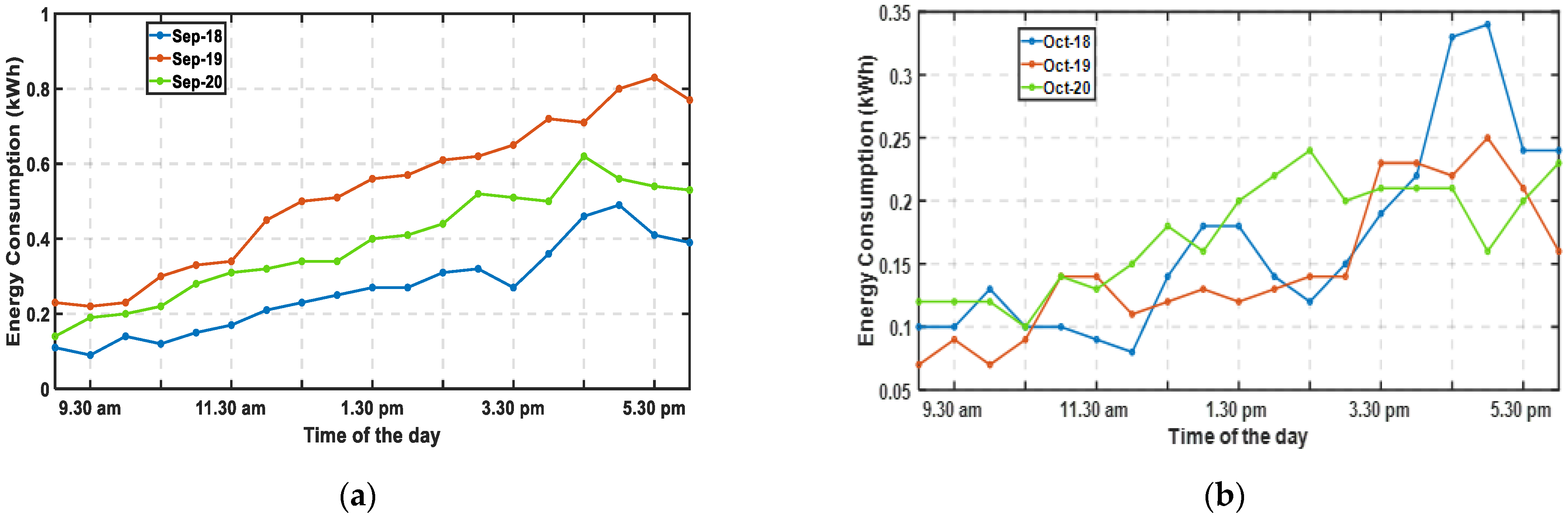
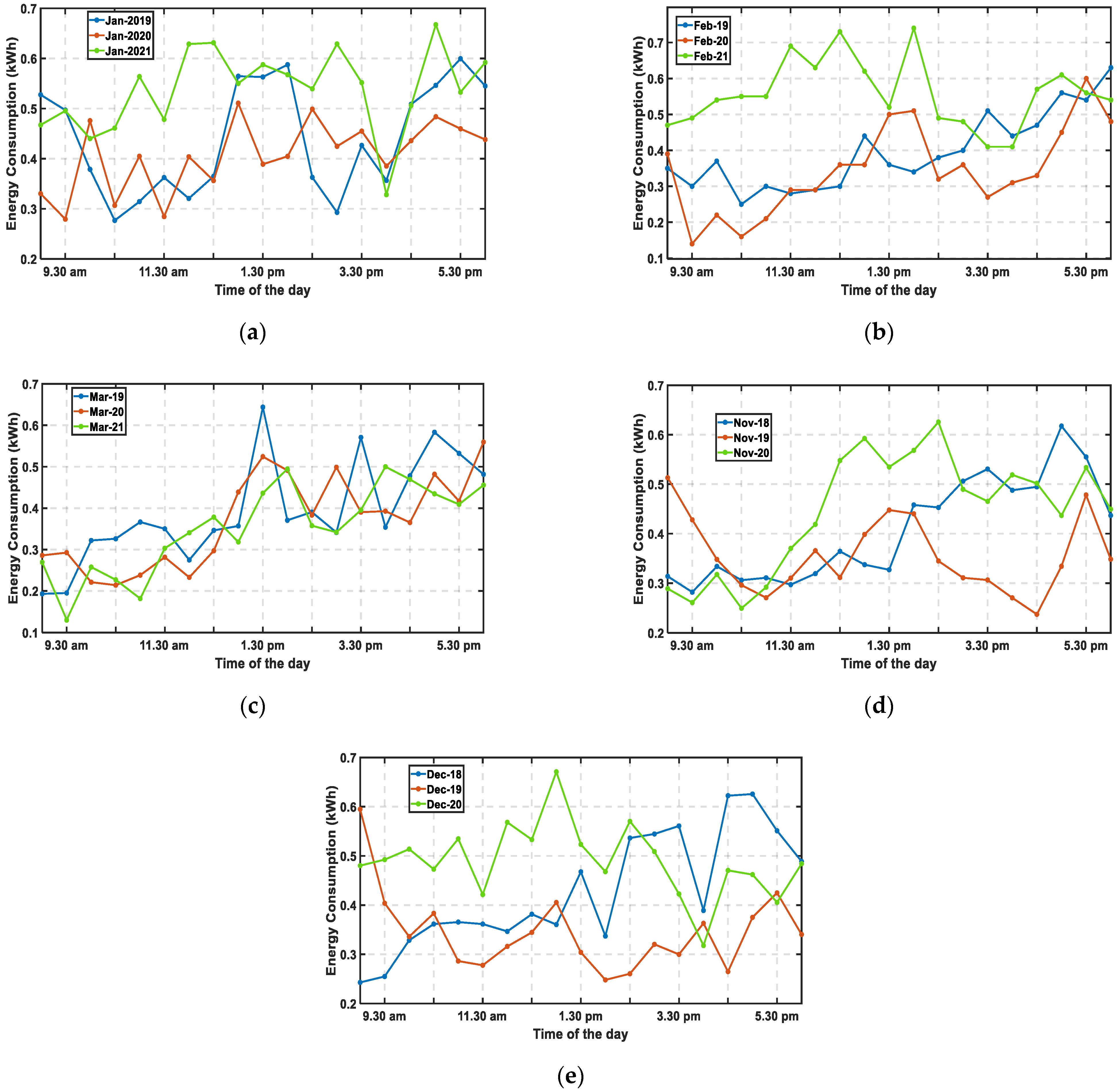
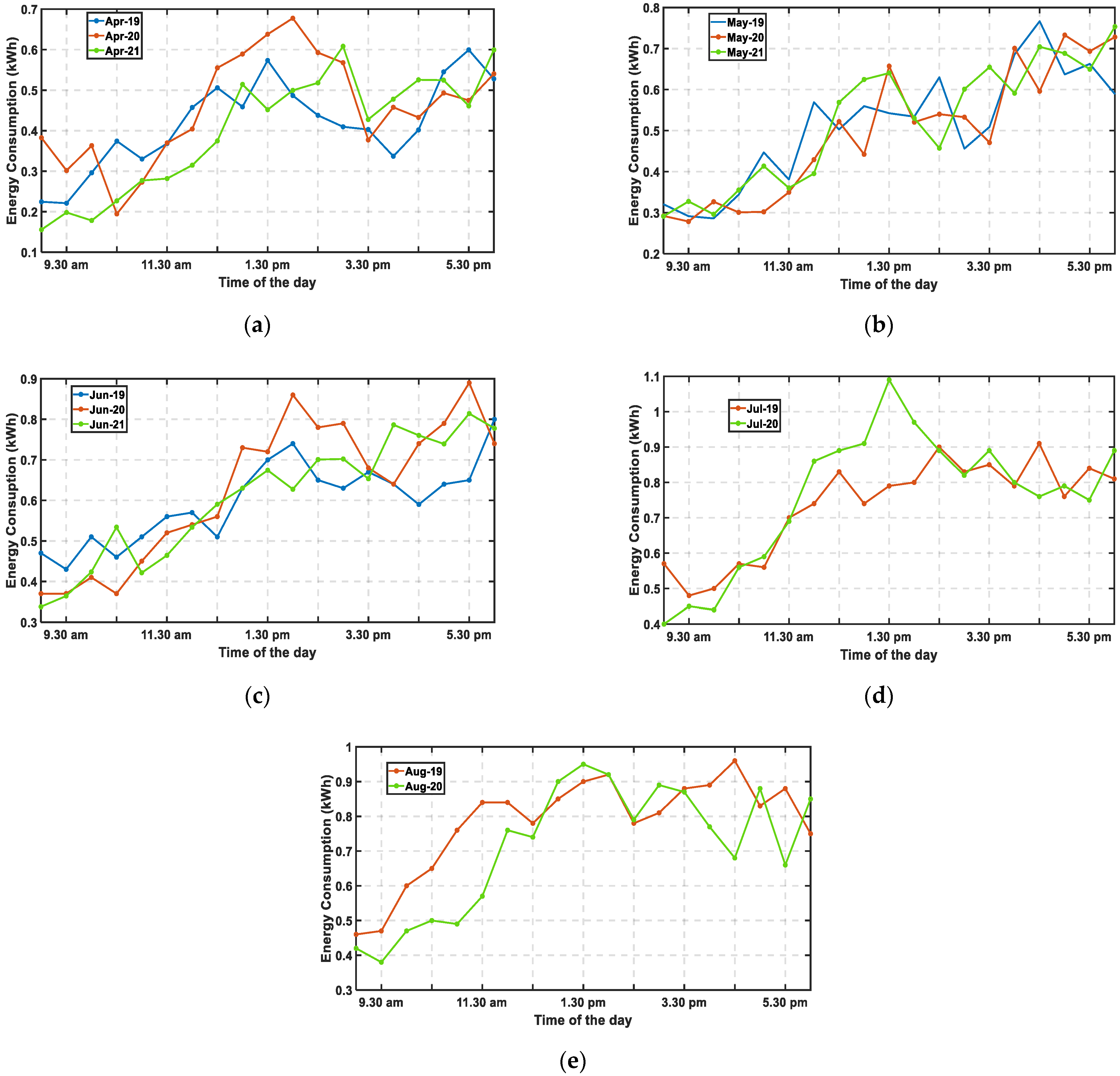
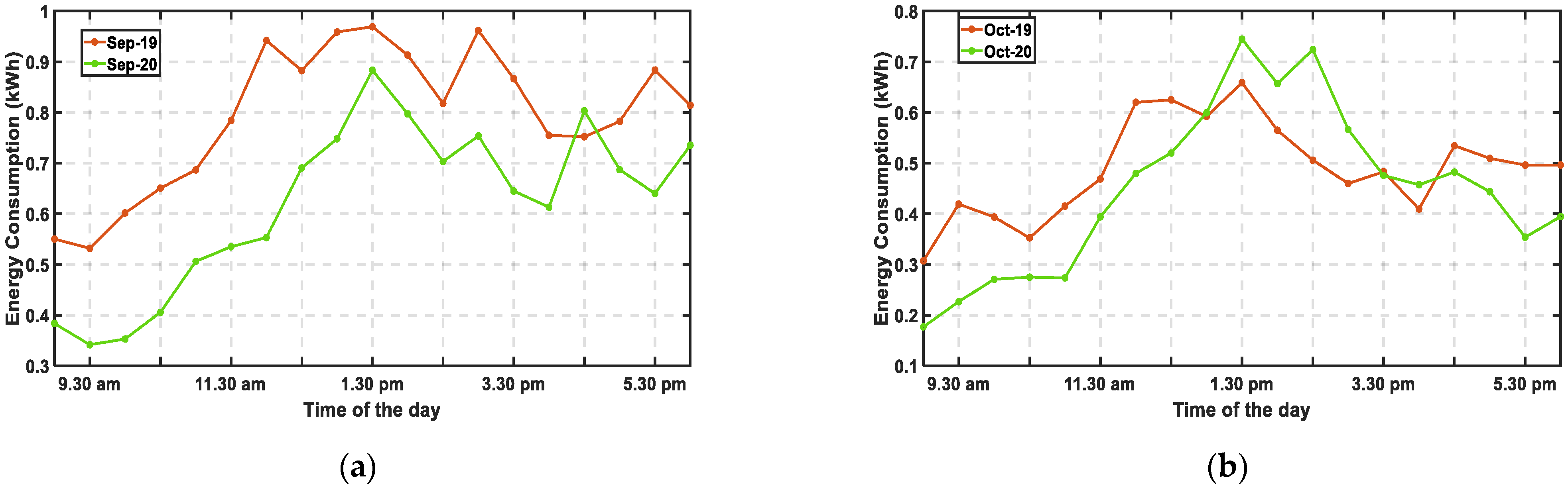
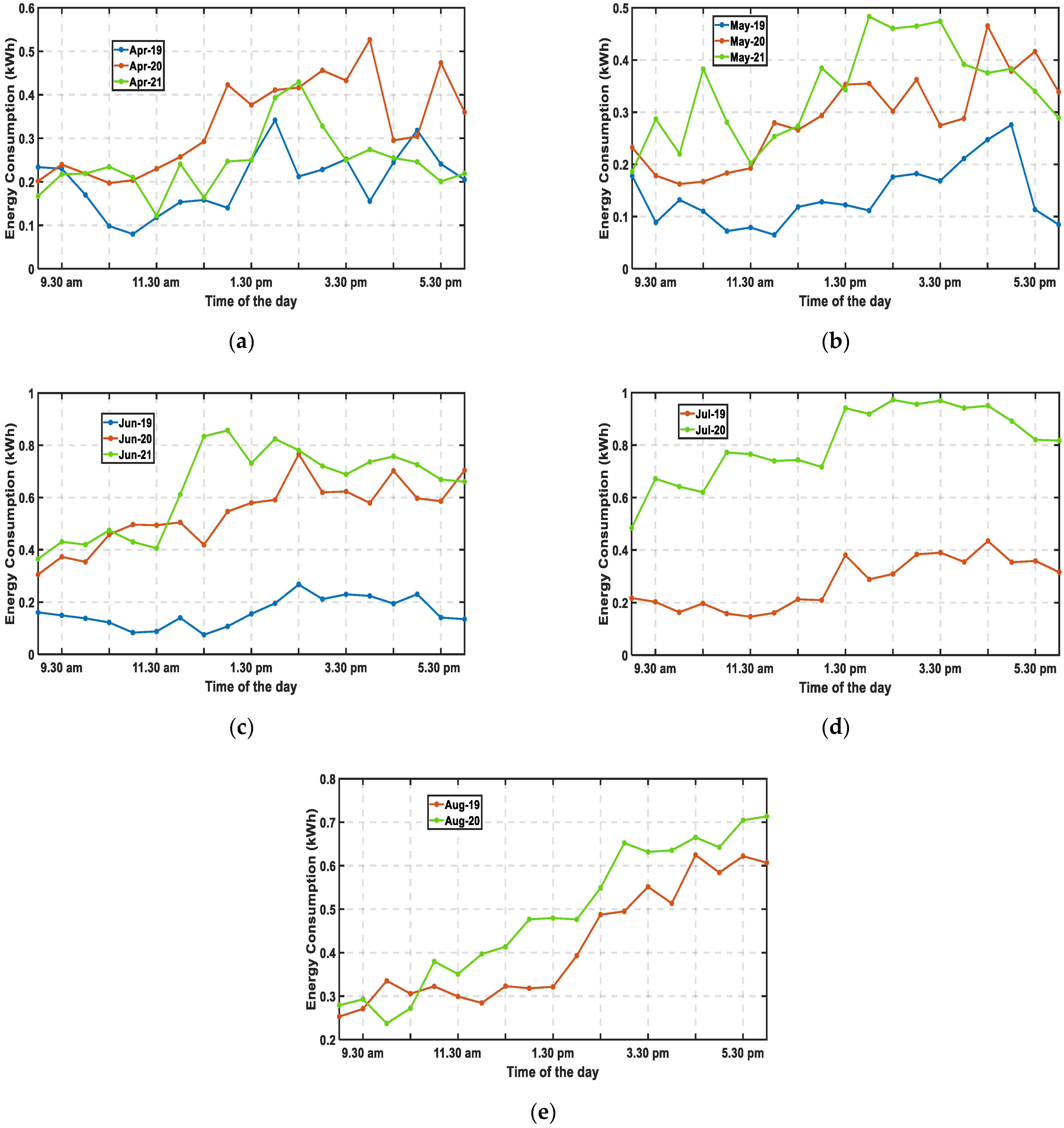
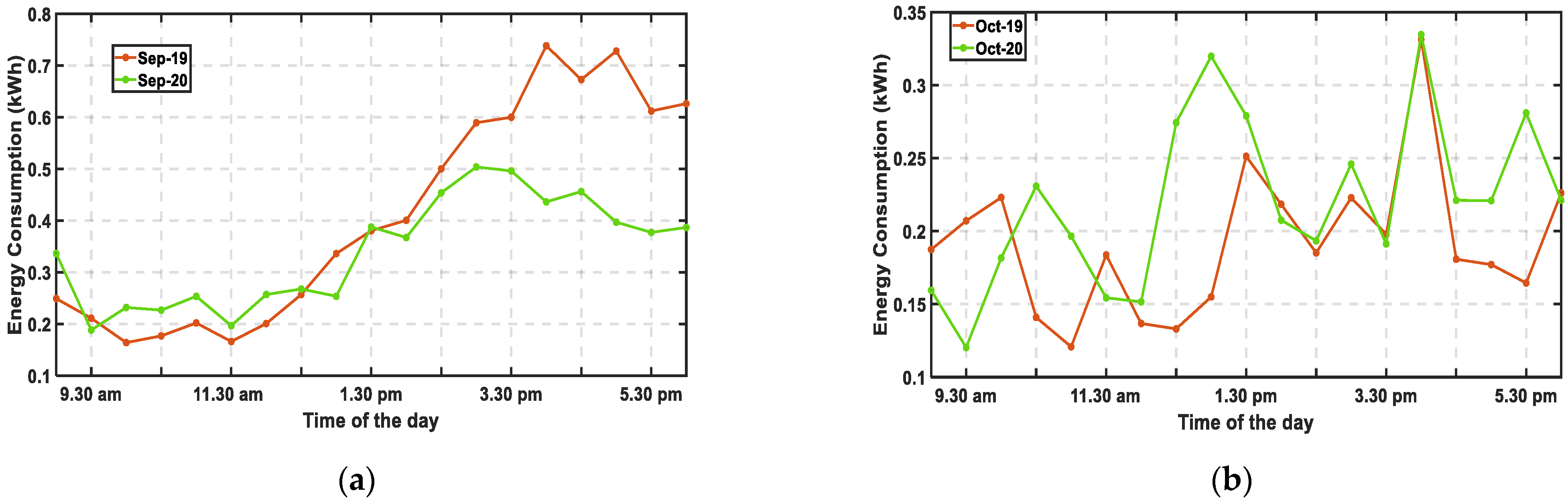
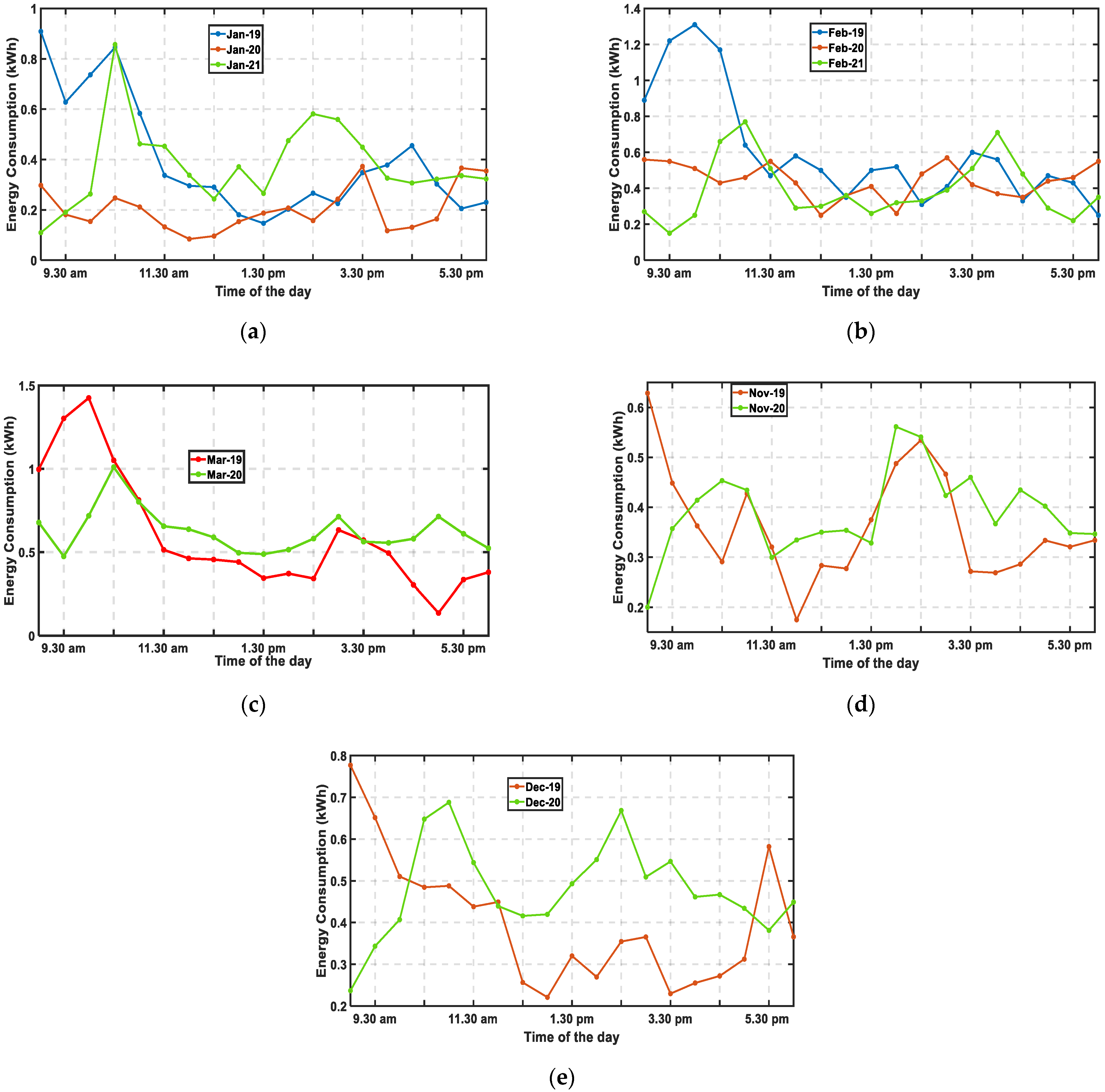
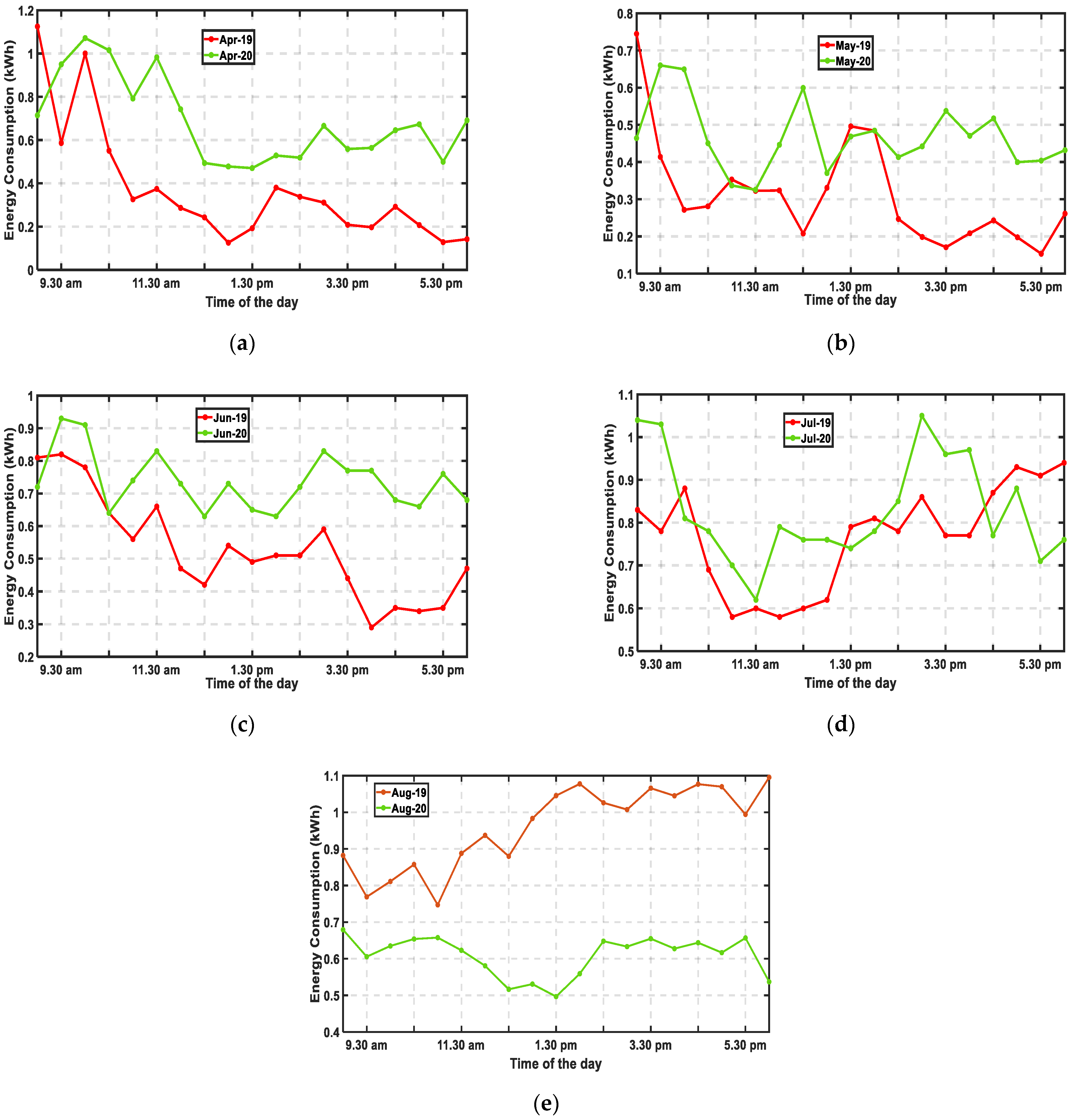
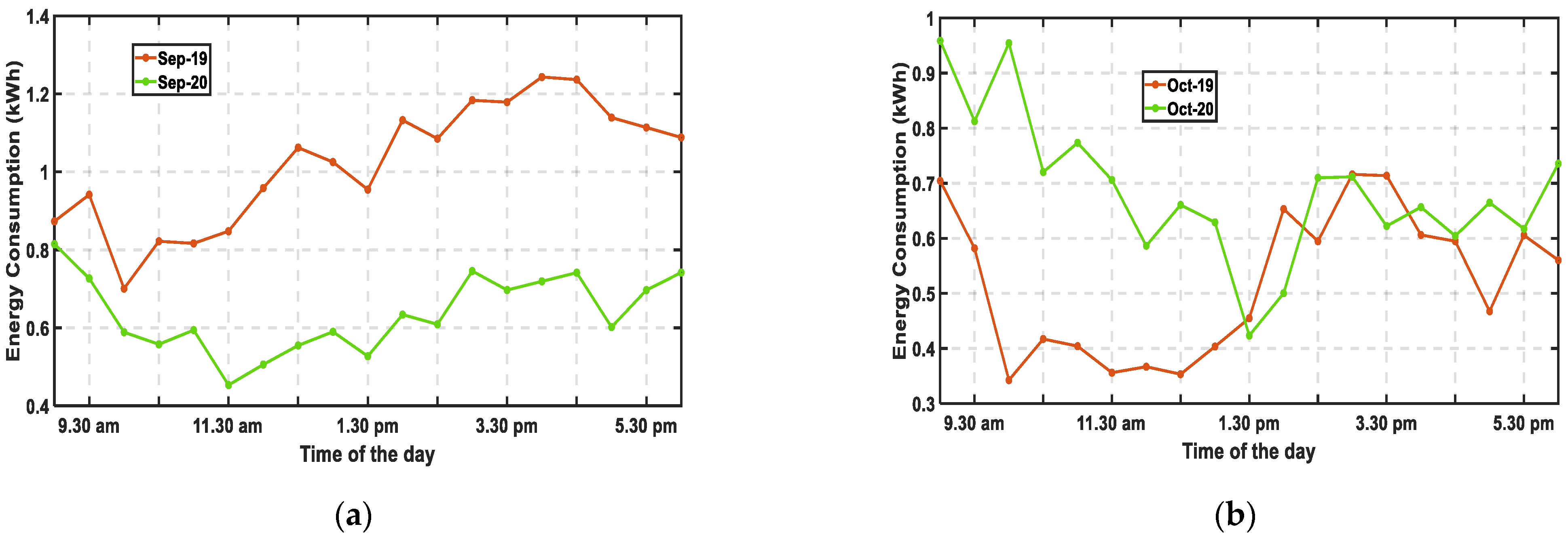
2. Energy Consumption Analysis of Different Consumers

In this section, the energy consumption patterns of four different consumers are analyzed mainly from January 2019 to June 2021. All the energy consumptions before 24 March 2020, is considered as pre-COVID energy consumption as complete lockdown was first enforced from this day. Therefore, the energy consumptions from April 2020 to June 2021 is considered as energy consumption data during COVID situations. All the consumers live in Memphis city, Tennessee, USA. The energy consumption data of all the consumers were collected by smart meter and available in Memphis Light Gas water (MLGW) database.

2.1. Consumer 1

For consumer 1, two of the family members work outside during the office hours but working from home since the lockdown due to COVID 19 pandemic. For consumer 1, data of energy consumption from August 2018 to June 2021, are available. The energy consumption data for the months from November to March are shown in Figure 1, when temperatures normally remain lower (below 65 °F). The average energy consumption, as shown in Figure 1, indicate that the energy consumption of consumer 1 has increased during office hours (from 9:00 a.m. to 6:00 p.m.). For the month of January (Figure 1a), the energy consumption after COVID-19 (January 21) has increased almost all hours than that of pre-COVID time (January 2019 and January 2020). Similar situation is observed for the month of February (Figure 1b). However, for the month of March, the energy consumption after COVID-19 (March 2021) has increased almost from 12:30 p.m. to 6:00 p.m. than that of pre-COVID time (March 2019 and March 2020), specially March 2020. For the month of November, the energy consumption has increased for almost all office hours in November 2020 than that of November 2018 and 2019 (pre-COVID situation). Similar situation is observed for the month of December.

Moreover, the energy consumptions of consumer 1, for the month from April to August when temperatures normally remain high (above 65 °F), are shown in Figure 2. For the month of April in 2020 and 2021 (after COVID-19 situation), the energy consumption is higher than that in April 2019.

Moreover, for the month of May 2021, the energy consumption is much higher than that in May 2020 and May 2019 where the energy consumption in May 2020 is higher that of May 2019, mostly from 9:00 a.m. to 3:30 p.m. The energy consumption pattern in June 2020 is higher than that of June 2019 from 9:30 a.m. to 12:30 p.m., and from 4:00 p.m. to 6:00 p.m.

In addition, from Figure 2d, it is evident that the consumer 1 consumed much more energy in July 2020 as compared to July 2019. However, energy consumed by consumer 1 in August 2020 is higher that of August 2018, but lower than that of August 2019 from 1:30 p.m.

Almost similar situation is observed for the month of September, as shown in Figure 3a. For the month of October, as shown in Figure 3b, the energy consumption in 2020 is higher than that of 2019 and 2018 almost from 9:00 a.m. to 3:00 p.m.

2.2. Consumer 2

As for the consumer 2, two of the four members usually stay outside home during office hours for work and school during normal time, and other two remain at home all the time of the day, but during the COVID period, all of them have been forced to stay at home. The energy consumption of consumer 2 from January to March for the years from 2019 to 2021 is shown in Figure 4a to Figure 4c, respectively.

Similar to Consumer 1, Consumer 2 consumes more average energy for all hours in January 2021 than that in 2019. Similar scenario is also observed for energy consumption in January 2021 and January 2019. Moreover, the consumption in February 2021 (after COVID situation) is higher for almost all hours as compared to that in February 2019 and 2020. However, for the month of March, exactly different situation is observed where the energy consumptions in 2019 and 2020 (pre-COVID conditions) are higher than that in 2021.

Moreover, consumption in November and December for the years from 2019 to 2021 are shown in Figure 4d and Figure 4e, respectively which indicate that the energy consumption for the November and December in 2020 (after COVID situation) is higher than that of in 2018 and 2019 from 11:30 a.m. to 2:30 p.m., and from 9:30 a.m. to 2:30 p.m., respectively.

The energy consumption for the months from April to June for Consumer 2 for the consecutive three years (2019 to 2021) are shown in Figure 5. The consumption is higher for both April 2020 and 2021 almost for all hours from 1:00 p.m. to 4:00 p.m. than that in April 2019.

From Figure 6, it is evident that the energy consumption during the office hours is higher in pre-COVID conditions than that in COVID conditions for the month of September (Figure 6a). However, for the month of October, the energy consumption is higher for almost all hours from 1:00 p.m. to 4:00 p.m. in 2020 as compared to the energy consumption in 2019.

2.3. Consumer 3

As for the Consumer 3, energy consumption data is analyzed from January 2019 to June 2021. Consumer 3 has three members of which one stays outside during office hours in normal time. Similar to Consumer 1 and Consumer 2, the energy consumptions, for the months from January to March for consecutive three years (from 2019 to 2021) and for the months from November to December for consecutive two years (from 2019 to 2020), are analyzed in Figure 7.

Unlike Consumer 1 and 2, the energy consumption in January 2021 is lower than that of 2020 for almost all office hours (Figure 7a). However, it is higher than the consumption in 2019. Similar situation is observed for the energy consumption in February as shown in Figure 7b.

Figure 7c indicates that the energy consumption in March 21 is lower than the consumption in March 20 or 19 for most of the office hours. However, Consumer 3 has consumed more energy in November 2020 as compared to 2019 for almost all hours from 10:30 a.m. to 2:00 p.m. and from 4:00 p.m. to 6:00 p.m. Similarly, the energy consumption is higher in December 2020 as compared to 2019 for all office hours from 9:00 a.m. to 11:00 a.m. and from 4:00 p.m. to 6:00 p.m., except 5:00 p.m.

Moreover, the energy consumptions, for the months from April to June for consecutive three years (2019 to 2021) and for the months from July to August for two years (2019 to 2020), are shown in Figure 8. From Figure 8a, it is evident that energy consumption in April 2020 and 2021 (post-COVID situation) is higher than the consumption in 2019 from 10:00 a.m. to 4:30 p.m. From Figure 8b,c, it is evident that the energy consumptions in May and June in 2020 and 2021 (after COVID) are much higher than the consumption in 2019 for all office hours. The Consumer 3 has consumed much more energy for all office hours in July 2020 as compared to July 2019 as shown in Figure 8d. The consumption in August 2020 is higher than the consumption in 2019 for all office hours except from 10:00 a.m. to 10:30 a.m., as shown in Figure 8e.

Figure 9a indicates that the energy consumption in September 2020 is higher than that in 2019 from 9:00 a.m. to 12:30 p.m. except 9:30 a.m. However, the energy consumption in October 2020 is higher as compared to in 2019 for all office hours from 10:00 a.m. to 5:30 p.m. except 11:30 a.m., 2:00 p.m., and 3:30 p.m., as shown in Figure 9b.

2.4. Consumer 4

The energy consumption data of Consumer 4 are analyzed from January 2019 to February 2021. Consumer 4 are three members that work outside during office hours in normal times.

From Figure 10a, it is evident that Consumer 4 has consumed more energy in January 2021 than in 2019 and 2020 from all office hours from 10:30 a.m. to 3:30 p.m., except 11:00 a.m. and 12:30 p.m. However, different situation is observed for the month of February when consumption is less in 2021 as compared to that in 2020 and 2019 (as shown in Figure 10b).

For the month of November, the consumer has consumed higher in 2020 as compared to 2019 for all hours from 10:00 a.m. to 6:00 p.m. except 11:30 a.m., 1:30 p.m., and 3:00 p.m., as shown in Figure 10d. Similar situation is observed for the month of December from 10:30 a.m. to 6:00 p.m., except 12:00 p.m. and 5:30 p.m. (Figure 10e).

Moreover, Figure 11 indicates that the energy consumption is much higher in 2021 as compared to that in 2020 for almost all hours for the months from April to June (Figure 11a–c). For the month of July, the energy consumption is higher in 2021 from almost all hours from 9:30 a.m. to 4:30 p.m.

Moreover, the energy consumption for August and September is lower is 2021 than that in 2020 for all office hours as shown in Figure 11e and Figure 12a, respectively. However, from 9:30 a.m. to 1:00 p.m., 2:30 p.m., and from 4:00 p.m. to 6:00 p.m., the energy consumption is higher for the month of October 2020 than in 2019, as shown in Figure 12b.

2.5. Comparative Analysis

The comparative analysis of energy consumption among four consumers are summarized in

Table 1. Comparative analysis of energy consumption for four different consumers.

Time	Months
	Jan	Feb	Mar	Apr	May	Jun	Jul	Aug	Sep	Oct	Nov	Dec
9:00 a.m.	0.25	0.50	0.00	0.25	0.50	0.50	0.50	0.50	0.25	0.50	0.00	0.50
9:30 a.m.	0.75	0.50	0.00	0.50	0.75	0.75	0.50	0.25	0.00	0.50	0.00	0.75
10:00 a.m.	0.25	0.50	0.00	0.75	1.00	0.75	0.50	0.00	0.25	0.25	0.50	0.75
10:30 a.m.	0.75	0.50	0.00	0.75	1.00	0.75	0.50	0.00	0.25	0.50	0.75	0.75
11:00 a.m.	0.50	0.75	0.00	0.75	0.75	0.5	0.75	0.50	0.25	0.75	0.75	0.75
11:30 a.m.	0.75	0.50	0.00	0.75	0.50	0.75	0.50	0.50	0.25	0.25	0.75	0.75
12:00 p.m.	0.75	0.50	0.25	0.75	0.75	0.75	0.75	0.25	0.25	0.75	0.75	0.50
12:30 p.m.	0.75	0.50	0.50	0.75	0.75	1.00	0.75	0.25	0.25	0.75	1.00	0.75
1:00 p.m.	0.50	0.75	0.00	1.00	0.75	0.75	0.75	0.75	0.00	0.75	1.00	0.75
1:30 p.m.	0.75	0.50	0.25	0.75	1.00	0.50	0.75	0.50	0.25	0.50	0.75	0.75
2:00 p.m.	0.50	0.75	0.75	1.00	0.75	0.75	0.75	0.25	0.00	0.50	0.75	0.75
2:30 p.m.	0.75	0.75	0.50	1.00	0.75	0.75	0.50	0.25	0.00	1.00	0.75	0.75
3:00 p.m.	0.75	0.50	0.25	1.00	1.00	0.50	0.50	0.75	0.00	0.75	0.25	0.50
3:30 p.m.	0.50	0.00	0.25	0.75	0.75	0.50	0.75	0.25	0.00	0.00	0.50	0.25
4:00 p.m.	0.00	0.25	0.50	1.00	0.50	1.00	0.50	0.25	0.25	0.75	1.00	0.25
4:30 p.m.	0.75	1.00	0.25	1.00	0.50	1.00	0.50	0.25	0.00	0.50	0.75	0.75
5:00 p.m.	0.50	0.75	0.25	0.50	0.75	1.00	0.50	0.50	0.00	0.50	0.25	0.50
5:30 p.m.	0.25	0.50	0.25	0.50	0.50	1.00	0.50	0.25	0.00	0.50	0.50	0.50
6:00 p.m.	0.50	0.25	0.25	0.75	0.75	0.75	0.75	0.50	0.00	0.25	0.75	0.75

. In the month of June, the values in Table 1 from 9:30 a.m. to 10:30 a.m., is 0.75 which means that energy consumption after COVID situation has increased for three of the four consumers than that in pre-COVID condition. In the same month, from 4:00 p.m. to 5:30 p.m. the value is 1.0, which means that the energy consumption has increased for all the consumers (four out of four consumers). However, from 9:00 a.m. to 11:30 a.m. in March, the values are 0, which mean energy consumption has not increased for any consumer.

Based on Table 1, the energy consumptions have been increased significantly from April to July, and then from November to December, as the average increase is above 60% during office hours. Similarly, the average increase is above 50% but is less than 60% for the months of January, February, and October months. For rest of the months increase is less than 40% with increase in consumption in September has least percentage (12%). Based on this analysis, it is observed that the impact on the distribution transformer is higher during COVID-19 period from April to July during office hours as the ambient temperature remains higher during these months. In addition, the loading of the transformer has increased more than or equal to 50% for almost all office hours. Moreover, for the months of November and December, the ambient temperature remains lower. Therefore, some of the increased loading impact can be minimized by the outer lower ambient temperature. The values in Table 1 are used as P (multiplication factor) to determine transformer loading (Per unit current) during office hours as shown in (1).

3. Impacts of Energy Consumption on Distribution Transformer

As the per unit current increases in distribution transformer, its hottest spot temperature (HST), top-oil temperature (TOT), and the percentage loss of life (%LOL) are also increased. Moreover, with the increase in harmonics in currents produced by non-linear load that are used in the household, HST, TOT, and %LOL increase. Therefore, per unit current in distribution transformer and the harmonics contents in currents are necessary to analyze the detrimental impact of increased loads in terms of HWT, TOT, and % LOL.

3.1. Determination of Per Unit Current of Distribution Transformer

The per unit current in distribution transformer can be calculated using the following equation:

$$T_{pu}=\frac{I_i\times n\times P}{I_{Trated}}$$

(1)

where T_pu and I_Trated are the per unit and rated current of the distribution transformer, respectively. I_i, n are the current of individual consumer and number of consumers under the considered transformer, respectively. P is the factor that determines what would be the multiplication factor with the individual current of consumer (I_i) to determine the per unit current as different consumer has different consumption patterns. If the value of p is 0.75, it indicates that total current of distribution transformer will be 0.75n times of individual consumer current (I_i) rather than n times.

The per unit currents of distribution transformer for the months of April and June during office hours using (1), are shown

Table 2. Per unit current of transformer for different months.

Time	April			June
	2019	2020	2021	2019	2020	2021
9:00 a.m.	0.02	0.03	0.05	0.04	0.17	0.26
9:30 a.m.	0.04	0.06	0.14	0.17	0.26	0.46
10:00 a.m.	0.05	0.11	0.17	0.19	0.29	0.56
10:30 a.m.	0.04	0.10	0.24	0.23	0.43	0.62
11:00 a.m.	0.05	0.11	0.30	0.19	0.24	0.33
11:30 a.m.	0.04	0.12	0.31	0.35	0.44	0.55
12:00 p.m.	0.04	0.07	0.36	0.32	0.41	0.69
12:30 p.m.	0.05	0.08	0.43	0.40	0.46	0.99
1:00 p.m.	0.12	0.14	0.88	0.44	0.35	0.82
1:30 p.m.	0.09	0.12	0.47	0.36	0.29	0.53
2:00 p.m.	0.07	0.26	0.78	0.49	0.46	0.83
2:30 p.m.	0.13	0.35	0.80	0.52	0.47	0.86
3:00 p.m.	0.04	0.38	0.94	0.45	0.42	0.62
3:30 p.m.	0.05	0.21	0.42	0.46	0.44	0.52
4:00 p.m.	0.12	0.20	0.64	0.88	0.93	1.25
4:30 p.m.	0.18	0.26	0.77	0.74	0.90	1.27
5:00 p.m.	0.08	0.11	0.36	0.80	0.96	1.24
5:30 p.m.	0.06	0.11	0.30	0.69	1.01	1.37
6:00 p.m.	0.14	0.25	0.67	0.54	0.74	1.38

. The currents of Consumer 1 is considered as individual consumer current (I_i). The value of n is 6 and p are taken from Table 1, which is more realistic approach as it is determined from the energy consumption data available from both pre-COVID and during COVID conditions for four consumers as Table 1 shows the probability of loads to increase during office hours. From Table 2, it is evident that the per unit current of transformer for 2020 to 2021 has increased as compared to that in 2019.

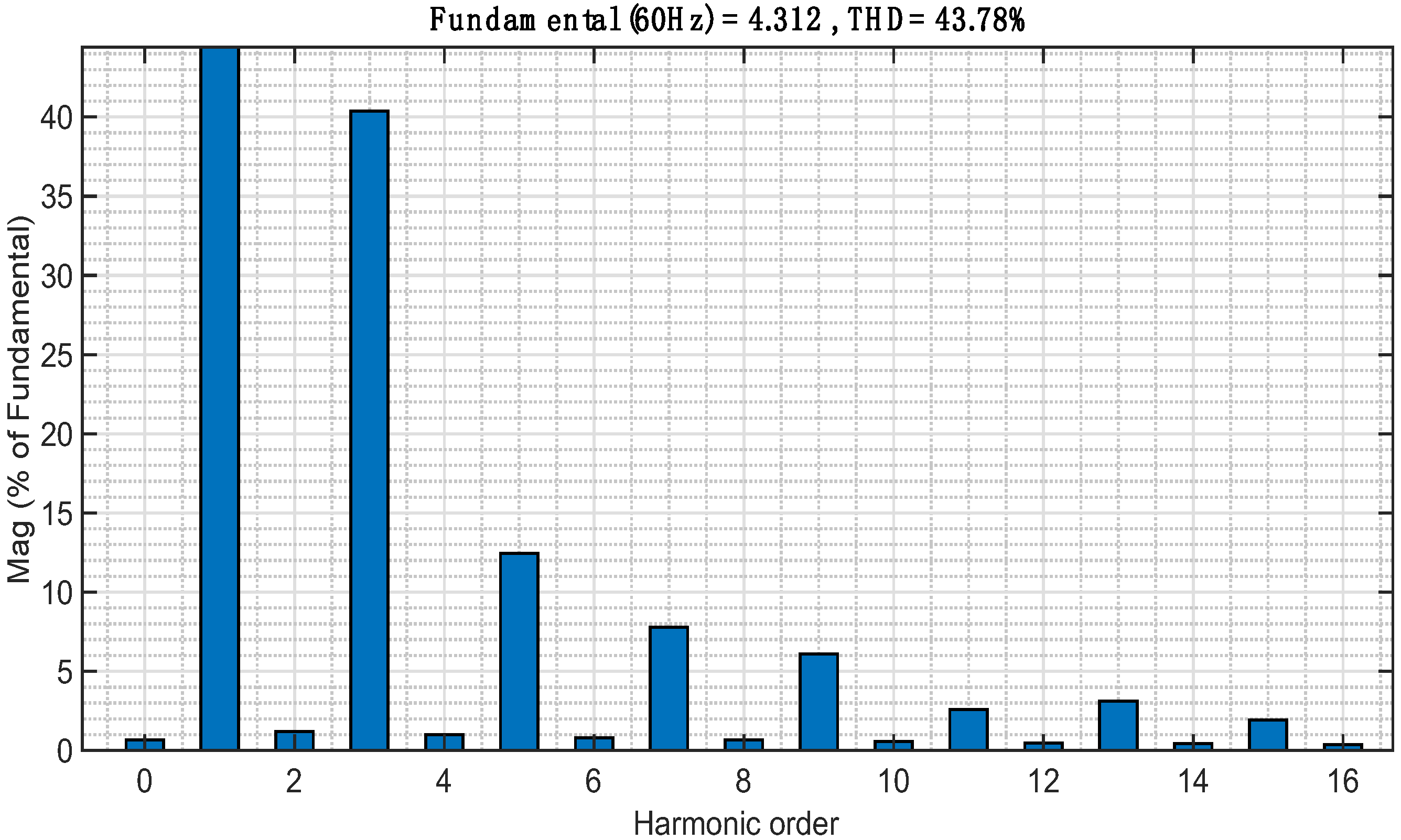
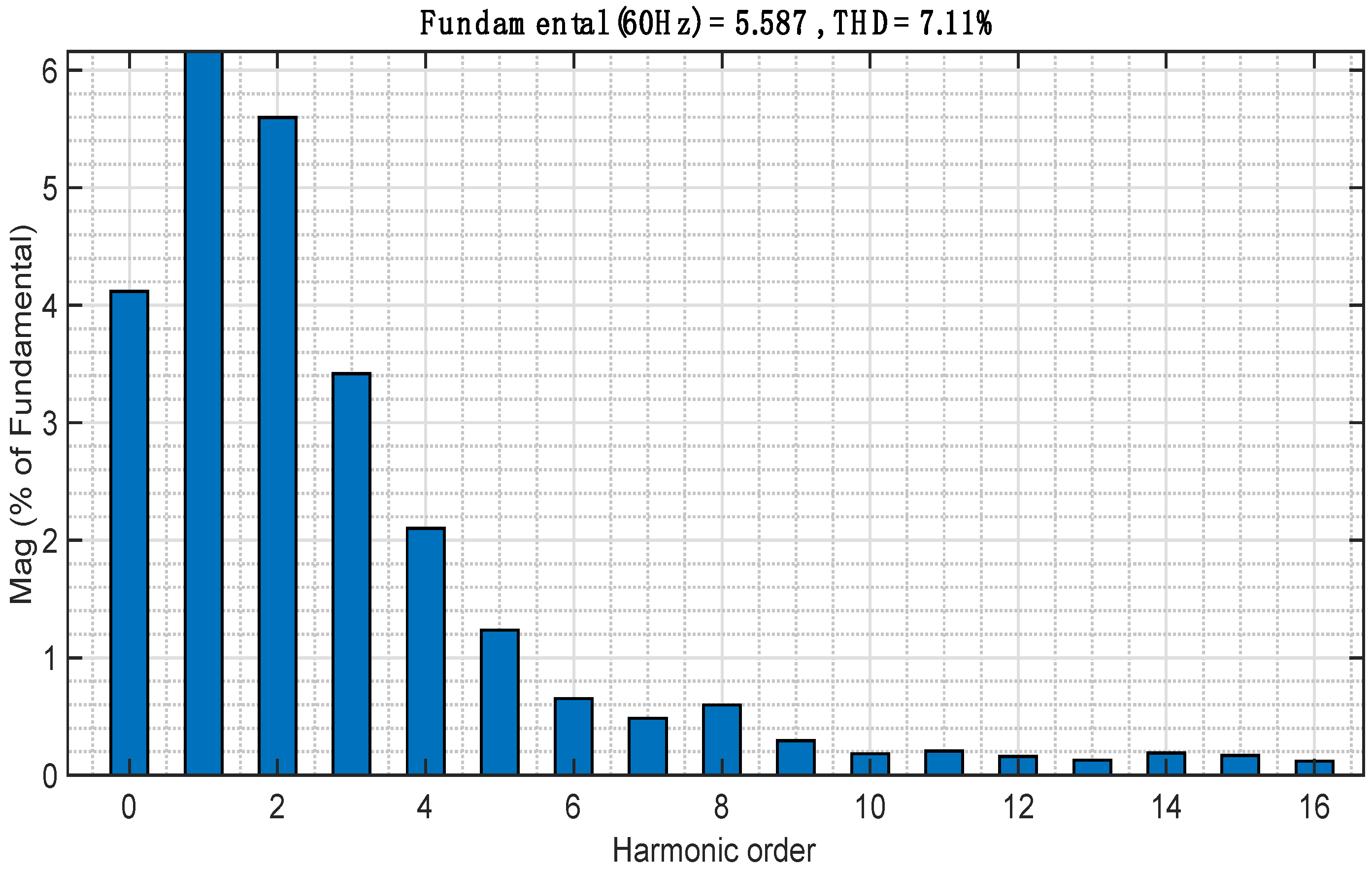
3.2. Determination of Harmonic Content in Current of Distribution Transformer

As discussed, the harmonics in currents produce rise in temperature and %LOL. Therefore, harmonics in currents is required to calculate harmonic loss factor (F_HL) and harmonic loss factor for other stray loss (F_HL-STR), as shown in (2) and (3), respectively [21].

$$F_{HL}=\frac{{\sum }_{h=1}^{\infty }{\left(\frac{I_h}{I_1}\right)}^2{h}^2}{{\sum }_{h=1}^{\infty }{\left(\frac{I_h}{I_1}\right)}^2}=\frac{{\sum }_{h=1}^{\infty }{\left(\frac{I_h}{I_L}\right)}^2{h}^2}{{\sum }_{h=1}^{\infty }{\left(\frac{I_h}{I_L}\right)}^2}$$

(2)

$$F_{HL-STR}=\frac{{\sum }_{h=1}^{\infty }{\left(\frac{I_h}{I_1}\right)}^2{h}^{0.8}}{{\sum }_{h=1}^{\infty }{\left(\frac{I_h}{I_1}\right)}^2}=\frac{{\sum }_{h=1}^{\infty }{\left(\frac{I_h}{I_L}\right)}^2{h}^{0.8}}{{\sum }_{h=1}^{\infty }{\left(\frac{I_h}{I_L}\right)}^2}$$

(3)

In order to analyze the harmonic contents in current, an experimental lab setup with transformer and non-linear load are considered, as shown in Figure 13. The system shown in Figure 13 consists of an AC 208 V, 60 Hz power supply a 1 kVA distribution transformer, supplying a nonlinear DC load of 150 W and RL AC loads. The nonlinear load is a controlled rectifier that produces odd harmonics, most prominently the third harmonic, as shown in Figure 14, and has total harmonic distortion (THD) of 43.78%. Based on the harmonic content, using (2) and (3), the values of F_HL and F_{HL_STR} are calculated as 3.19 and 1.27, respectively.

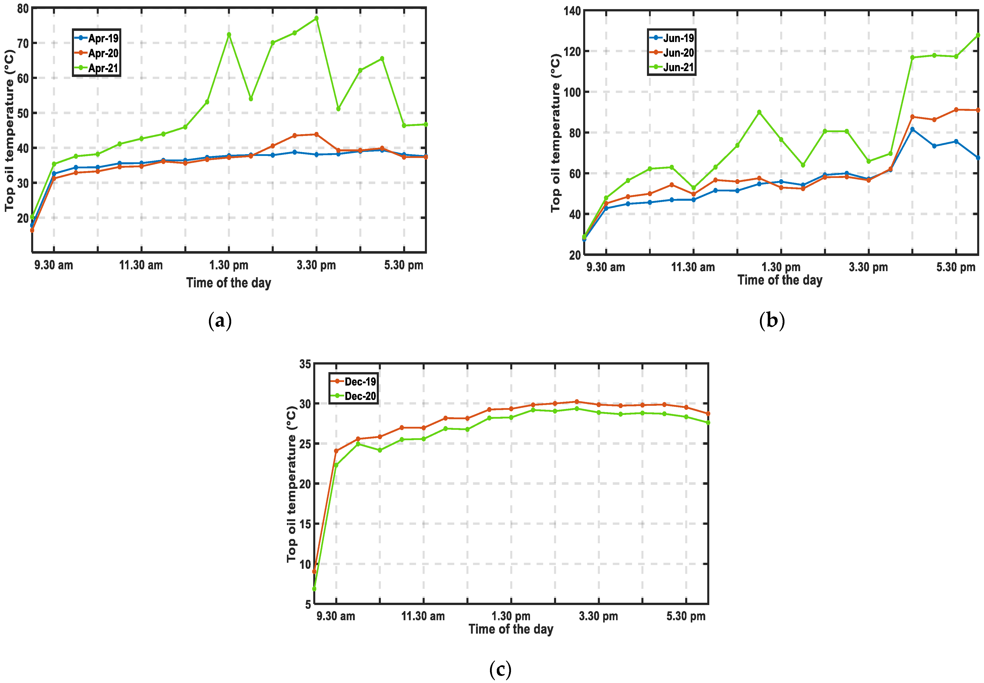
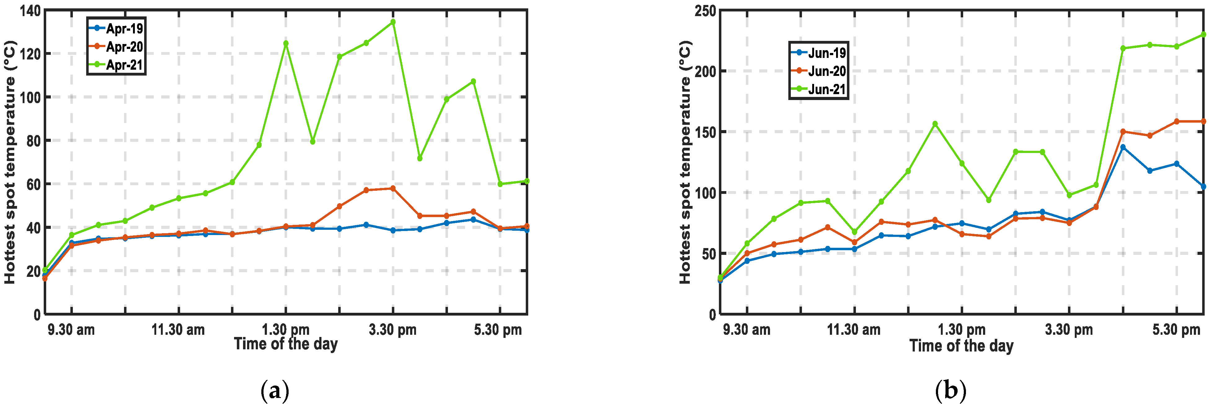
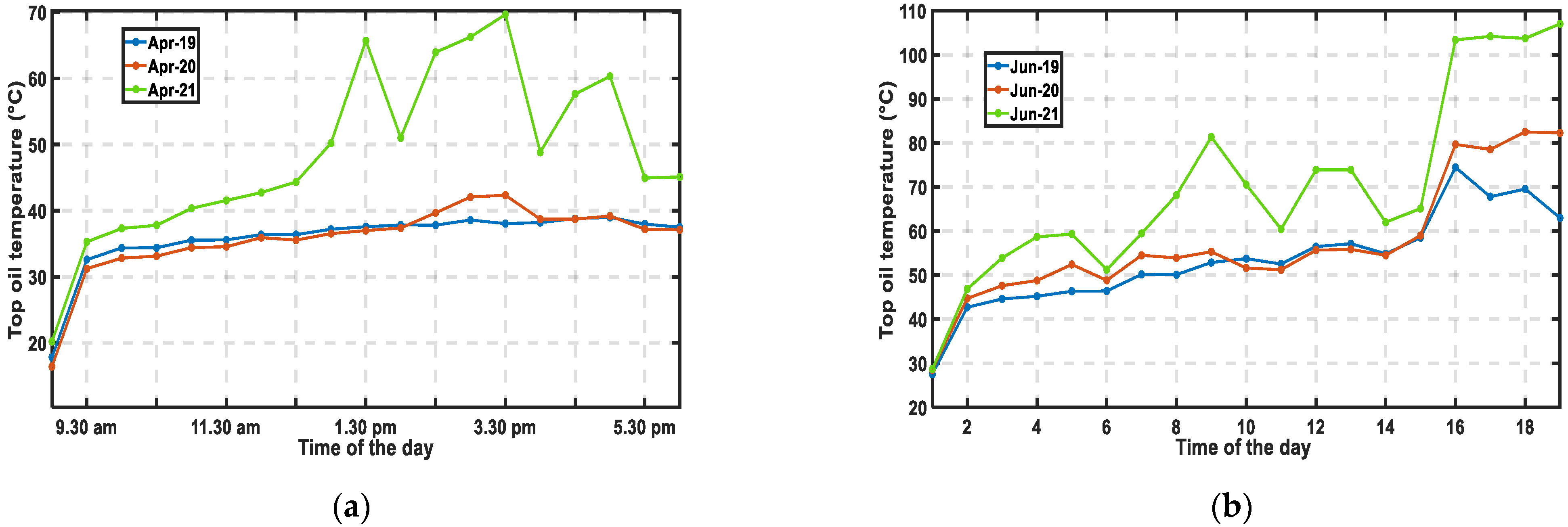
3.3. Calculation of Hottest Spot, Top Oil Temperature of Distribution Transformer

Based on the per unit transformer current and calculated values of F_HL and F_{HL_STR}, the hottest winding temperatures of transformer for the month of April, June, and December are shown in Figure 15 as the average energy consumption has increased 76%, 75%, and 63%, respectively, for these months.

The operating conditions, such as hottest spot temperature, top-oil temperature, and loss of life, are calculated by the equations as in [21] and simulated in MATLAB.

IEEE standard C57.91-2011 recommends that the hottest spot temperature of transformer winding should be kept below 200 °C to prevent failure of transformer. It is evident from Figure 15a that the temperature remains close to 150 °C from 1:30 p.m. to 3:00 p.m., and goes beyond 150 °C for April 2021.

For April in 2020 and 2019, the hottest spot temperature remains well below 80 °C. Moreover, for June 2021, the temperature remains above 200 °C from 4:30 p.m. to 6:00 p.m. For June 2020 and June 2019, respectively, the temperatures always remain under 200 °C. However, although the energy consumption has been increased in December 2020, the hottest spot temperature in both 2020 and 2019 is below 50 °C for all office hours as the ambient temperature is remained much lower as compared to that in April and June.

Moreover, the top oil temperatures for the months of April, June, and December are shown in Figure 16. Figure 16a,b indicate that the temperature never goes beyond 120 °C, as recommended by IEEE standard C57.91-2011 to prevent transformer failure, for April and December, respectively. Similar situations are observed for April 2020 and 2019 (Figure 16a). However, temperature goes beyond 120 °C for June 2021 at 6:00 p.m., as shown in Figure 16c.

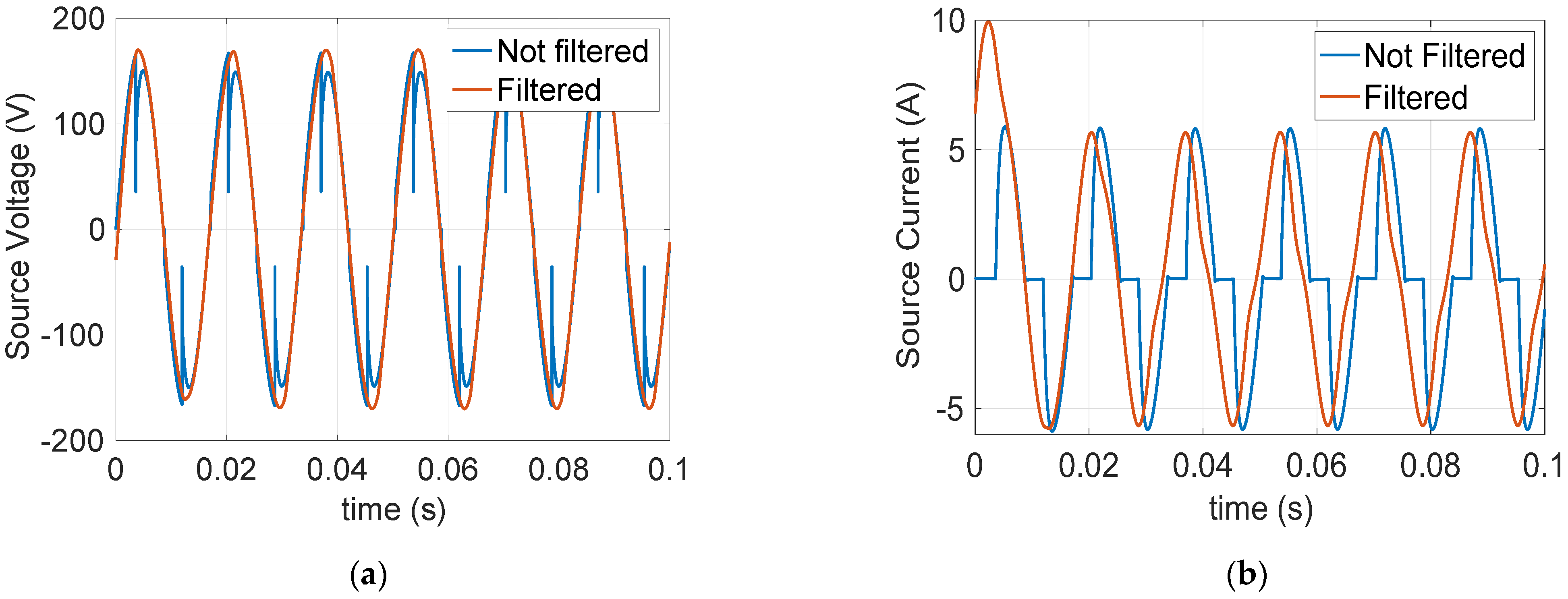
4. Proposed Mitigation Technique

As the harmonics in currents plays pivotal role in increasing hottest spot temperature, top-oil temperature, and loss of life; therefore, in this work, a harmonic filter at the residential side is proposed to reduce the harmonics in currents provided by the transformer.

4.1. Filter Design

The transfer function of the LC filter can be calculated as:

$$TF\left(s\right)=\frac{1}{1+\frac{R_d{C}_f}{n+1}·s+s^2·L_f·C_f·\frac{n}{n+1}}$$

(4)

where, C_f and L_f the filters capacitor and inductor, respectively. R_d and L_d are the damping resistor and inductor. n is the damping ratio and can be expressed as:

$$n=\frac{L_d}{L_f}$$

(5)

The damping factor can be calculated as:

$$\zeta =\frac{1}{2}·\frac{R_d}{n+1}·\frac{\sqrt{C_f}}{\sqrt{L_f}}$$

(6)

and the damping resistance is:

$$R_d=2·\zeta ·\left(n+1\right)· \frac{\sqrt{L_f}}{\sqrt{C_f}}$$

(7)

The transformer voltage and current with and without filter are shown in Figure 17a,b, respectively.

It is essential as the loads that are used during office hours, such as laptop, computer, mobile charger, etc., are non-linear DC loads and produce higher components of harmonics in currents. Figure 18 shows the experimental setup of ac 208 V, 60 Hz power supply by a 1 kVA distribution transformer, supplying a nonlinear load of 150 W via an LC filter with a series RL damping branch. After experimenting with different combination of AC and DC load with and without the LC filter, the results are summarized in

Table 3. THD for different combination AC and DC loads with/without LC filter.

	Case 1	Case 2	Case 3	Case 4	Case 5	Case 6	Case 7	Case 8
	With RLC	With RLC	With RLC	With RLC	W/O RLC	W/O RLC	W/O RLC	W/O RLC
Readings	With RL	Without RL	With RL	Without RL	With RL	Without RL	With RL	Without RL
V(AC) (RMS)	120.6	120.5	121.39	121.6	119.5	119.97	120.32	121.4
I(AC) (RMS)	3.4	3.28	2.82	2.8	4.76	4.2	2.56	2.16
V(DC)	63.3	66.4	40	40	95.2	94.1	40	40
I(DC)	2.45	2.58	1.55	1.55	3.68	3.64	1.55	1.55
THD%	6.50	6.60	16.80	20	9.60	11.00	45.50	56.20

, which indicates the impact of RL AC load has minimal impact on THD whereas DC loads are responsible for producing harmonics and THD. The values of L_f and C_f of LC filter are selected to be 70 mH and 100 µF, respectively. Considering n = 2/15, the values of the R_d and L_d of RL damping branch are calculated to be 26.39 Ω and 9.3 mH, respectively. Due to the inclusion of harmonic filter, the hormonic content in transformer current is reduced resulting in reduction in total harmonic distortion to 7.11% (as shown in Figure 19) as compared to that of 43.78% (as shown in Figure 14).

The power loss of the system with and without filters are demonstrated in Figure 20 which clearly indicate the efficacy of the proposed solution in reducing transformer loss, and thus the proposed system reduces temperature rise in distribution transformer without forcing the consumer to sacrifice or schedule their load demands during office hours.

4.2. Efficacy of the Proposed Mitigation Technique in Hottest Spot, Top Oil Temperature and Percentage of Loss Reduction in Distribution Transformer

As the harmonics component in the current provided by the distribution transformer is reduced by harmonic filter at the residential side, the hottest spot temperature of the transformer winding, top oil temperature, and percentage loss of life transformer are reduced significantly. Figure 21a suggests that the hottest spot temperature is far below 200 °C (140 °C) for April 2021, which is recommended, with the system having harmonic filter at the residential side. From Figure 21b, it is evident that the temperatures never exceed above 200 °C for June 2019 with harmonic filter. For the month of June 2021, the increase in consumption resulted in increase in temperature above 200 °C from 12:30 p.m. to 6:00 p.m. without filter (Figure 15b), but the temperature is still reduced almost 30 °C with filter in the system, as shown in Figure 21b.

Similarly, the top oil temperature for the month of April in 2021, 2020, and 2019 a with filter is reduced (Figure 22a) as compared to the system without filter (Figure 16a). From Figure 16b, it is evident that the top oil temperature without filter remain close to 120 °C from 4:30 p.m. to 5:30 p.m., and temperature remains slightly above 120 °C at 6:00 p.m. However, for the system with filter, the top oil temperatures always remain under 110 °C. Therefore, the temperature is reduced with the inclusion of harmonic filter at the residential side.

The percentage loss of life (%LOL) of transformer for the months of April, June, and December is summarized in

Table 4. Percentage loss of transformer life (%LOL).

Month	Year	Without Filter (%)	With Filter (%)	Reduction in Loss of Life (%)
April	2019	2.10 × 10−7	1.94 × 10−7	7.55
	2020	9.78 × 10−7	5.96 × 10−7	39.04
	2021	1.11 × 10−2	1.87 × 10−3	83.12
June	2019	0.009	0.002	81.75
	2020	0.131	0.020	85.06
	2021	36.728	2.515	93.15
December	2019	5.19 × 10−8	4.86 × 10−8	6.37
	2020	5.02 × 10−8	4.53 × 10−8	9.80

. From Table 4, it is evident that the loss of life is reduced significantly for the system with filter than that of system without filter. Moreover, the loss of life in June is higher as compared to that in April and December. In June 2021, the loss of life is 36.726% which, when the filter is used, the loss goes down to 2.515%, although energy consumption is increased significantly in 2021 as compared to previous years.

4.3. Energy Saving Recommendations

This section provides a guideline for utilities to alleviate transformers overloading and avoid potential power outages during in any future emergencies where work from home is mandated. The energy saving solutions, which are gathered and proposed in this paper, can be categorized into two groups: (1) low-cost solutions, and (2) transformative solutions.

Low-cost solutions are resilient, simpler, and quicker to implement in emergencies. These methods include (i) reducing the loads capacity or creating capacity [22]. Capacity can be created by getting rid of legacy equipment old, inefficient devices. Turning off unnecessary devices (Plug Load Management [23]), and upgrading to more energy efficient and battery powered equipment. (ii) Improving residential HVAC system to allow for better ventilation, better airflow, and smart temperature regulation, shutoff AC for areas that are not in use during peak hours. Maybe moving the central AC controller and sensor to an optimized location in the house. Residential HVAC efficiency can also be increased, in the long term, by window glazing, house insulation, and caulking glass windows and doors. (iii) Smart HVAC controllers and house energy management systems as described in [24] can reduce energy consumption. (iv) Off-peak load rescheduling is proposed in [21]. (v) In addition to rescheduling loads, rescheduling working hours is also possible through incentives for non-essential workers working from home. (vi) IoT Enabled metering can make consumers more conscious of their energy consumption habits and emissions [25]. (vii) Transformers cooling through better ventilation, passive cooling, reflective tank paint, and shading [26]. Although they are costly and complex, transformative solutions have benefits which may include greater resiliency, improved power quality and reliability, and the longer life cycle of equipment and loads. These methods include (i) upgrading to energy efficient transformers, such as amorphous core transformers (AMTs), that provide superior efficiency and lower iron losses than regular transformers [27]. (ii) Small power factor correction capacitors at the terminal of the transformer to reduce the reactive power losses in the transformer due to compressors’ reactive currents I_x²R [28]. (iii) Active and passive filters. (iv) Behind the meter generation, battery energy storage as proposed in [21]. (v) Telecom utilities, in the US, are required by law, to have battery energy storage on board in the case of power outage.

Telecom towers can be utilized for power systems demand-response applications [29]. (vi) Combined Cooling, Heat & Power (CCHP) for residential and commercial buildings [30] may reduce the energy consumption. (vii) Given that most of the consumer end loads are DC, i.e., laptops, TV, lights, or can be transformed to DC, i.e., washing machines and refrigerators, converting the residential systems to a fully Low voltage DC network may increase the system efficiency. The DC system reported in [31] is 6% more efficient than the equivalent AC system during the day and 17% more efficient during the night. (vii) Solid State Transformers (SST) can be used to reroute energy from one transformer to another as needed when the low voltage secondary circuits are interconnected [32].

To assist in prioritizing energy solutions across a range of scenarios, Figure 23 depicts a value and cost for each solution. Value and cost metrics were determined based on qualitative measures and the documents cited in this paper. The x-axis is showing the expected value of the presented method assigned based on the relative potential for energy and energy cost savings with solution implementation, where “1” being the lowest value and “5” being the highest. The y-axis shows the cost assigned based on the estimated relative capital cost of implementing the energy saving solution, where “1” being most expensive and “5” being the cheapest. Each quadrant represents a specific potential Return of Investment (ROI). Quadrant one, being the highest return of investment where capital cost is low, and energy saving value is high. Quadrant three, on the other hand, represents the lowest return of investment.

Stakeholders may select the proper mitigation method based on their system size, topology, consumer behavior, geographical location. Some of the measures assumed in Figure 23 may not have the same relative value as for the system studied in this paper. For instance, in our study, we considered passive filters to have a higher ROI over passive cooling of transformers. This is because transformer passive cooling is only effective when the ambient temperature is moderate. On the other hand, passive filters are very effective in reducing the LOL% when the consumption increases regardless of the ambient temperature, this is evident in Table 3. As shown in Figure 15 and Figure 16, the transformer hottest spot and top oil temperatures barely change from December 2019 to December 2020 although the load increased in 2020 as compared to 2019. During the hot seasons, the transformer hottest spot and top oil temperatures become a function of the load current.

If the system under consideration was in a different region, where climate is generally cooler than Memphis, TN, passive cooling may have a higher value than that of filters.

5. Discussion and Conclusions

This paper analyzes the energy consumption patterns of four different consumers mostly from January 2019 to June 2021 to investigate how energy consumption has changed from pre-COVID to post-COVID time to investigate the month-wise impact of consumed load on residential distribution transformer. Based on that, it is observed that from April to July, and from November to February, the energy consumption and transformer loading have been increased during office hours in COVID time. Moreover, an experimental lab setup is arranged to investigate the harmonics in currents produced by combination of RL AC loads and non-linear DC loads. Based on the increased loads and harmonic contents in currents, the impact on the distribution transformer in terms of hottest spot temperature, top oil temperature, and percentage are analyzed, and it is observed that the temperature exceeds the recommended temperature level due to increase in loads and harmonics in currents. Therefore, a harmonic filter is proposed in this work at the residential to reduce the harmonics in current and results are verified by the experimental data. Reduction in harmonics in currents in turn reduces the temperature and percentage loss of life. This mitigation method is practically implementable and cheap. Thus, it can be viable to prevent transformer becoming overheated and to reduce loss of transformer life if this COVID period continues to persist for longer periods of time without enforcing consumers to schedule or sacrifice load demands during office hours. In addition, this work provides a cost-value analysis of all the possible solutions that can be considered for implementation to alleviate the detrimental impact on the distribution transformer and to aware the consumers about the effective solutions based on the environmental and load consumption pattern.

References

1. Bompard, E.; Mosca, C.; Colella, P.; Antonopoulos, G.; Fulli, G.; Masera, M.; Poncela-Blanco, M.; Vitiello, S. The Immediate Impacts of COVID-19 on European Electricity Systems: A First Assessment and Lessons Learned. Energies 2021, 14, 96. [Google Scholar] [CrossRef]
2. Bielecki, S.; Skoczkowski, T.; Sobczak, L.; Buchoski, J.; Maciąg, Ł.; Dukat, P. Impact of the Lockdown during the COVID-19 Pandemic on Electricity Use by Residential Users. Energies 2021, 14, 980. [Google Scholar] [CrossRef]
3. Bazzana, D.; Cohen, J.J.; Golinucci, N.; Hafner, M.; Noussan, M.; Reichl, J.; Rocco, M.V.; Sciullo, A.; Vergalli, S. A multi-disciplinary approach to estimate the medium-term impact of COVID-19 on transport and energy: A case study for Italy. Energy 2022, 238, 122015. [Google Scholar] [CrossRef] [PubMed]
4. Malec, M.; Kinelski, G.; Czarnecka, M. The Impact of COVID-19 on Electricity Demand Profiles: A Case Study of Selected Business Clients in Poland. Energies 2021, 14, 5332. [Google Scholar] [CrossRef]
5. Navon, A.; Machlev, R.; Carmon, D.; Onile, A.E.; Belikov, J.; Levron, Y. Effects of the COVID-19 Pandemic on Energy Systems and Electric Power Grids—A Review of the Challenges Ahead. Energies 2021, 14, 1056. [Google Scholar] [CrossRef]
6. Ding, T.; Zhou, Q.; Shahidehpour, M. Impact of COVID-19 on power system operation planning. IEEE Smart Grid Newsl. 2020. [Google Scholar]
7. Safari, N.; Price, G.; Chung, C. Comprehensive assessment of COVID-19 impact on Saskatchewan power system operations. IET Gener. Transm. Distrib. 2021, 15, 164–175. [Google Scholar] [CrossRef]
8. Ruan, G.; Wu, J.; Zhong, H.; Xia, Q.; Xie, L. Quantitative assessment of US bulk power systems and market operations during the COVID-19 pandemic. Appl. Energy 2021, 286, 116354. [Google Scholar] [CrossRef]
9. Ghiani, E.; Galici, M.; Mureddu, M.; Pilo, F. Impact on Electricity Consumption and Market Pricing of Energy and Ancillary Services during Pandemic of COVID-19 in Italy. Energies 2020, 13, 3357. [Google Scholar] [CrossRef]
10. Bigerna, S.; Bollino, C.A.; D’Errico, M.C.; Polinori, P. COVID-19 lockdown and market power in the Italian electricity market. Energy Policy 2021, 161, 112700. [Google Scholar] [CrossRef]
11. Navon, A.; Orda, A.; Levron, Y.; Belikov, J. Effects of Economic Shocks on Power Systems: COVID-19 as a Case Study. In Proceedings of the 2021 IEEE PES Innovative Smart Grid Technologies Europe (ISGT Europe), Espoo, Finland, 18–21 October 2021; pp. 1–5. [Google Scholar]
12. Shah, M.I.; Kirikkaleli, D.; Adedoyin, F.F. Regime switching effect of COVID-19 pandemic on renewable electricity generation in Denmark. Renew. Energy 2021, 175, 797–806. [Google Scholar] [CrossRef]
13. Santiago, I.; Moreno-Munoz, A.; Quintero-Jiménez, P.; Garcia-Torres, F.; Gonzalez-Redondo, M. Electricity demand during pandemic times: The case of the COVID-19 in Spain. Energy Policy 2021, 148, 111964. [Google Scholar] [CrossRef]
14. Alkhraijah, M.; Alowaifeer, M.; Alsaleh, M.; Alfaris, A.; Molzahn, D.K. The Effects of Social Distancing on Electricity Demand Considering Temperature Dependency. Energies 2021, 14, 473. [Google Scholar] [CrossRef]
15. Siksnelyte-Butkiene, I. Impact of the COVID-19 Pandemic to the Sustainability of the Energy Sector. Sustainability 2021, 13, 12973. [Google Scholar] [CrossRef]
16. Tudose, A.M.; Picioroaga, I.I.; Sidea, D.O.; Bulac, C.; Boicea, V.A. Short-Term Load Forecasting Using Convolutional Neural Networks in COVID-19 Context: The Romanian Case Study. Energies 2021, 14, 4046. [Google Scholar] [CrossRef]
17. Bertram, C.; Luderer, G.; Creutzig, F.; Bauer, N.; Ueckerdt, F.; Malik, A.; Edenhofer, O. COVID-19-induced low power demand and market forces starkly reduce CO2 emissions. Nat. Clim. Chang. 2021, 11, 193–196. [Google Scholar] [CrossRef]
18. Badesa, L.; Strbac, G.; Magill, M.; Stojkovska, B. Ancillary services in Great Britain during the COVID-19 lockdown: A glimpse of the carbon-free future. Appl. Energy 2021, 285, 116500. [Google Scholar] [CrossRef]
19. Ospina, J.; Liu, X.; Konstantinou, C.; Dvorkin, Y. On the feasibility of load-changing attacks in power systems during the covid-19 pandemic. IEEE Access 2020, 9, 2545–2563. [Google Scholar] [CrossRef]
20. Elavarasan, R.M.; Shafiullah, G.M.; Raju, K.; Mudgal, V.; Arif, M.T.; Jamal, T.; Subramanian, S.; Balaguru, V.S.; Reddy, K.S.; Subramaniam, U. COVID-19: Impact analysis and recommendations for power sector operation. Appl. Energy 2020, 279, 115739. [Google Scholar] [CrossRef]
21. Alam, S.M.M.; Ali, M.H. Analysis of COVID-19 effect on residential loads and distribution transformers. Int. J. Electr. Power Energy Syst. 2021, 129, 106832. [Google Scholar] [CrossRef]
22. Strunk, B. The Tech Refresh and the Nega-Watt: Common Sense Powering at Comcast. J. Energy Manag. 2018, 3, 31. [Google Scholar]
23. Hafer, M.; Howley, W.; Chang, M.; Ho, K.; Tsau, J.; Razavi, H. Occupant engagement leads to substantial energy savings for plug loads. In Proceedings of the 2017 IEEE Conference on Technologies for Sustainability (SusTech), Phoenix, AZ, USA, 12–14 November 2017; pp. 1–6. [Google Scholar]
24. Al-Ali, A.R.; Zualkernan, I.A.; Rashid, M.; Gupta, R.; Alikarar, M. A smart home energy management system using IoT and big data analytics approach. IEEE Trans. Consum. Electron. 2017, 63, 426–434. [Google Scholar] [CrossRef]
25. Srinivasan, A.; Baskaran, K.; Yann, G. IoT Based Smart Plug-Load Energy Conservation and Management System. In Proceedings of the 2019 IEEE 2nd International Conference on Power and Energy Applications (ICPEA), Singapore, 27–30 April 2019; pp. 155–158. [Google Scholar]
26. Ricardo Energy and Environment. Passive Cooling Technology Recommendations; Ricardo Energy and Environment: Oxford, UK, 2018. [Google Scholar]
27. Kurita, N.; Nishimizu, A.; Kobayashi, C.; Tanaka, Y.; Yamagishi, A.; Ogi, M.; Takahashi, K.; Kuwabara, M. Magnetic Properties of Simultaneously Excited Amorphous and Silicon Steel Hybrid-Cores for Higher-Efficiency Distribution Transformers. In Proceedings of the 2018 IEEE International Magnetics Conference (INTERMAG), Singapore, 23–27 April 2018. [Google Scholar]
28. Eaton. Power Factor Correction: A Guide for the Plant Engineer; Eaton: Dublin, Ireland, 2014. [Google Scholar]
29. Alapera, I.; Manner, P.; Salmelin, J.; Antila, H. Usage of telecommunication base station batteries in demand response for frequency containment disturbance reserve: Motivation, background and pilot results. In Proceedings of the 2017 IEEE International Telecommunications Energy Conference (INTELEC), Gold Coast, QLD, Australia, 22–26 October 2017; pp. 223–228. [Google Scholar]
30. Gu, Q.; Ren, H.; Gao, W.; Ren, J. Integrated assessment of combined cooling heating and power systems under different design and management options for residential buildings in Shanghai. Energy Build. 2012, 51, 143–152. [Google Scholar] [CrossRef]
31. UC Berkely and C2M. DC Microgrids. 2014. Available online: https://ei.haas.berkeley.edu/education/c2m/2014-c2m-projects.html (accessed on 1 February 2022).
32. Hambridge, S.; Huang, A.Q.; Yu, R. Solid State Transformer (SST) as an energy router: Economic dispatch based energy routing strategy. In Proceedings of the 2015 IEEE Energy Conversion Congress and Exposition (ECCE), Montreal, QC, Canada, 20–24 September 2015; pp. 2355–2360. [Google Scholar]
Figure 1. Energy consumption data for consumer 1 for (a) January; (b) February; (c) March; (d) November; and (e) December, respectively.
Energies 16 02294 g001
Figure 2. Energy consumption data for consumer 1 for (a) April; (b) May; (c) June; (d) July; and (e) August, respectively.
Energies 16 02294 g002
Figure 3. Energy consumption data for consumer 1 for (a) September; and (b) October, respectively.
Energies 16 02294 g003
Figure 4. Energy consumption data for consumer 2 for (a) January; (b) February; (c) March; (d) November; and (e) December, respectively.
Energies 16 02294 g004
Figure 5. Energy consumption data for Consumer 2 for (a) April; (b) May; (c) June; (d) July; and (e) August, respectively.
Energies 16 02294 g005
Figure 6. Energy consumption data for Consumer 2 for (a) September; and (b) October, respectively.
Energies 16 02294 g006
Figure 7. Energy consumption data for consumer 3 for (a) January; (b) February; (c) March; (d) November; and (e) December, respectively.
Energies 16 02294 g007
Figure 8. Energy consumption data for consumer 3 for (a) April; (b) May; (c) June; (d) July; and (e) August, respectively.
Energies 16 02294 g008
Figure 9. Energy consumption data for consumer 3 for (a) September; and (b) October, respectively.
Energies 16 02294 g009
Figure 10. Energy consumption data for consumer 4 for (a) January; (b) February; (c) March; (d) November; and (e) December, respectively.
Energies 16 02294 g010
Figure 11. Energy consumption data for consumer 4 for (a) April; (b) May; (c) June; (d) July; and (e) August, respectively.
Energies 16 02294 g011
Figure 12. Energy consumption data for consumer 4 for (a) September; and (b) October, respectively.
Energies 16 02294 g012
Figure 13. Experimental setup used in the laboratory.
Energies 16 02294 g013
Figure 14. Harmonic contents in current for non-linear load.
Energies 16 02294 g014
Figure 15. Hottest spot temperature of distribution transformer for (a) April, (b) June, and (c) December, respectively.
Energies 16 02294 g015
Figure 16. Top oil temperature of distribution transformer for (a) April, (b) June, and (c) December, respectively.
Energies 16 02294 g016
Figure 17. Impact of harmonic filter on (a) transformer voltage and (b) transformer current.
Energies 16 02294 g017
Figure 18. Block diagram of system with harmonic filter.
Energies 16 02294 g018
Figure 19. Harmonic contents in current for non-linear load for the system with harmonic filter.
Energies 16 02294 g019
Figure 20. Transformer losses with and without filtration.
Energies 16 02294 g020
Figure 21. Hottest spot temperature of distribution transformer for (a) April and (b) June, respectively with harmonic filter at the residential side.
Energies 16 02294 g021
Figure 22. Top oil temperature of distribution transformer for (a) April and (b) June, respectively, with harmonic filter at the residential side.
Energies 16 02294 g022
Figure 23. Cost-value analysis of proposed solutions.
Energies 16 02294 g023