Article

A Computational Scheme for Stochastic Non-Newtonian Mixed Convection Nanofluid Flow over Oscillatory Sheet

by
Muhammad Shoaib Arif
1,2,*,
Kamaleldin Abodayeh
1,* and
Yasir Nawaz
2
1
Department of Mathematics and Sciences, College of Humanities and Sciences, Prince Sultan University, Riyadh 11586, Saudi Arabia
2
Department of Mathematics, Air University, PAF Complex E-9, Islamabad 44000, Pakistan
*
Authors to whom correspondence should be addressed.
Energies 2023, 16(5), 2298; https://doi.org/10.3390/en16052298
Submission received: 2 February 2023 / Revised: 22 February 2023 / Accepted: 23 February 2023 / Published: 27 February 2023
(This article belongs to the Special Issue Heat and Mass Transfer Mechanisms in Nanofluids)

Abstract

:
Stochastic simulations enable researchers to incorporate uncertainties beyond numerical discretization errors in computational fluid dynamics (CFD). Here, the authors provide examples of stochastic simulations of incompressible flows and numerical solutions for validating these newly emerging stochastic modeling methods. A numerical scheme is constructed for finding solutions to stochastic parabolic equations. The scheme is second-order accurate in time for the constant coefficient of the Wiener process term. The stability analysis of the scheme is also provided. The scheme is applied to the dimensionless heat and mass transfer model of mixed convective non-Newtonian nanofluid flow over oscillatory sheets. Both the deterministic and stochastic energy equations use temperature-dependent thermal conductivity. The stochastic model is more general than the deterministic model. The results are calculated for both flat and oscillatory plates. Casson parameter, mixed convective parameter, thermophoresis, Brownian motion parameter, Prandtl number, Schmidt number, and reaction rate parameter all impact the velocities, temperatures, and concentrations shown in the graphs. Under the influence of the oscillating plate, the results reveal that the concentration profile decreases with increasing Brownian motion parameters and increases with increasing thermophoresis parameters. The behavior of the velocity profile for the deterministic and stochastic models is provided, and contour plots for the stochastic model are also displayed. This article aims to provide a state-of-the-art overview of recent achievements in the field of stochastic computational fluid dynamics (SCFD) while also pointing out potential future avenues and unresolved challenges for the computational mathematics community to investigate.

1. Introduction

Numerical solutions of differential equations with stochastic touch significantly impact areas such as uncertainty quantification, stability of noisy systems, and coarse-grained and multiscale formation. In the past few years, research in uncertainty quantification with respect to large-scale numerical simulation has dramatically increased, raising many questions about the results’ accuracy and model construct. However, simulation is similar to an experimental science construct model from the very beginning rather than at the end as an afterthought, often bound to error as a posteriori. Today, the greatest focus of contemporary society lies in the study of flow simulation with controlled error and an accurate construct, which raises a problem of physical factors such as constitutive laws, boundary and initial conditions, transport coefficients, source and interaction terms, and geometric irregularities.
Systems from nano- to macro-scales such as self-assembly processes and large, sudden disturbances in flow past an aircraft are considered noisy non-linear systems. The stochastic dynamical system comprises bifurcation and messy transitions that extensively vary from deterministic dynamical systems [1]. However, the system’s non-linear interaction predicts the extrinsic and intrinsic stochastic simulation, which needs further research for more elaboration. Turbulent boundary layer flow consists of several wide ranges of small scales and background turbulence, which otherwise did not affect the overall flow [2]. Alternatively, other flow systems with a decreased Reynolds number and little noise could highly disturb the mean flow structure [3].
The turbulent flow model with increased Reynolds numbers or atomistic simulations of microscopic systems is the most intriguing system that involves a complex degree of freedom. Progressively, using a coarse-grained system reduces the degree of freedom and contributes to the system’s gross energy. For effective and scalable stochastic equations, such systems are of crucial importance. A method that involves coarse graining of the molecular dynamics is referred to as a dissipative particle dynamic method [4], which leads to a system of stochastic ordinary differential equations which require an accurate solving procedure, as constituted by several particles.
Authentication of the stochastic fluid dynamic (CFD) model requires a high degree of accurate characterization of input and output, which is arduous and lacking in the literature.
Flow analysis has a renowned attraction among various fields of fascinating research and effective technology implementation due to its experimental and computational research aspects. Polymer processing activities involve using non-Newtonian fluids, for which different configurations have been formed using the optimal layout of fluid following the examination of thermal flow in the convective-free zone. Lou and Yang [5] performed a numerical analysis to evaluate the effect of blood as a non-Newtonian fluid on the aorta during bifurcation pulsative flow. On the other hand, rheological blood data were obtained using the Casson equation with a weak form. Rather than identifying yield surfaces, Papanastasiou and Boudouvis [6] looked at the material flow with a continuous viscoplastic equation. Unstructured grid discretization of the convective flux, diffusion flux, and source term was determined by Li et al. [7]. Casson fluid’s non-Newtonian characteristics are investigated by comparing it to a Newtonian fluid of varying viscosity. Venkatesan et al. [8] treated blood as a Casson fluid by studying blood flow via a bell-shaped stenosis in a tiny artery. The results showed that flow resistance and skin friction are directly related to stenosis depth and that an increase in yield stress reduces flow rates. Amlimohamadi et al. looked at the numerical flow of a Casson fluid through a 2D permeable medium with a local compression using Darcy’s law [9].
Casson fluid subjected to Lorentz force was the focus of a study [10,11] that aimed to examine the dynamics of the fluid by focusing on its thermally stratified melting surface at the upper horizontal plane. The research indicated that the effect of Lorentz force on the flow of Casson fluid is minimal when the surface thickness is small but grows as the thickness of the paraboloid of revolution increases and the domain approaches the free stream. There is also an inverse effect. However, when the Casson parameter increases, velocities fall in both directions.
Nowadays, incompressible non-Newtonian flow problems are solved using dynamic schemes such as finite difference, finite element, and finite volume approaches. These approaches have extensive utilization in solving 2D flow configurations. However, stochastic computational simulation has its worth in solving physical problems. The advent of powerful multiprocessing computers and user-friendly cluster management software has given this method new life. The literature lacks stochastic computational analysis of non-Newtonian fluid, which needs further investigation [12,13,14,15,16,17]. Additionally, using a higher-order computational scheme combined with Casson fluid would embellish the given study.
The intellectual computation approach involves the stochastic methodologies, which have wide applications in rotary hybrid nanofluid movement exposed to stretching sheet [18], Magneto-Cross nanomaterial flow [19], the MERS-Corona model [20], and fluid flow systems [21,22,23]. Details of fluid flowing behavior can be found in [24,25,26].
As we enter the era of stochastic modeling in fluid mechanics, there is a great deal of ground to cover. This concept, stochastic modeling of computational fluid mechanics, explains how to apply a mathematical modeling procedure to foretell the responses of a real-world structural system in its surroundings. Due to the presence of both external (variations in the real system) and internal (uncertainties in the model itself) factors, computational models require robust optimization, design, and updating in order to be useful.
In contrast to their deterministic counterparts, stochastic simulations typically have a higher computational complexity than an order of magnitude. However, parallel methods are relatively simple to construct and can greatly reduce the time needed for the simulation. Adding credibility to simulation and making it a vital tool in designing complicated flow systems is the establishment of “error bars” in CFD that reflect not just numerical uncertainty but also uncertainty in physical modeling and geometry. It is a significant milestone toward creating flow design certificates of fidelity based on simulation. In addition, stochastically simulated responses can be used as a sort of sensitivity analysis that could potentially influence experimental work and dynamic instrumentation and make the connection between simulations and experiments more relevant. There are still open questions regarding long-term integration, stochastic discontinuities, adaptability, and high dimensionality. All these factors contribute to making multi-element gPC (with Galerkin or collocation projections) a “mainstream” stochastic simulation approach and a potent substitute for Monte Carlo (MC) simulation. These techniques outperform MC by several orders of magnitude for the stochastic coupled inputs found in most CFD applications and are better suited for unsteady simulations.
Time-dependent von Karman fluid flow over a rotating disk has been studied in [27]. It was mentioned in [27] that a better technique than the finite difference method was proposed based on the spectral Chebyshev collocation method in a direction normal to the disk. Forward marching was applied to discretize the time variable. The method applied the continuity equation, the Navier–Stokes equation, and the energy equation with effects of joule heating and viscous dissipation. One more scheme has been developed [28] for solving non-linear differential equations obtained from heat transfer problems. This scheme has solved a few fin problems, and those illustrated that the algorithm generated highly accurate solutions. Since many phenomena in mathematical physics and astrophysics are modeled by singular, strongly non-linear initial or boundary value problems of the Lane–Emden–Fowler type, it is of interest [29] to devise a computational method for calculating exact and analytic approximate solutions to these problems. In [30], a mathematical analysis is aimed at proving the equivalence of the ratio approach and the conventional residual approach, particularly regarding root-finding difficulties, using the homotopy analysis technique. For additional fluid flow studies, readers can refer to [31,32,33]. Using a non-linear radiation effect over a bidirectional stretching surface, the authors of [34] investigate the heat transfer characteristics of a continuous, three-dimensional, rotating flow of magnetohydrodynamic hybrid nanofluids. The work [35] attempts to analyze the three-dimensional flow of an engine oil-based nanofluid under the impact of rotation and partial slip phenomenon on a stretchy surface.
Several researchers are now working to develop a deeper understanding of stochastic partial differential equations and their numerical solutions. For stochastic differential equations in both linear and infinite dimensions, Tessitoe [36] coincided with the general conditions of the modified solution, which is definitely a major finding here. With homogeneous Dirichlet boundary conditions, the authors of [37] investigated the classical version of the stochastic equation to find the likelihood of finite-time blowup of positive solutions and the presence of non-trivial positive global solutions. The authors of [38] examined the Holder continuous coefficient, which was created using steady colored noise, and studied the stochastic partial differential equation (SPDE). In order to achieve path-wise uniqueness and precisely control the Laplacian, a backward doubly stochastic differential equation (SDE) is used. The weak limit of a series of SDE system variables, however, provides the solution. By exchanging the discrete Laplacian operator in the SPDE, we can construct this sequence. Cell repolarization was described by Altmeyer et al. using a stochastic variant of the Meinhardt equation. They proved that mild SPDE solutions exist, and that the driving noise process influences the solution pattern evolution [39]. The solution is described in full in the aforementioned citations.
Estimating SPDE numerically is a challenging endeavor. Nevertheless, lattice approximations of elliptic stochastic PDEs were developed by Gyorgy et al. [40]. The rate of convergence of approximations is determined for white noise on a restricted domain, in R d , for d = 1 ,   2 ,   3 . Analysis of the approximation of solutions to Itô-type stochastic partial differential equations and proof of their mean-square consistency and stability using explicit and implicit finite difference methods are presented in [41]. The mean-square consistency was made clear, and a numerical solution was provided for the stochastic Fitz–Hugh–Nagumo model by Yasin et al. [42]. This study demonstrates the scheme’s stability via the Von Neumann technique. The forward Euler method was tested for stochastic nonlinear advection–diffusion models, and Yasin et al. [43] analyzed its consistency and stability. Numerical approximations of the linear elliptic and parabolic spectral power distribution functions driven by white noise are provided, analyzed, and tested in [44] using finite element and difference methods. All the aforementioned references feature difference approximations of the integral and weak formulations of the SPDEs and the finite element methods.
Consistency, stability, and convergence are just some of the features of a good scheme for numerical solutions. In [45], Kruse provides an error analysis of the Milstein–Galerkin finite element method, which is used for the solution of semi-linear SPDs. Roth [46] compared the difference to the Wong–Zakai method for Itô-type stochastic hyperbolic differential equations. The investigation was bolstered by the schemes’ consistency, stability, and convergence. In [47], stability, convergence, and consistency studies were obtained for the numerical solution of the stochastic advection–diffusion equation of Itô-type using a stochastic implicit difference scheme.
With the help of the Euler–Maruyama method, Li et al. [48] were able to find numerical solutions to the McKean–Vlasov stochastic differential equations (SDES). Lipchitz conditions were applied in practice to demonstrate their one-of-a-kind existence and robust convergence. For a set of SDEs, Hu et al. [49] determined the convergence rate of the Euler–Maruyama scheme, which provides information about the asymptotic stability of the underlying SDEs. The stability of the zero solution of stochastic delay differential equations was investigated by El-Metwally et al. [50] by examining computer approximations of Nicholson’s blowfly equation using the Euler–Maruyama technique and the Lyapunov functional technique. The aforementioned sources provide a wealth of information on the transmission of illnesses, mathematical simulation, immunization, and analytical methods.
Differential equations resulting from mathematical models of many physical phenomena must be solved using analytical or numerical methods. Some existing analytical methods produce exact solutions of mathematical models, and some solutions are in the form of infinite series that converge to the exact solution. Since the exact solution of every mathematical model cannot be found easily, some approximate solution techniques would be preferred. The analytical approximate solution techniques may consume more time to obtain accurate solutions on the large domain, so the numerical approximate solution technique may be preferred. This study uses a finite difference method that handles time-dependent stochastic differential equations.

2. Proposed Numerical Scheme

The work on stochastic parabolic equations can be seen in [51]. For constructing a numerical scheme for the stochastic partial differential equation (SPDE), consider the following equation:
d u = d 1 x x u d t + σ d W
where W denotes the Weiner process and d 1 , σ are constants.
The time discretization for Equation (1) is built as follows:
u i n + 1 = a u i n + b u i n 1 + c d u i n + 1
where a ,   b , and c are unknown, whose values will be determined in the given procedure. For doing so, consider the Taylor series expansion for differential as:
u i n + 1 = u i n + d u i n + 1 2 d 2 u i n +
u i n 1 = u i n d u i n + 1 2 d 2 u i n +
d u i n + 1 = d u i n + d 2 u i n +
Now, substituting Equations (3)–(5) in Equation (2) yields:
u i n + d u i n + 1 2 d 2 u i n = a u i n + b u i n b d u i n + b 2 d 2 u i n + c d u i n + c d 2 u i n
Comparing coefficients of u i n , d u i n , and d 2 u i n on both sides of Equation (6) gives:
1 = a + b
1 = b + c
1 2 = b 2 + c
Solving Equations (7)–(9) gives:
a = 4 3 , b = 1 3   and   c = 2 3 .
Inserting values of a , b , and c   in Equation (2) yields:
u i n + 1 = 4 3 u i n 1 3 u i n 1 + 2 3 d u i n + 1
Considering Equation (1), Equation (11) can be rewritten as:
u i n + 1 = 4 3 u i n 1 3 u i n 1 + 2 3 d t d 1 x x u i n + 1 + σ 3 W n + 1 4 W n + W n 1
The Weiner process term in Equation (12) is expressed as:
3 W n + 1 4 W n + W n 1 = 3 W n + 1 W n W n W n 1
since W n + 1 W n ~ Δ W , where Δ W is the normal distribution with mean zero and standard deviation d t .
Due to Equation (13) and by using the normal distribution, Equation (12) can be stated as:
u i n + 1 = 4 3 u i n 1 3 u i n 1 + 2 3 d t d 1 x x u i n + 1 + 2 3 σ Δ W
Equation (14) is a semi-discrete equation that gives time discretization of Equation (1). Obtaining a fully discrete scheme applying central difference approximation for the second-order spatial derivative in Equation (13) gives:
u i n + 1 = 4 3 u i n 1 3 u i n 1 + 2 3 d t d 1 u i + 1 n + 1 2 u i n + 1 + u i 1 n + 1 Δ x 2 + 2 3 σ Δ W
Thus, Equation (15) is the fully discrete equation that discretizes both time and space terms in Equation (1).

3. Stability Analysis

To find the stability conditions of the constructed scheme (15), consider the equation:
d v = x x v d t + v σ d W
By applying the constructed scheme in Equation (16), it yields:
v i n + 1 = 4 3 v i n 1 3 v i n 1 + 2 3 d t d 1 v i + 1 n + 1 2 v i n + 1 + v i 1 n + 1 Δ x 2 + 2 3 v i n + 1 σ Δ W
By adopting the stability procedure of Von Neumann analysis, the following transformations are adopted:
v i n + 1 = E n + 1 e i I ψ ,   v i n = E n e i I ψ v i n 1 = E n 1 e i I ψ ,   v i ± 1 n + 1 = E n + 1 e i ± 1 I ψ  
where I = 1 .
By using Transformation (18) in Equation (17), it yields:
E n + 1 e i I ψ = 4 3 E n e i I ψ 1 3 E n 1 e i I ψ + 2 3 d t   e i + 1 I ψ 2 e i I ψ + e i 1 I ψ Δ x 2 E n + 1 + 2 3 E n + 1 e i I ψ Δ W σ
Dividing both sides of Equation (19) by e i I ψ , it results in:
E n + 1 = 4 3 E n 1 3 E n 1 + 2 3 d t Δ x 2   e I ψ 2 + e I ψ E n + 1 + 2 3 E n + 1 σ Δ W
By using the trigonometric formula for e I ψ and e I ψ in Equation (20), rewrite the resulting equation as:
1 2 3 d t Δ x 2 2 c o s ψ 2 2 3 Δ W σ   E n + 1 = 4 3 E n 1 3 E n 1
Equation (21) can be written as:
E n + 1 = A E n + B E n 1
where A = 4 3 1 4 3 d t Δ x 2 c o s ψ 1 2 3 Δ W σ and B = 1 3 1 4 3 d t Δ x 2 c o s ψ 1 2 3 σ Δ W .
Stability analysis using a specific method yields an additional equation:
E n = 1 . E n + 0 . E n 1
By combing Equations (22) and (23), the equation of a vector matrix can be written as:
E n + 1 E n = A B 1 0 E n E n 1
The Eigenvalues of the coefficient matrix in Equation (24) can be expressed as:
λ 1 = A A 2 + 4 B 2   and   λ 2 = A + A 2 + 4 B 2
The amplification factor, considering the independent state of the Weiner process, can be expressed as:
λ 1 2 A 2 4 + A 2 + 4 B 4 + A A 2 + 4 B 2
Inequality (26) can be simplified as:
E λ 1 2 1 + 8 1 + d ¯ 3 1 + 4 d ¯ 2 + 12 σ 2 d t

4. Consistency Analysis

The consistency of the constructed scheme for Equation (16) was performed. For this, consider the Taylor series expansion for v i + 1 n + 1 and v i 1 n + 1 as:
v i + 1 n + 1 + v i 1 n + 1 = 2 v i n + 1 + Δ x 2 x x v i n + O Δ x 4
Insert Expressions (3), (4), and (28) into Equation (16), as:
v i n + d v i n + 1 2 d 2 v i n = 4 3 v i n 1 3 v i n + 1 3 d v i n 1 6 d 2 v i n + 2 3 d t x x v i n + 2 3 v i n + d v i n + 1 2 d 2 v i n σ Δ W
Equation (29) can be expressed as:
2 3 d v i n + 2 3 d 2 v i n = 2 3 x x v i n d t + 2 3 v i n σ Δ W + 2 3 d v i n + 1 2 d 2 v i n σ Δ W
Multiplying both sides of Equation (30) by 3 2 , it yields:
d v i n + d 2 v i n = x x v i n d t + v i n σ Δ W + d v i n σ Δ W + 1 2 d 2 v i n σ Δ W
By using d v i n = Δ t v t i n and applying the limits Δ t 0 and Δ x 0 in Equation (31), the original Equation (16) can be obtained. Therefore, the constructed scheme is consistent.

5. Problem Formulation

Consider the incompressible, laminar, unsteady, and one-dimensional Casson nanofluid flow over the sheet. The sheet is moving with velocity u w = u cos a w t * or u sin a w t * . The flow in the fluid is generated by the sudden movement of the sheet toward the positive x *   axis. The y * axis is perpendicular to the x *   axis, or the direction of the flow. The flow is considered with viscous dissipation effects, variable thermal conductivity, and the chemical reaction. Figure 1 shows the geometry of the problem. By considering the assumption of a large Reynolds number, the governing equations of the phenomenon are written as [52]:
u * t = 1 + 1 β ν 2 u * y * + g β T T + β 1 T T 2 + β 2 C C + β 3 C C 2
T t * = 1 ρ c p y * k T T y * + τ D B T y * C y * + D T T T y * 2  
C y * = D B 2 C y * 2 + D T T 2 T y * 2 k 1 C C 2
Subject to the initial and boundary conditions:
u * 0 , y * = T 0 , y * = C 0 , y * = 0
u * = U w ,   T = T w ,   C = C w   a t   y * = 0 u * 0 ,   T T ,   C C   w h e n   y *
where u * is the horizontal component of velocity, ν is the kinematic viscosity, g is gravity, β and β 1 are coefficients of linear and non-linear thermal expansion, respectively, β 2 and β 3 are coefficients of linear and non-linear solutal expansion, respectively, k T = k 1 + ε 1 θ is the variable thermal conductivity, k 1 is the dimensional reaction rate, D B is the Brownian motion coefficient, D T represents the thermophoresis diffusion coefficient, T w is the temperature of the fluid on the sheet, T is the ambient temperature, C w is the concentration at the wall, and C is the ambient concentration.
For making Equations (32)–(36) dimensionless, the transformations are provided as:
u = u * u , y = w ν y * , t = w t * , θ = T T T w T ,   ϕ = C C C w C
By using the transformations in (37) in Equations (32)–(36), it yields:
u t = 1 + 1 β 2 u y 2 + λ θ + λ δ 1 θ 2 + λ ¯ ϕ + λ ¯ δ 2 ϕ 2
θ t = 1 P r ε 1 θ y 2 + 1 + ε 1 θ 2 θ y 2   + N b θ y ϕ y + N t θ y 2
ϕ t = 1 S c 2 ϕ y 2 + N t N b 2 θ y 2 γ ϕ 2
Subject to the initial and boundary conditions:
u 0 , y = θ 0 , y = ϕ 0 , y = 0
u = cos a t o r   s i n a t   , θ = 1 ,   ϕ = 1 u 0 ,   θ 0 , ϕ 0
Equations (38)–(40) are deterministic equations, and for considering stochastic differential equations, these equations are rewritten as:
d u = 1 + 1 β x x u d t + λ θ + λ δ 1 θ 2 + λ ¯ ϕ + λ ¯ δ 2 ϕ 2 d t + σ d W
d θ = 1 P r ε 1 y θ 2 + 1 + ε 1 θ y y θ   d t + N b y θ y ϕ + N t y θ 2 d t + θ σ d W
d ϕ = 1 S c y y ϕ d t + N t N b y y θ d t γ ϕ 2 d t + ϕ σ d W
subject to the same boundary conditions considered for the deterministic model, (38)–(40).

6. Results and Discussion

The constructed scheme was applied to Equations (43)–(45) using initial and boundary conditions (41)–(42). The integrated Weiner process term was approximated by the normal distribution with zero and a standard deviation of √∆t. The constructed scheme was second-order accurate when the coefficient Weiner process term was constant. The second-order central difference discretization was considered for the spatial second-order partial derivative term. Mostly, the deterministic results were calculated, but some stochastic results were also provided. Since randomly generated numbers are involved, a scheme may yield different solutions on each run of a computational code. The scheme has one disadvantage of using any scheme on the first time level because it is constructed on three time levels.
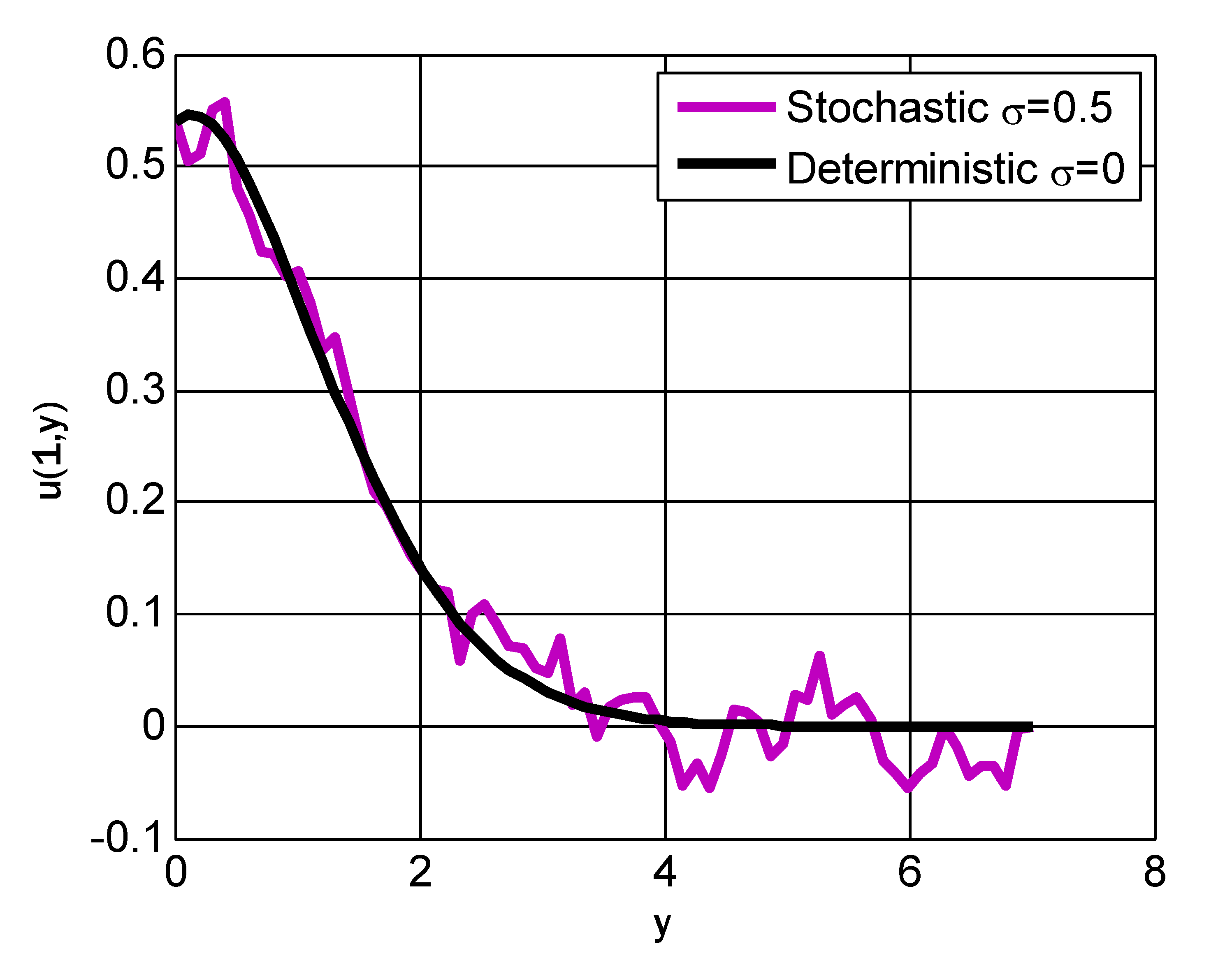
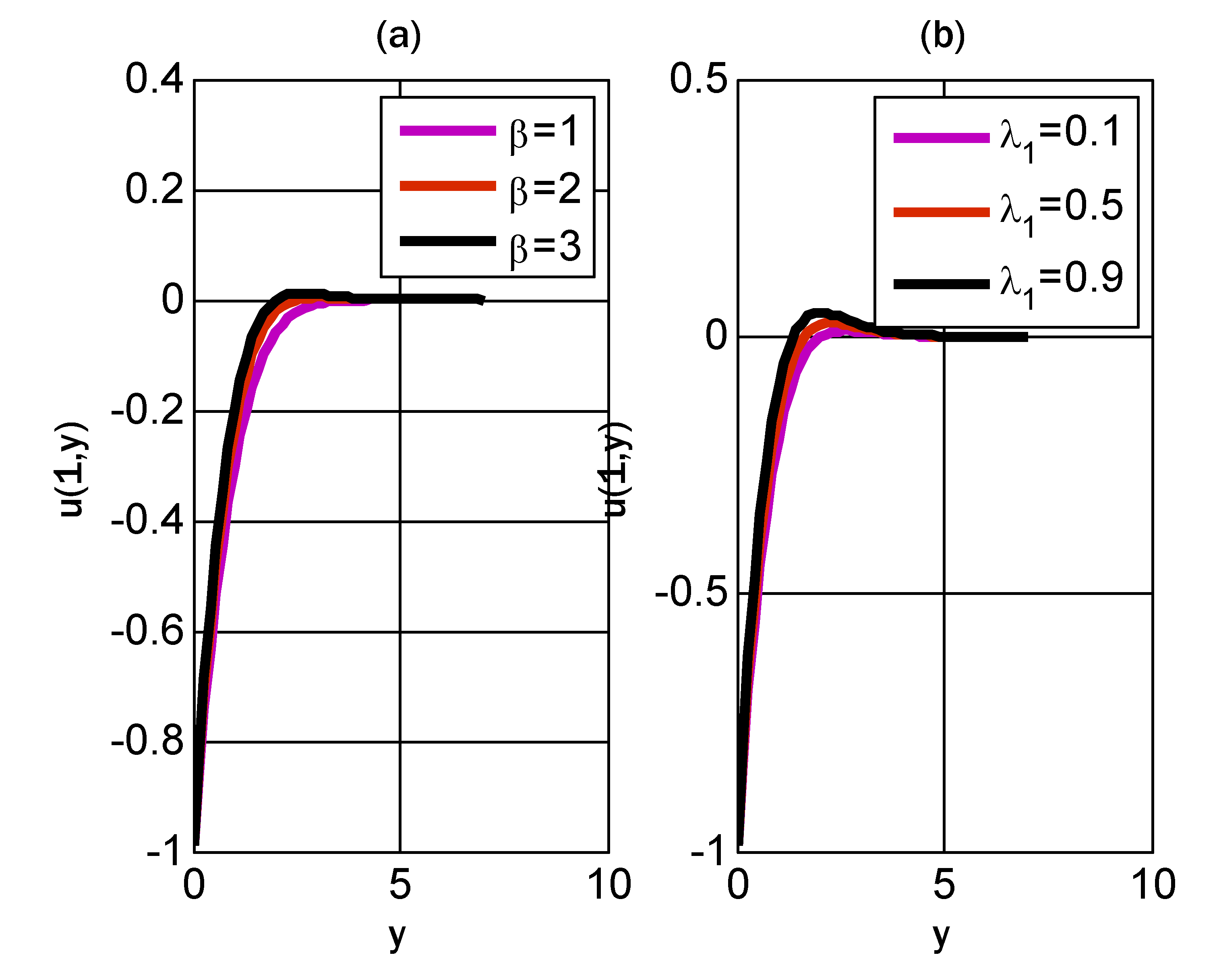
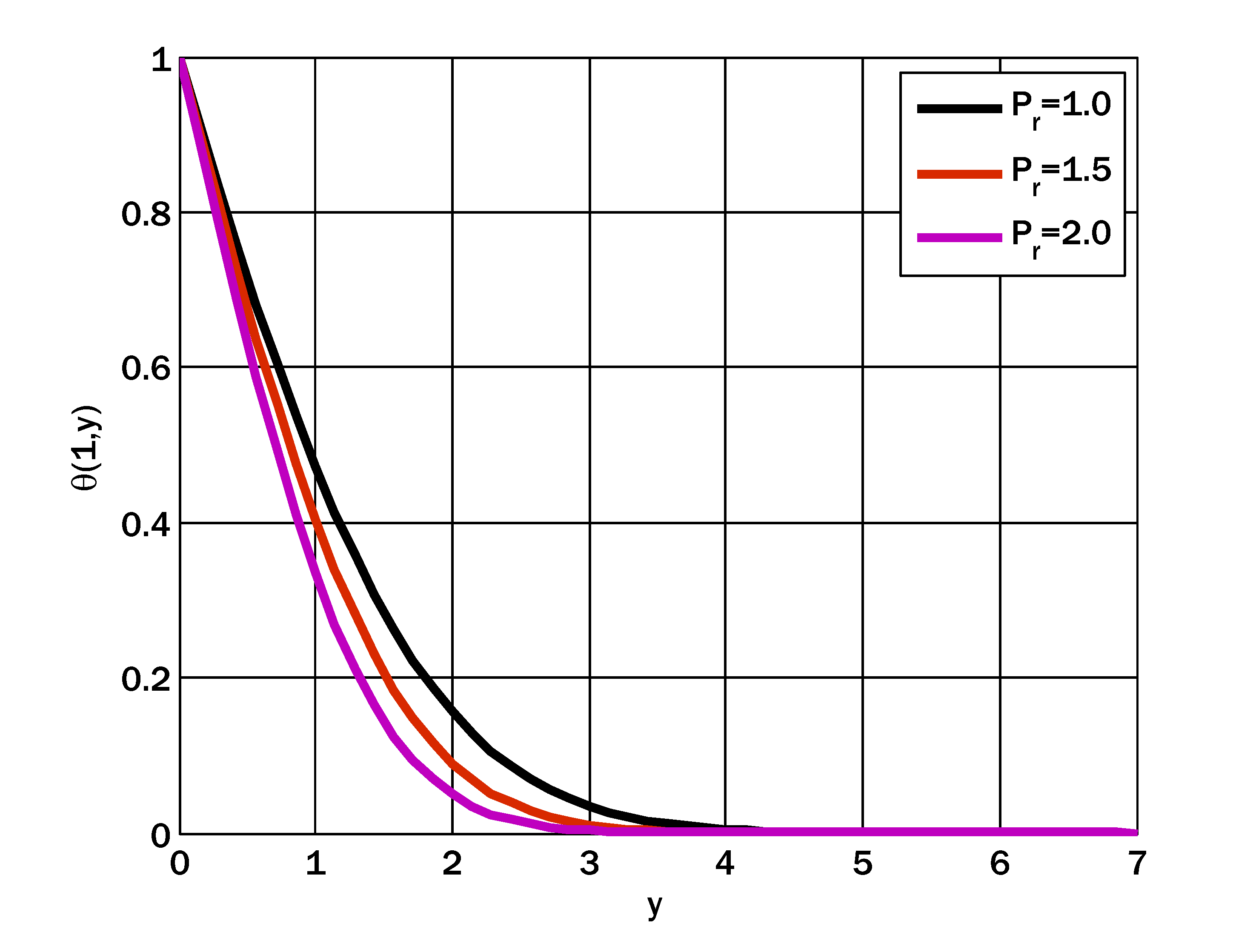
The correspondence between the deterministic and stochastic solutions is displayed in Figure 2. As mentioned earlier. The stochastic solution can be different on each code run, so the obtained solution is one of the possible stochastic solutions. The effect of Casson and mixed convection parameters on velocity is depicted in Figure 3. Figure 3 shows that the velocity profile has dual behavior by growing Casson and mixed convection parameters. The growth in the Casson parameter resulted from the decay in the diffusion coefficient, and consequently enhanced the velocity. The enhancement in the mixed convection parameter produced either decay in the viscosity of the fluid or growth in the temperature difference between the wall and the ambient fluid, and de-escalation of viscosity decreased the resistance to flow, so the fluid’s velocity increased. For mixed convective flow, the temperature gradient is one of the forces that enhances the fluid’s velocity, and therefore if the temperature increases, the velocity escalates. The effect of the thermophoresis parameter on the temperature profile is depicted in Figure 4. The temperature profile escalated by increasing that values of the thermophoresis parameter. By increasing the thermophoresis parameter, the thermophoresis force grew, which was responsible for late circulating the fluid’s particles near p, leading to enhancement in the temperature profile. Figure 5 depicts the effect of the Prandtl number on the temperature distribution. An increase in the Prandtl number caused a decreasing temperature profile. Reducing thermal conductivity and diffusivity due to a rising Prandtl number caused a downward shift in the temperature distribution.
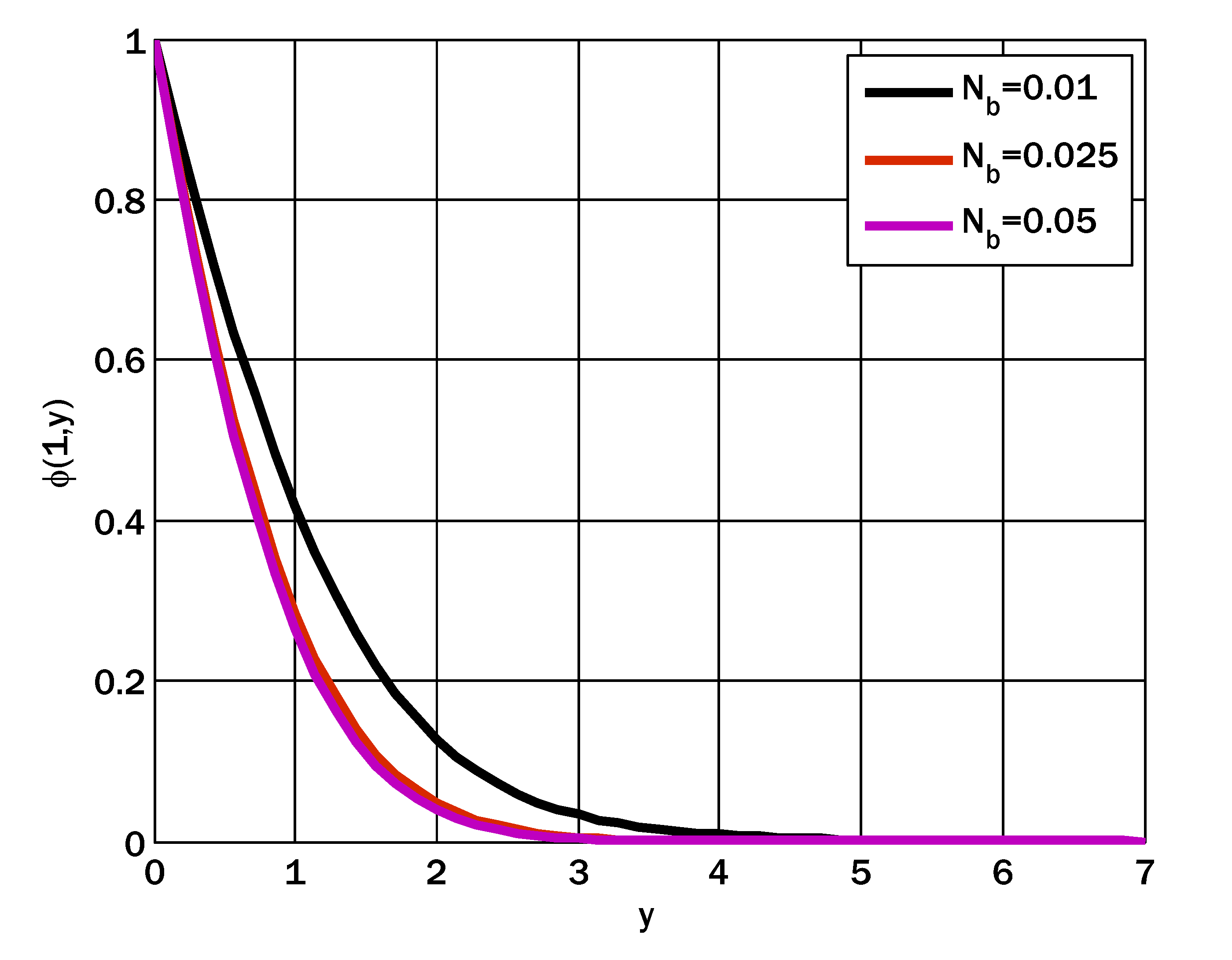
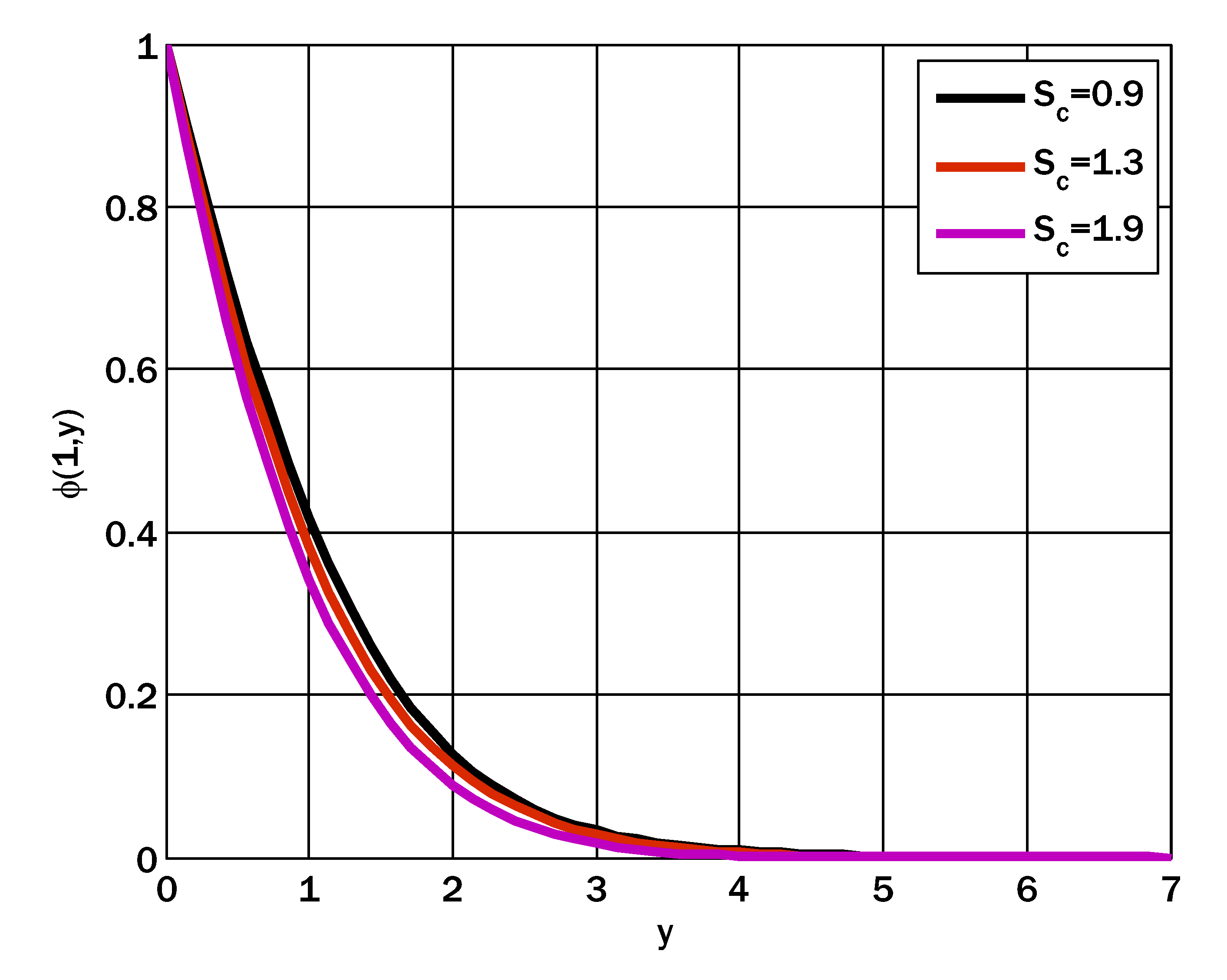
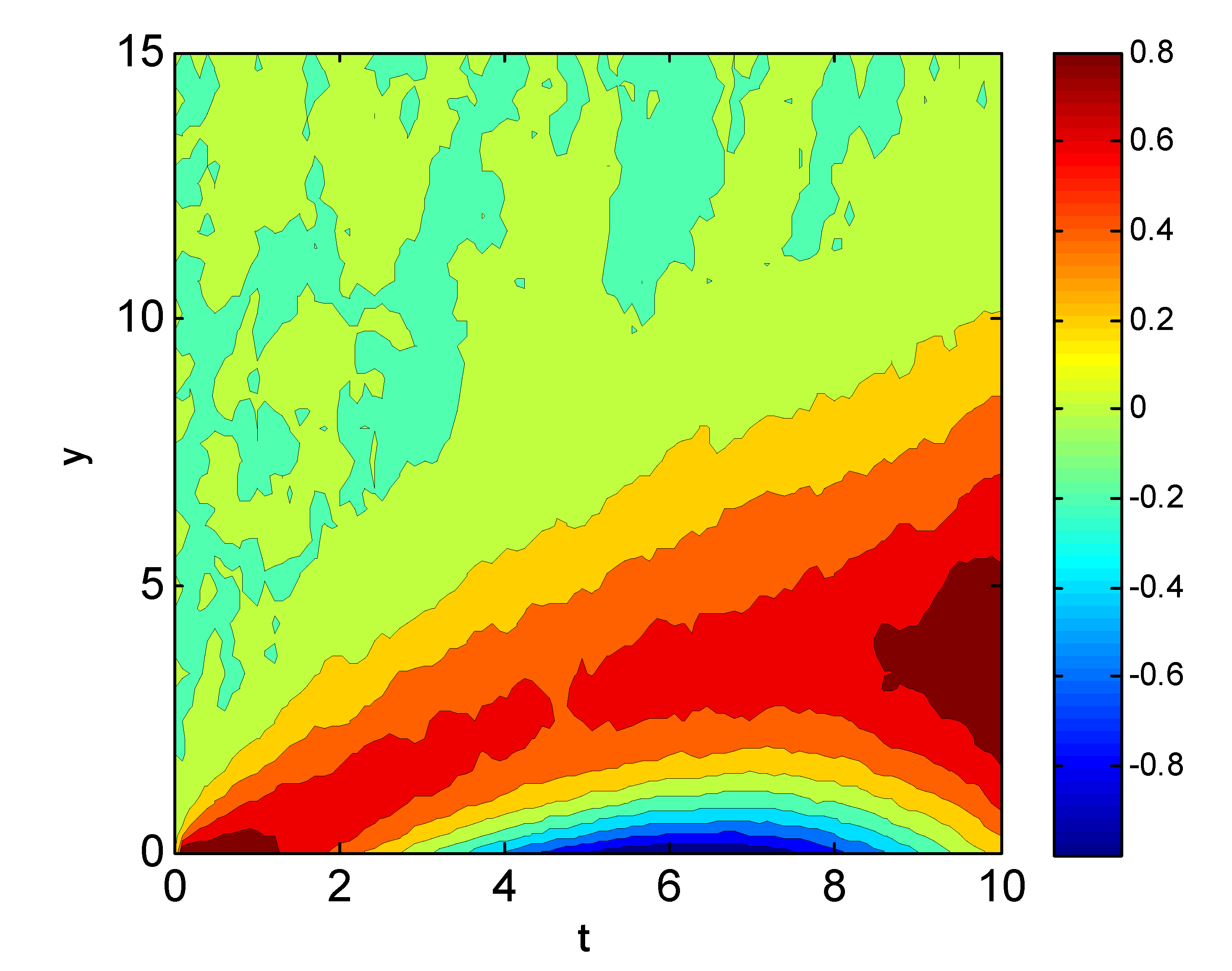
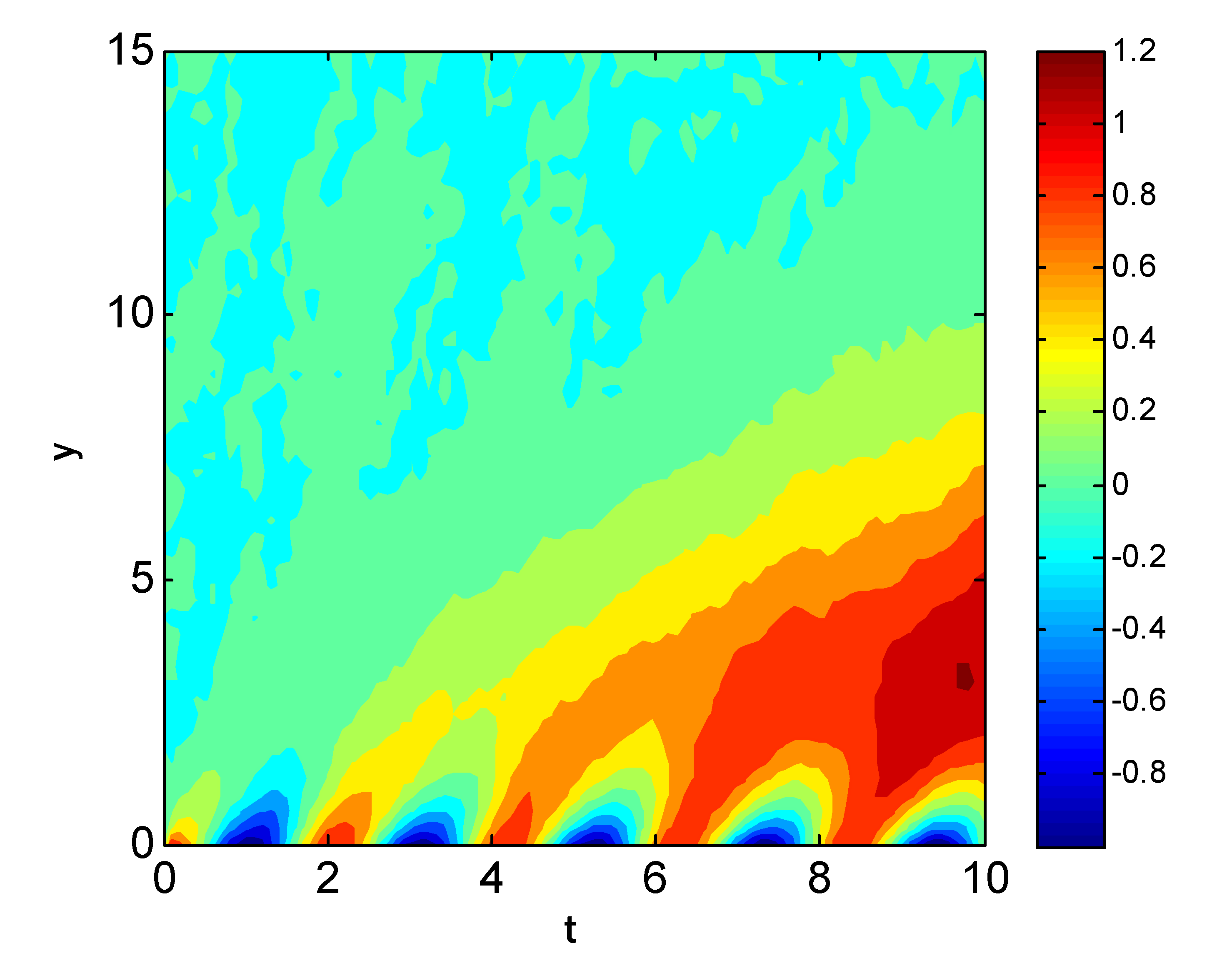
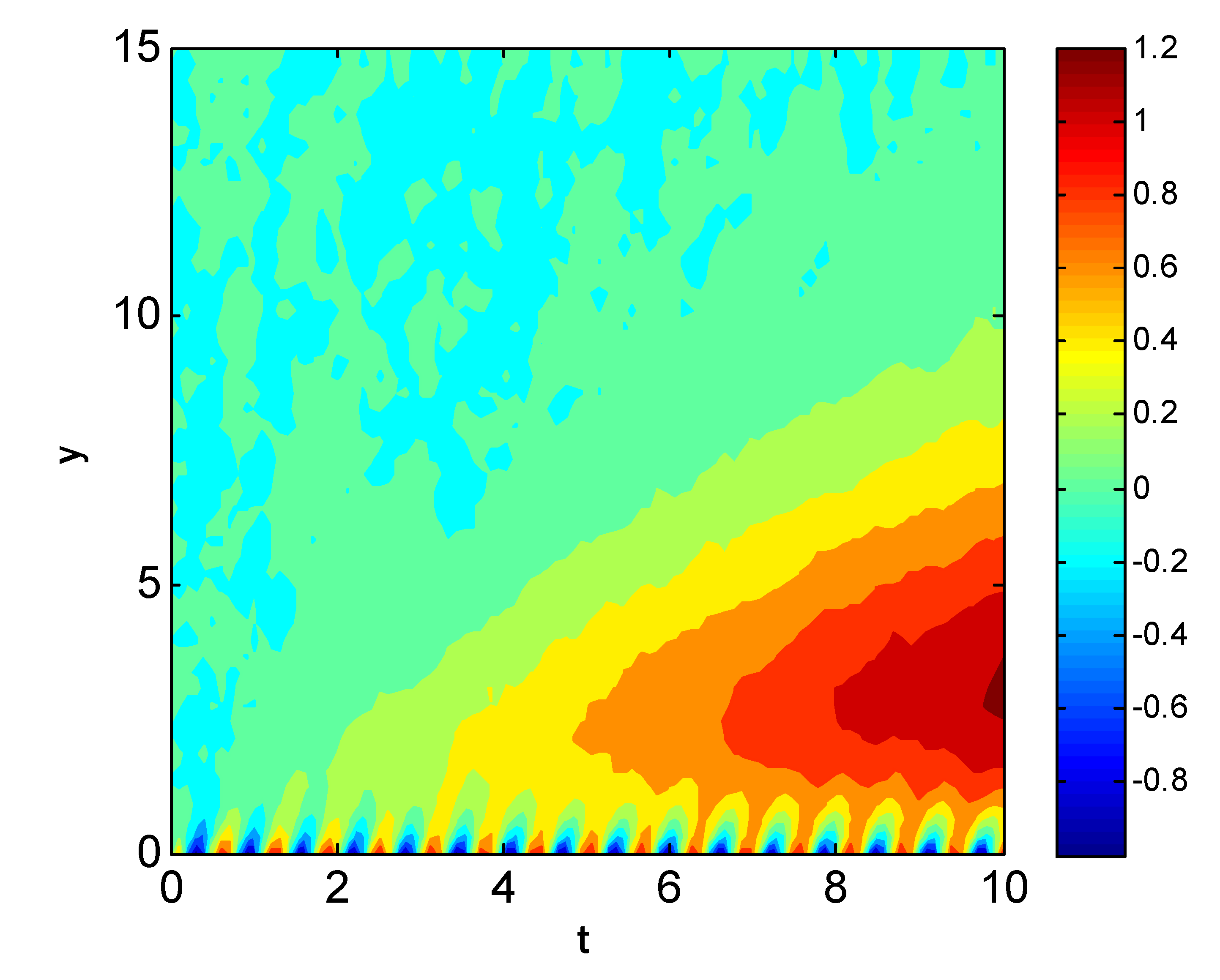
Figure 6 and Figure 7 exhibit concentration profiles as a function of Brownian motion and thermophoresis parameters. As the Brownian motion and thermophoresis parameters increased, the concentration profile decreased and expanded. Figure 8 depicts the effect of the Schmidt number on the concentration profile. The concentration profile declined with the increasing Schmidt number. Since mass diffusivity decays decreased by raising the Schmidt number, therefore the concentration profile declined. The influence of the dimensionless reaction rate parameter on the concentration profile is depicted in Figure 9. The concentration profile decreased by enhancing the reaction rate parameter. The concentration profile decreased as the development or dissolution of chemical bonds between atoms did not affect the nuclei. The contours for the velocity profile are displayed in Figure 10, Figure 11 and Figure 12, with varying periods of cosine boundary conditions. The height of the profiles in contour plots in Figure 10, Figure 11 and Figure 12 is described in the sidebar. Colors reflect the maximum to minimum profile heights. The contour plots represent the stochastic model’s solution, whereas Figure 3, Figure 4, Figure 5, Figure 6, Figure 7, Figure 8 and Figure 9 depict the deterministic model’s solutions.

7. Conclusions

This study comprised a numerical scheme for handling time-dependent stochastic partial differential equations (PDEs). The scheme was constructed on three time levels. At the first time level, the stochastic Crank–Nicolson scheme was utilized. The stability and consistency of the constructed scheme have been reported. A new and improved mathematical model of a non-Newtonian Casson nanofluid flow across an oscillatory sheet was presented. The model was reduced to a dimensionless stochastic partial differential equations (SPDEs) system. The current method can be used in other applications after completing this project [53,54,55,56,57]. The proposed method solves a wider variety of stochastic partial differential equations (SPDEs) and is straightforward to apply. The concluding points can be expressed as:
  • The velocity profile had dual behavior by incrementing Casson and mixed convection parameters.
  • The temperature profile was escalated by enhancing the thermophoresis parameter.
  • The concentration profile decayed and grew by increasing the Brownian motion and thermophoresis parameters, respectively.

Author Contributions

Conceptualization, methodology, and analysis, Y.N.; funding acquisition, K.A.; investigation, Y.N.; methodology, M.S.A.; project administration, K.A.; resources, K.A.; supervision, M.S.A.; visualization, K.A.; writing—review and editing, M.S.A.; proofreading and editing, M.S.A. All authors have read and agreed to the published version of the manuscript.

Funding

The authors would like to acknowledge the support of Prince Sultan University for paying the Article Processing Charges (APC) of this publication.

Data Availability Statement

The manuscript included all required data and implementing information.

Acknowledgments

The authors wish to express their gratitude to Prince Sultan University for facilitating the publication of this article through the Theoretical and Applied Sciences Lab.

Conflicts of Interest

The authors declare no conflict of interest.

References

  1. Simiu, E. Chaotic Transition in Deterministic and Stochastic Systems; Princeton University Press: Princeton, NJ, USA, 2002. [Google Scholar]
  2. Maciejewski, P.; Moffat, R. Heat Transfer with Very High Free-Stream Turbulence, Part I: Experimental Data. J. Heat Transf. 1992, 114, 827–833. [Google Scholar] [CrossRef]
  3. Lucor, D.; Karniadakis, G. Noisy Inflows Cause a Shedding Mode Switching in Flow Past an Oscillating Cylinder. Phys. Rev. Lett. 2004, 92, 154501. [Google Scholar] [CrossRef] [PubMed] [Green Version]
  4. Espanol, P.; Warren, P. Statistical Mechanics of Dissipative Particle Dynamics. Europhys. Lett. 1995, 30, 191–196. [Google Scholar] [CrossRef] [Green Version]
  5. Lou, Z.; Yang, W.J. A computer simulation of the non-Newtonian blood flow at the aortic bifurcation. J. Biomech. 1993, 26, 37–49. [Google Scholar] [CrossRef] [Green Version]
  6. Papanastasiou, T.C.; Boudouvis, A.G. Flows of viscoplastic materials: Models and computations. Comput. Struct. 1997, 64, 677–694. [Google Scholar] [CrossRef]
  7. Li, G.; Chen, B.; Zhou, G. Unsteady non-Newtonian solver on unstructured grid for the simulation of blood flow. Adv. Mech. Eng. 2013, 2013, 596172. [Google Scholar] [CrossRef]
  8. Venkatesan, J.; Sankar, D.; Hemalatha, K.; Yatim, Y. Mathematical analysis of Casson fluid model for blood rheology in stenosed narrow arteries. J. Appl. Math. 2013, 2013, 583809. [Google Scholar] [CrossRef] [Green Version]
  9. Amlimohamadi, H.; Akram, M.; Sadeghy, K. Flow of a Casson fluid through a locally constricted porous channel: A numerical study. Korea Aust. Rheol. J. 2016, 28, 129–137. [Google Scholar] [CrossRef]
  10. Makinde, O.D.; Sandeep, N.; Ajayi, T.; Animasaun, I.L. Numerical Exploration of Heat Transfer and Lorentz Force Effects on the Flow of MHD Casson Fluid over an Upper Horizontal Surface of a Thermally Stratified Melting Surface of a Paraboloid of Revolution. Int. J. Nonlinear Sci. Numer. Simul. 2016, 19, 93–106. [Google Scholar] [CrossRef]
  11. Thumma, T.; Wakif, A.; Animasaun, I.L. Generalized differential quadrature analysis of unsteady three-dimensional MHD radiating dissipative Casson fluid conveying tiny particles. Heat Transf. 2020, 49, 2595–2626. [Google Scholar] [CrossRef]
  12. Mahmood, R.; Kousar, N.; Usman, K.; Mehmood, A. Finite element simulations for stationary Bingham fluid flow past a circular cylinder. J. Braz. Soc. Mech. Sci. Eng. 2018, 40, 459. [Google Scholar] [CrossRef]
  13. Nawaz, Y.; Arif, M.S.; Abodayeh, K. An Unconditionally Stable Third Order Scheme for Mixed Convection Flow between Parallel Plates with Oscillatory Boundary Conditions; John Wiley and Sons Ltd.: Hoboken, NJ, USA, 2023. [Google Scholar] [CrossRef]
  14. Nawaz, Y.; Arif, M.S.; Abodayeh, K. Predictor–Corrector Scheme for Electrical Magnetohydrodynamic (MHD) Casson Nanofluid Flow: A Computational Study. Appl. Sci. 2023, 13, 1209. [Google Scholar] [CrossRef]
  15. Arif, M.S.; Abodayeh, K.; Nawaz, Y. The modified finite element method for heat and mass transfer of unsteady reacting flow with mixed convection. Front. Phys. 2022, 10, 802. [Google Scholar] [CrossRef]
  16. Shatnawi, T.A.M.; Abbas, N.; Shatanawi, W. Mathematical Analysis of Unsteady Stagnation Point Flow of Radiative Casson Hybrid Nanofluid Flow over a Vertical Riga Sheet. Mathematics 2022, 10, 3573. [Google Scholar] [CrossRef]
  17. Mehmood, A.; Mahmood, R.; Majeed, A.H.; Awan, F.J. Flow of the Bingham Papanastasiou Regularized Material in a Channel in the Presence of Obstacles: Correlation between Hydrodynamic Forces and Spacing of Obstacles. Model. Simul. Eng. 2021, 2021, 5583110. [Google Scholar] [CrossRef]
  18. Ilyas, H.; Ahmad, I.; Raja, M.A.Z.; Shoaib, M. A novel design of Gaussian wave nets for rotational hybrid nanofluidic flow over a stretching sheet involving thermal radiation. Int. Commun. Heat Mass Transf. 2021, 123, 105196. [Google Scholar] [CrossRef]
  19. Hamid, A.; Chu, Y.-M.; Khan, M.I.; Kumar, R.N.; Gowd, R.J.P.; Prasannakumara, B.C. Critical values in axisymmetric flow of magneto-cross nanomaterial towards a radially shrinking disk. Int. J. Mod. Phys. B 2021, 35, 2150105. [Google Scholar] [CrossRef]
  20. Hussain, S.; Tunç, O.; Rahman, G.U.; Khan, H.; Nadia, E. Mathematical analysis of stochastic epidemic model of MERS-corona & application of ergodic theory. Math. Comput. Simul. 2023, 207, 130–150. [Google Scholar] [CrossRef]
  21. Ahmad, I.; Raja, M.A.Z.; Ramos, H.; Bilal, M.; Shoaib, M. Integrated neuro-evolution-based computing solver for dynamics of non-linear corneal shape model numerically. Neural Comput. Appl. 2021, 33, 5753–5769. [Google Scholar] [CrossRef]
  22. Shatnawi, T.A.M.; Abbas, N.; Shatanawi, W. Comparative study of Casson hybrid nanofluid models with induced magnetic radiative flow over a vertical permeable exponentially stretching sheet. Am. Inst. Math. Sci. AIMS Math. 2022, 7, 20545–20564. [Google Scholar] [CrossRef]
  23. Shoaib, M.; Kausar, M.; Khan, M.I.; Zeb, M.; Gowda, R.P.; Prasannakumara, B.; Alzahrani, F.; Raja, M.A.Z. Intelligent backpropagated neural networks application on Darcy-Forchheimer ferrofluid slip flow system. Int. Commun. Heat Mass Transf. 2021, 129, 105730. [Google Scholar] [CrossRef]
  24. Hayat, T.; Khan, M.; Khan, M.I.; Alsaedi, A.; Ayub, M. Electromagneto squeezing rotational flow of carbon (C)-water (H2O) kerosene oil nanofluid past a Riga plate: A numerical study. PLoS ONE 2017, 12, e0180976. [Google Scholar] [CrossRef] [PubMed] [Green Version]
  25. Wakif, A.; Animasaun, I.; Sehaqui, R. A brief technical note on the onset of convection in a horizontal nanofluid layer of finite depth via Wakif-Galerkin weighted residuals technique (WGWRT). Defect Diffus. Forum 2021, 409, 90–94. [Google Scholar] [CrossRef]
  26. Shah, Z.; Raja, M.A.Z.; Chu, Y.-M.; Khan, W.A.; Waqas, M.; Shoaib, M.; Abbass, S.Z. Design of neural network based intelligent computing for neumerical treatment of unsteady 3D flow of Eyring-Powell magneto-nanofluidic model. J. Mater. Res. Technol. 2020, 9, 14372–14387. [Google Scholar] [CrossRef]
  27. Turkyilmazoglu, M. Unsteady mhd flow with variable viscosity: Applications of spectral scheme. Int. J. Therm. Sci. 2010, 49, 563–570. [Google Scholar] [CrossRef]
  28. Turkyilmazoglu, M. Effective Computation of Solutions for Non-linear Heat Transfer Problems in Fins. J. Heat Transfer. 2014, 136, 091901. [Google Scholar] [CrossRef]
  29. Turkyilmazoglu, M. Effective computation of exact and analytic approximate solutions to singular non-linear equations of Lane–Emden–Fowler type. Appl. Math. Model. 2013, 37, 7539–7548. [Google Scholar] [CrossRef]
  30. Turkyilmazoglu, M. Equivalence of ratio and residual approaches in the homotopy analysis method and some applications in non-linear science and engineering. Comput. Model. Eng. Sci. 2019, 120, 63–81. [Google Scholar]
  31. Iftikhar, B.; Javed, T.; Siddiqu, M.A. Entropy generation analysis during MHD mixed convection flow of non-Newtonian fluid saturated inside the square cavity. J. Comput. Sci. 2023, 66, 101907. [Google Scholar] [CrossRef]
  32. Harish, R.; Sivakumar, R. Effects of nanoparticle dispersion on turbulent mixed convection flows in cubical enclosure considering Brownian motion and thermophoresis. Powder Technol. 2021, 378, 303–316. [Google Scholar] [CrossRef]
  33. Abderrahmane, A.; Alqsair, U.F.; Guedri, K.; Jamshed, W.; Nasir, N.A.A.; Majdi, H.S.; Baghaei, S.; Mourad, A.; Marzouki, R. Analysis of mixed convection of a power-law non-Newtonian nanofluid through a vented enclosure with rotating cylinder under magnetic field. Ann. Nucl. Energy 2022, 178, 109339. [Google Scholar] [CrossRef]
  34. Hassan, A.; Hussain, A.; Arshad, M.; Awrejcewicz, J.; Pawlowski, W.; Alharbi, F.M.; Karamti, H. Heat and Mass Transport Analysis of MHD Rotating Hybrid Nanofluids Conveying Silver and Molybdenum Di-Sulfide Nano-Particles under Effect of Linear and Non-Linear Radiation. Energies 2022, 15, 6269. [Google Scholar] [CrossRef]
  35. Arshad, M.; Hussain, A.; Hassan, A.; Karamti, H.; Wróblewski, P.; Khan, I.; Andualem, M.; Galal, A.M. Scrutinization of Slip Due to Lateral Velocity on the Dynamics of Engine Oil Conveying Cupric and Alumina Nanoparticles Subject to Coriolis Force. Math. Probl. Eng. 2022, 2022, 2526951. [Google Scholar] [CrossRef]
  36. Tessitore, G. Existence, uniqueness and space regularity of the adapted solutions of a backward SPDE. Stoch. Anal. Appl. 1996, 14, 461–486. [Google Scholar] [CrossRef]
  37. Dozzi, M.; López-Mimbela, J.A. Finite-time blowup and existence of global positive solutions of a semilinear SPDE. Stoch. Process. Appl. 2010, 120, 767–776. [Google Scholar] [CrossRef] [Green Version]
  38. Xiong, J.; Yang, X. Existence and pathwise uniqueness to an SPDE driven by a-stable colored noise. Stoch. Process. Appl. 2019, 129, 2681–2722. [Google Scholar] [CrossRef]
  39. Altmeyer, R.; Bretschneider, T.; Janák, J.; Reiß, M. Parameter estimation in an SPDE model for cell repolarization SIAM/ASA. J. Uncertain. Quantif. 2022, 10, 179–199. [Google Scholar] [CrossRef]
  40. Gyöngy, I.; Martínez, T. On numerical solution of stochastic partial differential equations of elliptic type Sto-chastics: An International. J. Probab. Stoch. Process. 2006, 78, 213–231. [Google Scholar] [CrossRef]
  41. Kamrani, M.; Hosseini, S.M. The role of coefficients of a general SPDE on the stability and convergence of a finite difference method. J. Comput. Appl. Math. 2010, 234, 1426–1434. [Google Scholar] [CrossRef]
  42. Yasin, M.W.; Iqbal, M.S.; Ahmed, N.; Akgül, A.; Raza, A.; Rafiq, M.; Riaz, M.B. Numerical scheme and stability analysis of stochastic Fitzhugh-Nagumo model. Results Phys. 2022, 32, 105023. [Google Scholar] [CrossRef]
  43. Yasin, M.W.; Iqbal, M.S.; Seadawy, A.R.; Baber, M.Z.; Younis, M.; Rizvi, S.T. Numerical scheme and analytical solutions to the stochastic nonlinear advection diffusion dynamical model. Int. J. Nonlinear Sci. Numer. Simul. 2021. [Google Scholar] [CrossRef]
  44. Allen, E.J.; Novosel, S.J.; Zhang, Z. Finite element and difference approximation of some linear stochastic partial differential equations. Stoch. Int. J. Probab. Stoch. Process. 1998, 64, 117–142. [Google Scholar] [CrossRef]
  45. Kruse, R. Consistency and stability of a Milstein-Galerkin finite element scheme for semilinear SPDE. Stoch. Partial. Differ. Eq. Anal. Comput. 2014, 2, 471–516. [Google Scholar] [CrossRef] [Green Version]
  46. Roth, C. A combination of finite difference and Wong-Zakai methods for hyperbolic stochastic partial differential equations. Stoch. Anal. Appl. 2006, 24, 221–240. [Google Scholar] [CrossRef]
  47. Namjoo, M.; Mohebbian, A. Approximation of stochastic partial differential equations with stochastic crank-nicolson method. In Proceedings of the 21st Seminar on Mathematical Analysis and its Applications, Hamedan, Iran, 26–27 November 2014. [Google Scholar]
  48. Li, Y.; Mao, X.; Song, Q.; Wu, F.; Yin, G. Strong convergence of Euler-Maruyama schemes for McKean-Vlasov stochastic differential equations under local Lipschitz conditions of state variables IMA. J. Numer. Anal. 2022, 2022, 107. [Google Scholar] [CrossRef]
  49. Hu, L.; Li, X.; Mao, X. Convergence rate and stability of the truncated Euler-Maruyama method forstochastic differential equations. J. Comput. Appl. Math. 2018, 337, 274–289. [Google Scholar] [CrossRef]
  50. El-Metwally, H.; Sohaly, M.A.; Elbaz, I.M. Mean-square stability of the zero equilibrium of the nonlinear delay differential equation: Nicholson’s blowflies application. Nonlinear Dyn. 2021, 105, 1713–1722. [Google Scholar] [CrossRef]
  51. Mohammed, M. Well-Posedness for Non-linear Parabolic Stochastic Differential Equations with Non-linear Robin Conditions. Symmetry 2022, 14, 1722. [Google Scholar] [CrossRef]
  52. Ishfaq, N.; Khan, W.; Khan, Z. The Stokes’ second problem for nanofluids. J. King Saud Univ.-Sci. 2019, 31, 61–65. [Google Scholar] [CrossRef]
  53. Abodayeh, K.; Raza, A.; Arif, M.S.; Rafiq, M.; Bibi, M.; Fayyaz, R. Numerical analysis of stochastic vector borne plant disease model. Comput. Mater. Contin. 2020, 62, 65–83. [Google Scholar] [CrossRef]
  54. Arif, M.S.; Raza, A.; Shatanawi, W.; Rafiq, M.; Bibi, M. A stochastic numerical analysis for computer virus model with vertical transmission over the internet. Comput. Mater. Contin. 2019, 61, 1025–1043. [Google Scholar]
  55. Shatanawi, W.; Raza, A.; Arif, M.S.; Abodayeh, K.; Rafiq, M.; Bibi, M. Design of nonstandard computational method for stochastic susceptible–infected–treated–recovered dynamics of coronavirus model. Adv. Differ. Equ. 2020, 2020, 505. [Google Scholar] [CrossRef] [PubMed]
  56. Pasha, S.A.; Nawaz, Y.; Arif, M.S. The modified homotopy perturbation method with an auxiliary term for the non-linear oscillator with discontinuity. J. Low Freq. Noise Vib. Act. Control. 2019, 38, 1363–1373. [Google Scholar] [CrossRef] [Green Version]
  57. Bibi, M.; Nawaz, Y.; Arif, M.S.; Abbasi, J.N.; Javed, U.; Nazeer, A. A finite difference method and effective modification of gradient descent optimization algorithm for MHD fluid flow over a linearly stretching surface. Comput. Mater. Contin. 2020, 62, 657–677. [Google Scholar]
Figure 1. Geometry of the problem.
Energies 16 02298 g001
Figure 2. Deterministic and stochastic velocity profile using N t = 110 ,   N y = 70 ,   σ = 0.3 ,   β   λ 1 = 0 ,   λ 2 = 0 .
Energies 16 02298 g002
Figure 3. Deterministic variation of Casson and mixed convection parameters on the velocity profile using N t = 100 ,   N y = 50 ,   σ = 0 ,   P r = 0.9 ,   S c = 0.9 ,   γ = 0.1 ,   ε 1 = 0.1 ,   N t = 0.01 ,   N b = 0.01 ,   λ 2 = 0.1 ,   δ 1 = 0.1 ,   δ 2 = 0.1   (a) λ 1 = 0.1   (b) β = 3 .
Energies 16 02298 g003
Figure 4. Deterministic variation of the thermophoresis parameter on the temperature profile using N t = 100 ,   N y = 50 ,   σ = 0 ,   P r = 0.9 ,   S c = 0.9 ,   γ = 0.1 ,   ε 1 = 0.1 ,   N t = 0.01 ,   N b = 0.01 ,   λ 2 = 0.1 ,   δ 1 = 0.1 ,   δ 2 = 0.1 ,   λ 1 = 0.1 , β = 3 .
Energies 16 02298 g004
Figure 5. Deterministic variation of the Prandtl number on the temperature profile using N t = 100 ,   N y = 50 ,   σ = 0 ,   S c = 0.9 ,   γ = 0.1 ,   ε 1 = 0.1 ,   N t = 0.01 ,   N b = 0.01 ,   λ 2 = 0.1 ,   δ 1 = 0.1 ,   δ 2 = 0.1 ,   λ 1 = 0.1 ,   β = 3 .
Energies 16 02298 g005
Figure 6. Deterministic variation of the Brownian motion parameter on the concentration profile using N t = 100 ,   N y = 50 ,   σ = 0 ,   P r = 0.9 ,   S c = 0.9 ,   γ = 0.1 ,   ε 1 = 0.1 ,   N t = 0.01 ,   λ 2 = 0.1 ,   δ 1 = 0.1 ,   δ 2 = 0.1 ,   λ 1 = 0.5 ,   β = 3 .
Energies 16 02298 g006
Figure 7. Deterministic variation of the thermophoresis parameter on the concentration profile using N t = 100 ,   N y = 50 ,   σ = 0 ,   P r = 0.9 ,   S c = 0.9 ,   γ = 0.1 ,   ε 1 = 0.1 ,   N b = 0.01 ,   λ 2 = 0.1 ,   δ 1 = 0.1 ,   δ 2 = 0.1 ,   λ 1 = 0.5 ,   β = 3 .
Energies 16 02298 g007
Figure 8. Deterministic variation of the Schmidt number on the concentration profile using N t = 100 ,   N y = 50 ,   σ = 0 ,   P r = 0.9 ,   N t = 0.01 ,   γ = 0.1 ,   ε 1 = 0.1 ,   N b = 0.01 ,   λ 2 = 0.1 ,   δ 1 = 0.1 ,   δ 2 = 0.1 ,   λ 1 = 0.5 ,   β = 3 .
Energies 16 02298 g008
Figure 9. Deterministic variation of the reaction rate parameter on the concentration profile using N t = 100 ,   N y = 50 ,   σ = 0 ,   P r = 0.9 ,   N t = 0.01 ,   S c = 0.9 ,   ε 1 = 0.1 ,   N b = 0.01 ,   λ 2 = 0.1 ,   δ 1 = 0.1 ,   δ 2 = 0.1 ,   λ 1 = 0.5 ,   β = 3 .
Energies 16 02298 g009
Figure 10. Stochastic contours of the velocity profile using N t = 100 ,   N y = 50 ,   σ = 0.15 ,   P r = 0.9 ,   N t = 0.01 ,   S c = 0.9 ,   ε 1 = 0.1 ,   N b = 0.025 ,   λ 2 = 0.1 ,   δ 1 = 0.1 ,   δ 2 = 0.1 ,   λ 1 = 0.5 ,   β = 3 ,   γ = 0.1 ,   U w = c o s 0.5 t .
Energies 16 02298 g010
Figure 11. Stochastic contours of the velocity profile using N t = 100 ,   N y = 50 ,   σ = 0.15 ,   P r = 0.9 ,   N t = 0.01 ,   S c = 0.9 ,   ε 1 = 0.1 ,   N b = 0.025 ,   λ 2 = 0.1 ,   δ 1 = 0.1 ,   δ 2 = 0.1 ,   λ 1 = 0.5 ,   β = 3 ,   γ = 0.1 ,   U w = c o s 3 t .
Energies 16 02298 g011
Figure 12. Stochastic contours of the velocity profile using N t = 100 ,   N y = 50 ,   σ = 0.15 ,   P r = 0.9 ,   N t = 0.01 ,   S c = 0.9 ,   ε 1 = 0.1 ,   N b = 0.025 ,   λ 2 = 0.1 ,   δ 1 = 0.1 ,   δ 2 = 0.1 ,   λ 1 = 0.5 ,   β = 3 ,   γ = 0.1 ,   U w = c o s 10 t .
Energies 16 02298 g012
Disclaimer/Publisher’s Note: The statements, opinions and data contained in all publications are solely those of the individual author(s) and contributor(s) and not of MDPI and/or the editor(s). MDPI and/or the editor(s) disclaim responsibility for any injury to people or property resulting from any ideas, methods, instructions or products referred to in the content.