Wellbore and Reservoir Thermodynamic Appraisal in Acid Gas Injection for EOR Operations

Abstract

This study provides insights into the experience gained from investigating the thermodynamic behavior of well and reservoir fluids during acid gas injection (AGI) in a hydrocarbon field to enhance oil recovery (EOR) and to reduce greenhouse gas emissions. Unlike conventional water and natural gas injection, AGI involves complicated phase changes and physical property variations of the acid gas and reservoir fluids at various pressure-temperature (P-T) conditions and compositions, and both constitute crucial parts of the EOR chain. A workflow is developed to deal with the reservoir fluid and acid gas thermodynamics, which is a key requirement for a successful design and operation. The workflow focuses firstly on the development of the thermodynamic models (EoS) to simulate the behavior of the reservoir fluids and of the injected acid gas and their integration in the field and in well dynamic models. Subsequently, the workflow proposes the thermodynamic simulation of the fluids’ interaction to determine the Minimum Miscibility Pressure (MMP), yielding the dynamic evolution of the fluids’ miscibility that may appear within the reservoir. Flow assurance in the acid gas transportation lines and in the wellbore is also considered by estimating the hydrate formation conditions.

1. Introduction

Sour resources are hydrocarbon reservoirs that contain a significant amount of H₂S and, potentially, a smaller amount of CO₂, which have to be removed at gas plants before the treated gas is consumed on-site or forwarded to the sales line [1,2]. For that purpose, produced sour gas is processed (“sweetened”) by separating its H₂S and/or CO₂ content in amine units to give a natural gas product with specifications appropriate for transport to a variety of end users. Traditionally, the resulting acid gas waste stream (primarily comprising H₂S and CO₂) is processed in sulphur recovery units (SRUs), such as the Claus unit, which convert H₂S to elemental sulphur [2,3]. However, SRUs are not a major revenue generator, due to the economically unattractive sulphur market price, and are primarily installed for environmental purposes. Furthermore, air emission standards and regulatory authorities are becoming increasingly stringent, thereby increasing the economical strain on oil and gas companies, which are in search of environment-friendly and cost-effective alternative methods for dealing with acid gases produced in association with sour natural resources [1].

One such alternative is acid gas injection (AGI) into the appropriate subsurface reservoirs, combining operating expenses cuts due to the Claus unit deactivation, reduced sulphur emissions into the atmosphere, and increased oil recovery [2]. Acid gas is composed mainly of H₂S and/or CO₂, water vapor (arriving from the sour gas sweetening process), and other contaminants including methane and heavier hydrocarbons [4]. In basic AGI schemes (Figure 1), the produced sour gas undergoes a one or two-stage absorbing process where the sour gas stream comes into contact with an amine solution. After the removal of H₂S and CO₂ from the sour gas, the water-saturated acid gas mixture is separated from the amine unit at low pressures (35 to 70 kPa) and at relatively high temperatures, and is typically compressed in three or four stages to obtain sufficient pressure for its injection into the subsurface formation [5,6]. High-pressure acid gas flows through pipelines to the well site, arrives at the wellbore in a dense-fluid (liquid or supercritical) state, and finally gets injected into the reservoir through the well tubing [6]. Depending on the composition and the specifications set by the operator, it may also be necessary to dehydrate the acid gas to ensure a hydrate-free flow inside the pipeline and the wellhead as well as moderate corrosion [7].

As the global energy community progressively switches to less carbon and/or H₂S intensive greenhouse gas emissions, the number and size of AGI facilities progressively increases [8,9], as evidenced by the successful development of several previous and ongoing AGI projects. Sour/acid gas injection for storage or for EOR purposes has been the driving force behind some of these developments, and has provided the industry with significant experience in successfully transporting and injecting sour or acid gas [3]. The first, but rather small, AGI scheme was that by Chevron at Acheson, near Edmonton, Canada, that was initiated in 1989 [10]. Larger schemes followed, such as the AGI projects at Sleipner West in the North Sea, In-Salah in Algeria, and LaBarge in Wyoming, USA [7]. Besides those sites where the sour and acid gas mixtures injection is a common practice [11,12], AGI is now applied to many sour oil and gas reservoirs worldwide, such as the North Caspian basin (Tengiz field, Kazakhstan) [13,14,15] and the Middle East [16,17,18].

To run engineering calculations and to take financial decisions prior to the application of highly complex EOR projects, it is crucial to ensure that the thermodynamic models developed for the injected and reservoir fluids are able to deliver stable and valid results in the entire range of possible input parameter changes, such as P-T conditions and composition. Indeed, the comprehensive thermodynamic modelling of both acid gas and reservoir fluid constitutes a crucial part of the AGI design, since the models developed are incorporated into the integrated dynamic flow model used to evaluate the behavior of the entire system (reservoir-to-surface), whether AGI takes place in a pilot phase or full-scale simulation and, consequently, to conduct a cost-benefit analysis of the entire operation.

Although there is strong research interest in the industry concerning AGI technology, most of that is focused on the well and reservoir phenomena taking place, lacking expertise when it comes to fluid phase behavior and clearly explained, ready-to-use thermodynamic tools. In this work, we offer a fully detailed workflow that can be combined with any available commercial software in the industry and which can be fully applicable in relevant projects by supporting all aspects of thermodynamic calculations involved in AGI projects. In this work, we propose a workflow (Figure 2) that can be used to run a complete study of the reservoir/wellbore fluids thermodynamic behavior modelling during AGI for EOR operations. This is a very crucial procedure, especially in cases where limited information is available for the fluids involved (acid gas thermodynamics and its interaction with reservoir oil), and it provides a way for the initial assessment of the performance of a pilot AGI scheme. The workflow can be divided into four parts: (1) development of the thermodynamic models (EoS) for simulating the behavior of the acid gas followed by that of the reservoir fluid, (2) investigation of the acid gas conditions prevailing all along the well tubing (injection profiles), (3) the study of the interaction of the acid gas with the reservoir fluid to establish miscibility conditions, and (4) dealing with flow assurance issues that may occur due to the prevailing conditions (e.g., hydrates). The proposed workflow is applied to study the possibility of acid gas injection for EOR purposes in the ‘’Prinos’’ reservoir located in Northern Greece.

The rest of the paper is organized as follows: Section 2 discusses all thermodynamic modelling techniques needed for the setup and the evaluation of reservoir and acid gas fluid models. Section 3 studies the changes in phase behavior and properties resulting from changes in the operating conditions, mainly P-T, within the wellbore (injection profiles), and Section 4 presents the MMP estimation methodologies for the thermodynamic simulation of the interaction of acid gas and reservoir fluids to yield the dynamic evolution of the fluids’ miscibility within the reservoir. Section 5 focuses on the evaluation of flow assurance risks by predicting any possible event of hydrate formation. Finally, the results from the application of the developed workflow to the ‘’Prinos’’ reservoir are presented in Section 6. The paper concludes in Section 7.

2. Acid Gas and Reservoir Oil Thermodynamic Models

In this section, we demonstrate the methodology to develop all necessary computational tools needed to predict the thermodynamic properties of the fluids involved in the AGI process design. Clearly, a simplistic model based on the black oil principle cannot capture the complex thermodynamic effects taking place when fluid miscibility is considered, as in this case the displacement process strongly depends on pressure and fluid composition. As a result, all hydrocarbon phases should be treated as n_c-component mixtures and thus use an EoS component-based model instead.

Since all commercial reservoir and wellbore simulators only allow the use of one model per region to describe the thermodynamic behavior of the involved fluids, the single EoS model built must be compatible both with the reservoir oil and the acid gas phase behavior, in order for all future AGI simulations required for the full development of the AGI process to be accurate and successful.

Developing a common EoS model for multiple fluids is a challenging task, and needs to be addressed in a two-step approach. Firstly, the acid gas thermodynamic model (EoS) is developed in order to secure its functionality on acid gas components solely. The model can be built using the Peng-Robinson (PR) cubic EoS, since it is known to perform accurately when describing petroleum fluids and is supported by all commercial simulation software. The presence of polar components, such as brine or H₂S, requires a thorough investigation of the molecular interaction parameters to ensure the selected EoS performance.

As a next step, the EoS model developed for the acid gas must be extended to handle the reservoir fluid by applying pseudoization and the necessary splitting and lumping schemes of the heavy fraction. To build an EoS that is applicable to both fluids, its tunable parameters must be adjusted to match the available experimental data using regression, while at the same time, the acid gas ones are kept intact so as to retain their prediction accuracy with regard to the thermodynamic properties of the acid gas.

2.1. Acid Gas Thermodynamic Modelling

The acid gas phase behavior (single-phase liquid, single-phase gas, liquid-gas mixture, supercritical fluid) and its thermophysical properties must be accurately modelled over the entire range of P-T conditions prevailing along its journey from the amines unit outlet to the reservoir. To ensure that the parameters of the EoS used to characterize acid gas components are set accurately, the developed EoS is checked against available acid gas experimental data to validate its performance when reproducing phase saturation and density at various conditions of interest.

The Peng & Robinson cubic EoS (1978) is quite popular in oil and natural gas systems modelling in the petroleum industry, combining simplicity and low computational overhead [19]. It has been shown to accurately describe the phase equilibria of multiphase hydrocarbon mixtures at various P-T conditions and to provide reliable estimates of gas and liquid saturated volumes. The PR EoS has the following form:

$$P=\frac{RT}{V-b}-\frac{a}{V\left(V+b\right)+b\left(V+b\right)}$$

(1)

where $P$ is pressure, $T$ is temperature, and $V$ is the molar volume. Parameters $a$ and $b$ correspond to the attractive and repulsive forces effects, respectively, and are functions of the components’ properties and of their concentration.

To achieve accurate performance for the acid gas, the Binary Interaction Coefficients (BICs or k_ij), which enter as a corrective term in the mixing rule for the molecular attraction parameter, $a$, need to be set. The BIC of the H₂S-CO₂ pair is described by their average value of 0.095, as proposed by Chapoy et al. [20], whereas for the BICs of H₂S and CO₂ with H₂O, fixed predetermined values or, alternatively, zero ones may be used. It is worthy of note that this choice is not expected to affect the models, since the percentage of water in such mixtures is extremely low. Regarding the H₂S molar volume correction factor, a value of −0.10356, as proposed by Stamatakis and Magoulas [21], is recommended. The critical properties involved in the EoS are retained in their lab values, whereas the acentric factor is estimated by the Soave approach [22].

The evaluation of the predictions provided by the proposed acid gas thermodynamic model is accomplished by checking (1) vapor pressure and (2) density predictions on various experimental acid gas data collected from the literature. Regarding the first part, phase diagrams (or P-T diagrams) are the tool to check phase changes, as they depict the type and number of phases of the fluid under consideration at various P-T conditions. For pure components, such diagrams simplify to a simple line that delineates the region of pure liquid from that of the pure gas phase, while for mixtures of two or more components, it is an envelope that demarcates the two-phase from the single-phase region (gas or liquid) of acid gas. To evaluate the P-T diagrams produced by the thermodynamic model, they are compared against available experimental data. It must be noted that the toxicity of H₂S has only resulted in a limited number of studies containing acid gas saturation data. The experimental data obtained is presented in Section 6.2.

For the second part, density is a property of major importance because of its direct correlation with the hydrostatic head developed inside the injection well; hence, it must be determined with accuracy. Similar to the saturation conditions, the accuracy of the density predictions is based on their comparison with the experimental data that is presented in Section 6.2.

The aforementioned guidelines have shown to lead to a very accurate acid gas EoS model, as will be shown in the results section. Nevertheless, it should be remembered that although more accurate models are available in the thermodynamics community (such as the CPA one [23]), AGI process modelling is restricted by the commercial simulators which require that the fluid models need to be cubic EoS ones.

2.2. Reservoir Fluid Thermodynamic Modelling

To build the reservoir fluid thermodynamic model, the selected EoS developed for the acid gas needs to be extended, tuned, and evaluated to accurately predict the thermodynamic properties of the reservoir fluid as well. It is important that the EoS must be modified and tuned only on the basis of the hydrocarbon components of the reservoir fluid so as to retain its performance on the acid ones.

As a first step, all laboratory data about the reservoir fluid, including Compositional Analysis (CA), Constant Composition Expansion (CCE), Differential Liberation Expansion (DLE), and Lab Separation (LS) tests must be collected and quality controlled before being used as inputs to the thermodynamic model tuning. The EoS build process that follows incorporates the grouping and the initial characterization of the reservoir fluid components, the characterization of the heavy-end fraction (C_n+) and its splitting and lumping into pseudo-components, and the determination of the BICs and of the molar volume correction factors to accurately estimate the saturated volumes of the liquid phase.

To optimally reproduce the experimental data, regression of the tunable parameters, such as the critical pressure (P_c) and critical temperature (T_c) of the heavier pseudo-components, is required for the EoS model to match the data. As the reservoirs selected to undergo a miscibility injection typically lie at pressures above the saturation one, the test data of immediate interest are the volumetric properties of the fluid at saturation, i.e., B_o, R_s, and oil density at that pressure. Similarly, since AGI for EOR is applied to oil reservoirs that have undergone primary (depletion) and possibly secondary (i.e., water-flooding) production, the production is driven by oil compressibility, which also needs to be estimated accurately. This requirement becomes significant when considering that pressure change above the saturation one is strongly related to compressibility, since it is easy to show that:

$$\Delta P=\frac{1}{c}ln\left(\frac{\rho }{{\rho }_0}\right)$$

(2)

From Equation (2), it follows that the lower the oil compressibility, the lower the density change. Therefore, when the fluid is subjected to a pressure increase ΔP, the latter is dominated by the compressibility value, an accurate estimate of which is required.

The EoS model needs to be tuned against surface data (GOR, API) as well, in order to avoid misleadingly accurate pressure-volume predictions due to volume error cancellation. Moreover, accurate reproduction of the surface data is a must when the EoS model is utilized in order to generate a black oil equivalent one (e.g., in WinProp, 2022 software [24]), [25] which in turn is incorporated into a black oil simulator to speed up the matching step. At this point it must be noted that when more than one fluid is present in a reservoir, the EoS tuning process must be repeated for each fluid separately.

For the EoS to be tailored for a specific multi-component system, proper characterization of the components of the reservoir mixture is required, especially of the heavy-end (C_n+), and particularly the determination of their critical properties (T_c, P_c), acentric factor (ω), and the volume translation parameter (V_s). The splitting and lumping of the C_n+ is an important process that is required to obtain a representative description of the fluid, and is usually performed using the Pedersen [26] or the Whitson methodology, since a detailed SCN analysis is very rare [27]. The obtained lumped pseudos are characterized by using empirical correlations, which are functions of their molecular weight and specific gravity. The splitting process focuses on two criteria: (1) the accurate reproduction of the experimental data, and (2) the optimization of the total number of components of the mixture, since the higher the number of components, the larger the computational time requirement.

The BICs account for the interactions between each pair of components of the mixture, and are of great importance when there are significant differences in the size and type of the molecules, and when in the presence of non-hydrocarbons such as CO₂, H₂S, and N₂. The Prausnitz correlation is commonly used to set the BICs of the HCs-HCs binary systems [28], and is defined by

$$k_{ij}=1-{\left(\frac{2V_{ci}^{\raisebox{1ex}{$1$}\!\left/ \!\raisebox{-1ex}{$6$}\right.} V_{cj}^{\raisebox{1ex}{$1$}\!\left/ \!\raisebox{-1ex}{$6$}\right.}}{V_{ci}^{\raisebox{1ex}{$1$}\!\left/ \!\raisebox{-1ex}{$3$}\right.}+V_{ci}^{\raisebox{1ex}{$1$}\!\left/ \!\raisebox{-1ex}{$3$}\right.}}\right)}^{\theta }$$

(3)

where V_ci and V_cj are the critical volumes of components i and j respectively, and θ, which is usually set to 1.2, is the HC—HC interaction coefficient exponent.

For the CO₂-HCs pairs above methane, correlations from standard engineering textbooks can be used [22]. Since H₂S presence is crucial in the studied mixtures, a dedicated solution is preferred for the H₂S-HCs pairs. The following generalized correlation of Stamataki & Magoulas (2000), [21] has shown satisfying accuracy

$$k_{ij}=0.1029-0.1498\omega$$

(4)

where $\omega$ is the acentric factor of each pairing component. For the CO₂-CH₄ pair, the following method is recommended

$$k_{ij}=a\left({\omega }_j\right)+b\left({\omega }_j\right)T_{ri}+c\left({\omega }_j\right)T_{ri}^3$$

(5)

and appears in Kordas, Tsoutsouras, Stamataki, & Tassios (1994) [29]. This correlation is suitable in the case of n-alkanes. The $a$, $b$, and $c$ parameters are quadratic functions of the HC component acentric factor. For the case of methane, the method provides a value of $k_{ij}=0.105$.

The liquid phase molar volumes, as obtained by the PR EoS, show significant deviation from their exact values and, thus, their accurate calculation requires the use of specialized correction relations, such as the Volume Shift technique. The volume translation relation of Jhaveri and Youngren [30], especially for the case of the pseudo-components, is recommended in order to obtain decent predictions of the liquid phase saturated volume.

Once completed, the characterization of the mixture’s components is used as the input to the EoS model tuning process, where it is possible to further adjust the developed EoS, accurately reproduce the available experimental data, and simulate the phase behavior of the reservoir oil. Despite the fact that there is no single standard tuning technique, those approaches typically aim at minimizing the sum of weighted squared deviations between the lab measurements and the EoS estimates by tuning the uncertain parameters (i.e., pseudo-components’ properties). Weights, which are associated with single pressure steps or groups of steps, assign a degree of importance to each data point.

3. Specification of the Gas Injection Conditions

The second item in the proposed workflow is the investigation of the prevailing conditions (P-T) along the injection well. This is a subject of major interest for the design of the injection well itself and of the surface equipment in order to ensure two tasks, (1) single-phase state flow (liquid or supercritical) of the acid gas inside the well, and (2) that the acid gas will reach the well bottom in a supercritical state and at sufficient pressure to achieve full miscibility with the reservoir fluid.

For the first task, depending on the prevailing conditions, the acid gas may undergo phase changes at the wellhead, lengthwise, and at the bottom of the well. These changes depend on a combination of the P-T conditions, phase behavior, friction pressure loss, gravity effects, and heat exchange with the formation, and may lead to unusual operating characteristics and hazards within the well if not handled. Pipe erosion is probably the most notorious issue, as it may lead to the need to fully replace the tubing string. Among the critical parameters that can affect the acid gas phase behavior is its composition, as it is directly related to phase change limits (i.e., the phase envelope [31]) and the gas density, which in turn controls the hydrostatic pressure gain. Another critical parameter is the injection rate, which directly controls the friction pressure loss. In conjunction with the injection temperature at the wellhead, and the thermal conductivity between the tubing and the surrounding environment of the well, the heat exchange between the injected fluid and the individual parts of the well is also considered. This, in turn, controls the prevailing temperature, which, similarly to pressure, indirectly affects the phase change and pressure loss due to the effect of temperature on density and viscosity. It should be noted that when considering acid gas at supercritical conditions, its density, hence gravitational effects, is very sensitive to temperature changes.

To demonstrate the complexity and interdependence of the aforementioned critical parameters that can affect the acid gas behavior, we note that at low injection rates, the flow velocity is low, as sufficient time is provided for the acid gas to exchange heat with the formation. Thus, as acid gas flows toward the bottom of the well, its temperature will quickly converge to that of the formation until they become identical. If the flow rate and/or the thermal resistance to heat transfer between the formation and the well are high, the heat exchange between the acid gas and the formation is minimized so that the flow can be considered approximately adiabatic (negligible rate of heat exchange with the surroundings) and the acid gas temperature can remain significantly lower than the formation one, as it is not sufficiently heated.

The basic tool to study phase changes is the generation and evaluation of acid gas P-T conditions as a function of the depth (length) of the injection well, also known as the injection profile. To generate a well profile, one needs to start from the boundary pressure and temperature at the wellhead and integrate the pressure differential all along the well, i.e.,

$$P\left(D\right)={{\displaystyle \int }}_0^P\frac{dP}{dL}dL$$

(6)

where $\frac{dP}{dL}={\left(\frac{dP}{dL}\left(\rho \right)\right)}_g+{\left(\frac{dP}{dL}\left(\mu \right)\right)}_f+{\left(\frac{dP}{dL}\right)}_m$, the three terms of which account for pressure loss due to gravity, friction and momentum, or fluid acceleration. Complex effects such as heat transfer, slip hold, and two-phase flow regimes (if needed) are incorporated into the density and viscosity and to the friction factor appearing indirectly in ${\left(\frac{dP}{dL}\right)}_f$.

Injection profiles can be used to examine the effect of various critical parameters, such as the gas pressure and temperature at the wellhead, its composition, the injection rate, etc. To examine the effect of those crucial, and at the same time uncertain, parameters, a sensitivity analysis must be run to establish whether, and to what extent, they could affect the fluids’ behavior in the well. The sensitivity analysis method recommended is the “one at a time” approach, and it aims at varying one input parameter (one factor at a time—OFAT) and examining its effect in the final result. More specifically, it includes the following steps: (1) the definition of a base case scenario which incorporates the best estimates of the parameters involved according to the available knowledge, (2) the perturbation of an input parameter, within limits, while keeping all other values constant at their initial value according to the base case scenario, and (3) the reset of this parameter to its original value and repeat of the process for the next input parameter. This sensitivity analysis will reveal the possibly strong effect of each uncertain parameter on the well profile, and thus it will shed light on those which might violate the single-phase flow constraint.

For the second task, to ensure the smooth miscibility of the acid gas with the existing oil within the reservoir, it is necessary to estimate the minimum required wellhead injection pressure ($P_{wh}^{Inj}$). This pressure is of great importance in the design of the AGI operation, since it is a key factor for determining the amount of horsepower requirements for gas compression [32]. A reverse calculation procedure is followed to determine this value, which starts from the reservoir and develops in a reverse mode towards the wellhead, as can be seen in Figure 3.

To ensure full miscibility, the prevailing pressure at each point within the reservoir between the injecting and producing wells needs to be higher than the MMP, noted by $P^{MMP}$. Given the uncertainty of the MMP estimate (see next section), a safety margin $\Delta P^{MMP}$ is set so that the pressure within the reservoir should exceed the combined limit of $P^{MMP}+\Delta P^{MMP}$. The minimum pressure inside the reservoir is expected to occur at the bottom of the production well due to drawdown inside the formation during flow. Therefore

$$P_{wf}^{Prod}\ge P^{MMP}+\Delta P^{MMP}$$

(7)

where $P_{wf}^{Prod}$ represents the bottomhole pressure of the production well under flowing conditions. The bottomhole pressure of the injection well ($P_{wf}^{Inj}$) should be sufficiently high to anticipate the pressure loss, $\Delta P_{res}$, within the formation. This condition is ensured by

$$P_{wf}^{Inj}\ge P_{wf}^{Prod}+\Delta P_{res}=P^{MMP}+\Delta P^{MMP}+\Delta P_{res}$$

(8)

Finally, the required injection pressure at the wellhead, $P_{wh}^{Inj}$, is determined by additionally taking into account the pressure loss, $\Delta P^{Inj}$, along the AGI well, so that

$$P_{wh}^{Inj}=P_{wf}^{Inj}+\Delta P^{Inj}\ge P^{MMP}+\Delta P^{MMP}+\Delta P_{res}+\Delta P^{Inj}$$

(9)

Unlike conventional production wells, when injecting there is a gain of pressure during the flow of acid gas from the wellhead to the well bottom as the effect of gravity prevails over that of friction. To maintain the simplicity of mathematical expressions, a negative sign is placed before the term $\Delta P^{Inj}$, while the term itself is set to positive at its absolute value. Based on the above, the finally obtained minimum required $P_{wh}^{Inj}$ is given by

$$P_{wh}^{Inj}\ge P^{MMP}+\Delta P^{MMP}+\Delta P_{res}-\Delta P^{Inj}$$

(10)

It is therefore made clear that in order to successfully determine the minimum required wellhead pressure, the pressure difference inside the wellbore, $\Delta P^{Inj}$, should be first calculated and evaluated through the generation of the injection profiles.

4. MMP Estimation Methodologies

The next workflow item in which thermodynamic properties are involved is the mixing of the acid gas with the existing reservoir fluid to achieve miscibility. Acid gas mixing leads to a dramatic change in the reservoir oil properties, causing its swelling, and consequently changing its density (oil lightens) and viscosity (oil viscosity decreases), hence its mobility. A particularly important property is the Minimum Miscibility Pressure (MMP), the value of which is directly related to the required injection pressure at the wellhead, as discussed in Section 3. Formally, MMP is defined as the minimum pressure at which the injected gas and oil within the reservoir are completely mixed at any ratio into a homogeneous phase, without the existence of an interface.

If no laboratory measurements (typically in special PVT analysis) are available, MMP can be determined (a) by using established MMP correlations for H₂S-rich systems, (b) by simulating the slim tube experiment, (c) by using the cell-to-cell computational method, and (d) by exploiting reliable experimental measurements collected from the literature on fluids with a composition similar to that of the fluids of interest (analogs).

The MMP estimation using literature correlations, developed for combinations of reservoir fluids with acid gas, may have limited applicability due to the limited number of models applicable to H₂S-rich gases. In fact, most correlations available have been developed for CO₂-rich gases, as CO₂ is the commonly used agent in miscibility projects. Nevertheless, CO₂-oriented correlations which further take into account the presence of H₂S can still be utilized. Of course, the estimates resulting from such correlations can only be considered indicative and can only be used for an initial appraisal. Since H₂S is treated as an impurity rather than the abundant component, the MMP estimates obtained are expected to be higher than their actual values, as H₂S is known to have a beneficial (reducing) effect on the MMP value.

Various computational methods have been developed in recent years aiming to suppress the cost and time requirements of experimental methods. Routine and special PVT experimental procedures can now be simulated provided that the phase behavior of fluids can be accurately described by means of an EoS model. One such method is the simulation of the slim tube laboratory experiment, which is typically run to estimate the MMP by evaluating the oil recovery factor after a specific acid gas volume is injected at various pressures. In its simulating replicate, the simulator solves the one-dimensional flow equation using the common EoS of the reservoir fluid and of the injected gas which travels through the porous medium. Rock properties are only assigned typical values, as they do not affect the phase behavior phenomena which take place; however, a very well-tuned EoS is necessary to optimally describe the phase behavior of the fluids.

According to the cell-to-cell method, single-phase reservoir fluid at reservoir temperature is continuously enriched by mixing it with acid gas until the oil becomes saturated and a second phase appears, i.e., no more acid gas can be dissolved in the oil. The pressure is then increased and the process is repeated with fresh oil and fresh acid gas until a single phase is observed for any trial mixing ratio, which marks that the test pressure is the first contact MMP. Additionally, the cell-to-cell procedure can be used to estimate forward contacts MMP by following the same strategy until an unstable mixture is obtained. The mixture is then flashed at the current pressure, the equilibrium oil is enriched with more acid gas, and the process is repeated. If the procedure ends up at a single phase point, the prevailing pressure is the forward contacts MMP. Similarly, backward contacts MMP can be obtained by flashing the two-phase mixture, while mixing the equilibrium gas with fresh oil and repeating the procedure until a stable point is obtained, or the process arrives at a dead end (no more change in the equilibrium phases). Although this process can be run at the lab using physical acid gas and reservoir oil samples, it is typically run in a PVT simulation environment using the thermodynamic EoS model that describes both fluids [34].

A complementary evaluation of the above methods can be run using MMP experimental values obtained from the literature for combinations of reservoir fluids and injected gas, similar to those of the fluids of interest (analogs). Special attention should be paid to the “translation’’ of the similarity by considering the physical interpretation of each input parameter difference to the MMP. For example, increasing temperature between the case under study and its analog implies that the studied system’s MMP is expected to be higher than that of the analog, as temperature does not favor miscibility. Similarly, an increasing H₂S content in the acid gas as well as an increasing amount of the intermediate hydrocarbons lead to an MMP decrease, whereas the presence of methane in the agent gas causes its rapid increase.

5. Wellbore Flow Assurance

Since both CO₂ and H₂S are molecules that can be trapped in hydrate structures at conditions close to those expected in the AGI application, the estimation of hydrate formation pressure and temperature is required to ensure acid gas flow conditions within the wellbore that will prevent such a possibility.

Clathrate hydrates, simply known as gas hydrates, are solid solutions of hydrogen-bonded cavities of water molecules in which small gas molecules are trapped [35,36,37]. Typically, gas molecules are encapsulated in the hydrate cavities, whose structural stability depends on the Van der Waals and London forces generated by the interactions between the guest and host molecules [38]. Depending on the size of the guest molecules, three hydrate structures are known to form: structures I (sI), II (sII), and H (sH) [39,40]. The required conditions for their formation are a sufficient supply of gas and water under suitable p-T conditions [41,42]. The p-T phase envelope, also known as the hydrate equilibrium curve, defines the boundary line below which (i.e., at lower temperatures or at higher pressures) hydrates might form.

Although hydrates are a potential commodity and a promising energy technology for the future, they also pose a threat of severe plugging problems in the AGI context [43]. The standard industry practice is to mitigate hydrate formation risk by a continuous injection of thermodynamic hydrate inhibitors (THIs) [44]. Although THIs constitute an effective solution for shifting the hydrate equilibrium curve towards lower temperatures and/or higher pressures [45], this technique involves significant operational cost overheads to the pipeline network operators. As a result, practical solutions to reduce the amount of inhibitors while keeping the facility risk-free are an absolute necessity. The simplest way to reduce the inhibitor quantity is to avoid overdosing by perfectly matching the inhibitor concentration with the required level of inhibition, plus a marginal safety limit. For this task, accurate predictions of the hydrate formation p-T conditions obtained by accurate thermodynamic models must be used for the design of the inhibition strategy.

In order to assess the hydrate formation conditions, the formation curves can be obtained by means of commercial software such as HydraFLASH [46], Multiflash [47], etc., which first need to be validated against available experimental data on similar acid gas mixtures.

6. Results

6.1. AGI in “Prinos” Reservoir

The application of AGI for EOR purposes using the developed workflow is investigated for the “Prinos” complex located in the Prinos–Kavala offshore basin in the North Aegean Sea area of Greece, a tectonic rift created during the post-Alpine period (Figure 4). The field comprises the “Prinos”, “Epsilon” and “Prinos North” reservoirs 8 km west of the island of Thasos and 18 km south of the main coastline of Kavala in Greece, in a water depth of 30 to 38 m [48,49].

The “Prinos” reservoir is the main structure in the basin, and is formed by a fault-bounded low-relief anticline, with oil trapped at depths between 2490 m and 2790 m TVDSS. Facilities offshore and onshore allow the production of up to 30,000 barrels of oil per day (bbl/day). The offshore facilities are connected through a pipeline to the shore, where the natural gas and oil processing facilities are located, with oil storage tanks and an offshore loading terminal. The reservoir produces sour crude oil with an API between 27 and 30 degrees and a sour gas phase that contains up to 60% H₂S, as well as large amounts of CO₂. After being treated in the amines unit, the H₂S-free sweetened gas is used for energy and operational needs (gas lift). The design of the AGI scheme includes the redirection of the acid gas straight to the compressor instead of the Claus unit, through the seabed pipeline and eventually to the offshore site and into the injection well.

The acid gas composition under this study, or else the fluid of interest in the proposed workflow, is determined through a series of simulations based on the production forecast of the “Prinos” field. The runs simulate the complete surface processing system of the produced multiphase sour stream. Initially, reservoir streams collected from all wells are gathered in a common processing separator unit located offshore, where the resulting separated sour gas stream (Stream 1), along with the sour oil, is directed to the onshore processing unit. Onshore, the sour oil passes through a second separation unit, resulting in a new sour gas stream (Stream 2) and a liquid stream that is directed to the final oil stabilization unit. From the stabilization unit, the final liquid oil product is produced, along with a final sour gas stream (Stream 3). The three sour gas streams enter the amines unit where the resulting acid gas stream is produced.

For the acid gas injection rate, based on the operator’s production and composition forecast from the main processing units (first separator on the platform, second separator and stabilization units onshore), an estimation of the volume of the acid gas resulting from the amines was made. The acid gas volumes were estimated based on three envisaged field production scenarios corresponding to the minimum, average and the maximum supply of acid gas. It must be noted that acid gas recycling within the reservoir leads to cumulatively increasing the production of large acid gas volumes that will be constantly added to the injected stream. To account for that effect, the injection rate considered in the proposed workflow is set at three times the calculated maximum value, thus emulating a 30% acid gas loss in the reservoir and full recycling of the remaining 70%. Following the same reasoning, the most likely acid gas composition that was considered is the one that corresponds to the maximum acid gas rate.

6.2. Evaluation of the Thermodynamic Tools

6.2.1. Evaluation of the Acid Gas EoS Model

As discussed in Section 2, the evaluation of the predictions provided by the developed acid gas thermodynamic model is accomplished by comparing the vapor pressure and density predictions against experimental data on acid gas mixtures collected from the literature. The evaluation was run using the Absolute Average Relative Deviation formula

$$AARD\%=\frac{100}{N}{\displaystyle \sum }_{i=1}^N\frac{\left|{\rho }_i-{\widehat{\rho }}_i\right|}{{\rho }_i}$$

(11)

where ${\rho }_i$ is the experimental value, ${\widehat{\rho }}_i$ is the model estimated value, and $N$ is the number of experimental points considered.

Regarding the first part, Figure 5 illustrates the P-T diagrams as obtained from the experimental data of Bierlein [51], Kellerman [52] and Bennion [53] on top of the computationally obtained ones using the acid gas EoS model. Although the accuracy of the EoS was examined for all available experimental data, only a few phase envelopes are presented, covering a significant range of H₂S, CO₂ and CH₄ content, in order to demonstrate the results.

Clearly, the vapor pressure of pure H₂S, CO₂ and of all mixtures is accurately estimated by the thermodynamic model, as the observed deviations move within a tolerance margin of a few psi’s and °F. More specifically, the maximum deviation of lab data vapor pressure is in all cases less than 30 psi, with an average value of 18.5 psi (average absolute relative deviation of 1.8%). Hence, it can be concluded that the developed EoS model provides reliable P-T diagrams on all acid gas mixtures, even in the presence of low methane contamination.

Regarding acid gas density, the literature survey on the experimental acid gas density data leads to the work by Goodwin for pure H₂S [54], to three binary mixtures: (H₂S-CO₂) one from Kellerman [52] and two from Commodore [55], and a multicomponent system (H₂S-CO₂-CH₄) from Bennion [53]. The predictions of the developed thermodynamic model are shown in Figure 6 against the collected experimental data. The accuracy of the EoS model was examined for all available experimental density data in a manner similar to the process used for vapor pressure. For the sake of simplicity, only one dataset is presented as corresponding to the most similar composition to the fluid of interest. The densities of H₂S mixtures are estimated very accurately, as the observed deviations vary within the allowed tolerance margin. More specifically, the average absolute relative deviation of the experimental data density values is 1.1% for the case of 20 °C, and 4.9% for the case of 80 °C. In sum, it can be safely concluded that the developed EoS model for the acid gas provides reliable density estimates, thus guaranteeing accurate pressure gain calculations in the wellbore.

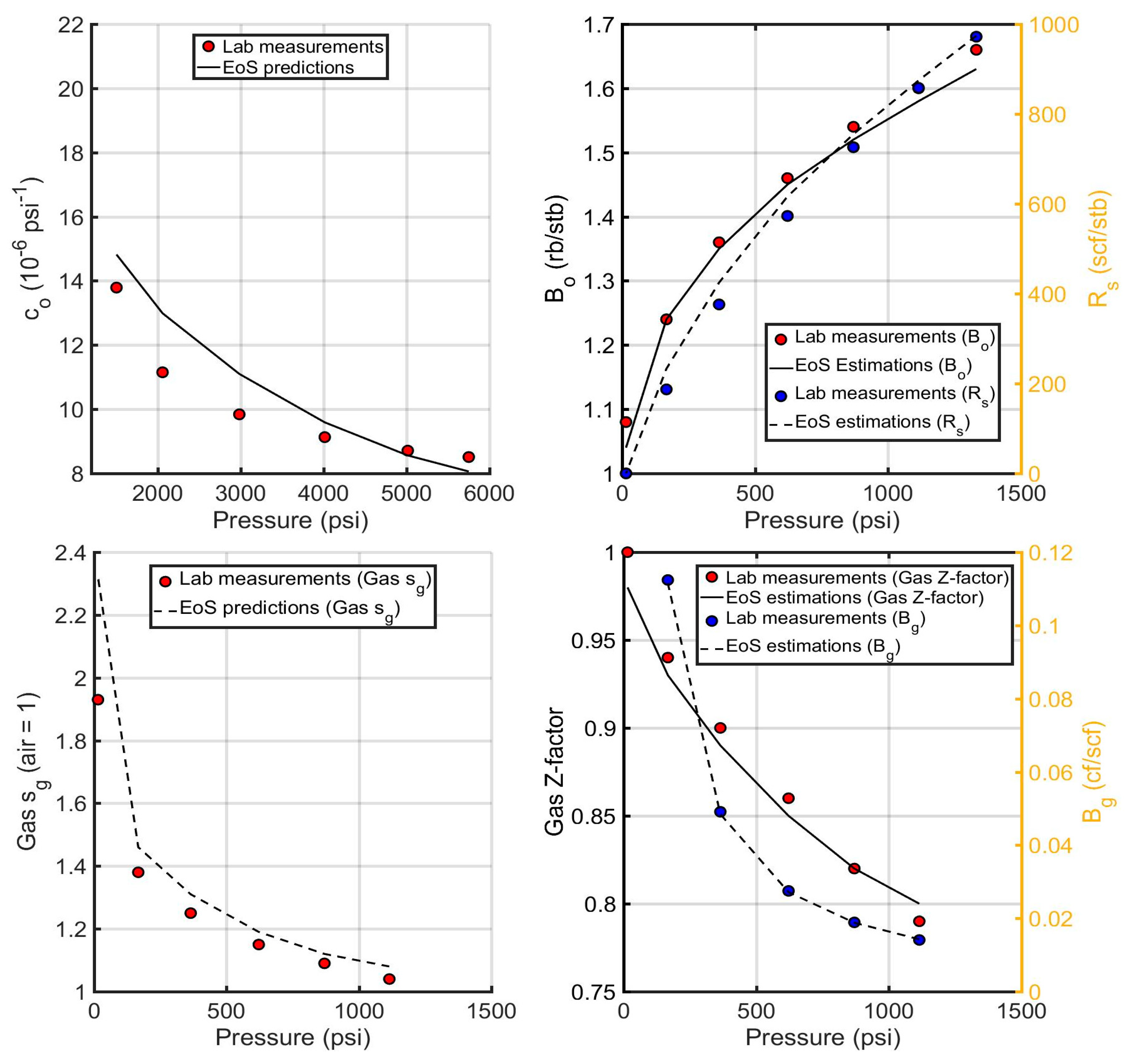
6.2.2. Evaluation of the Reservoir oil EoS Model

Following the two criteria proposed in Section 2 (the prediction accuracy of the experimental data and the optimization of the total number of components), the acid gas EoS model was extended by adding the hydrocarbon components, grouping them, and treating the heavy-end by splitting the C_n+ into three pseudo components (F₁, F₂, F₃). Nitrogen was grouped with methane as its initial concentration is insignificant, whereas C₄ and C₅ isomers were combined into two more components, thus leading to an 11-component EoS model.

When routine PVT study simulations were carried out to verify the ability of the model to accurately reproduce the available experimental data, the need to tune the EoS by regression analysis emerged. The parameters tuned were the critical properties (P_c, T_c), the acentric factors, the volume shift parameters of the three pseudos, as well as the BICs of each of these pseudo-components with CH₄ and H₂S, respectively, in an attempt to achieve matching with saturation pressure and experimental CCE and DLE test data.

Figure 7 illustrates the comparison between the volumetric properties estimates of the tuned PR EoS against the experimental CCE and DLE data. The simulation results of the CCE experiment under constant temperature, and more specifically the fluids’ compressibility in the single-phase region of the reservoir oil (top left side), produced a very small error (an AARD of approximately 6%), resulting in its satisfactory prediction. When simulating the DLE test, the pressure gradually decreases from the saturation pressure down to the atmospheric one. The B_o prediction proved to be excellent over the entire pressure range of the two-phase region, and the same is the case with the dissolved gas ratio (R_s) and gas formation volume factor (B_g) over the entire pressure range of the two-phase region, with an AARD value of less than 4%. Finally, the gas compressibility factor (Z factor) and gas specific gravity are reproduced with similar accuracy, although those values will not be utilized throughout the life of the reservoir, as the latter is undersaturated.

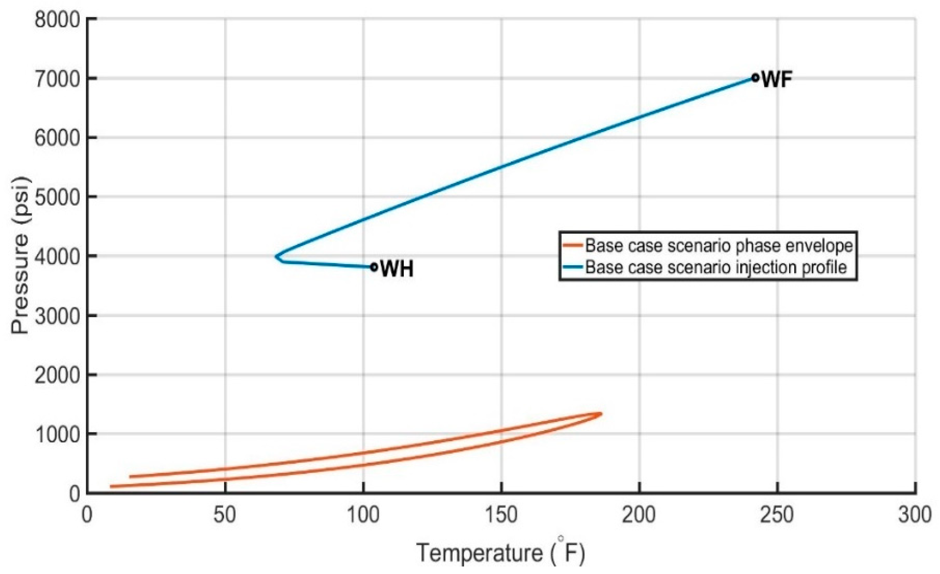
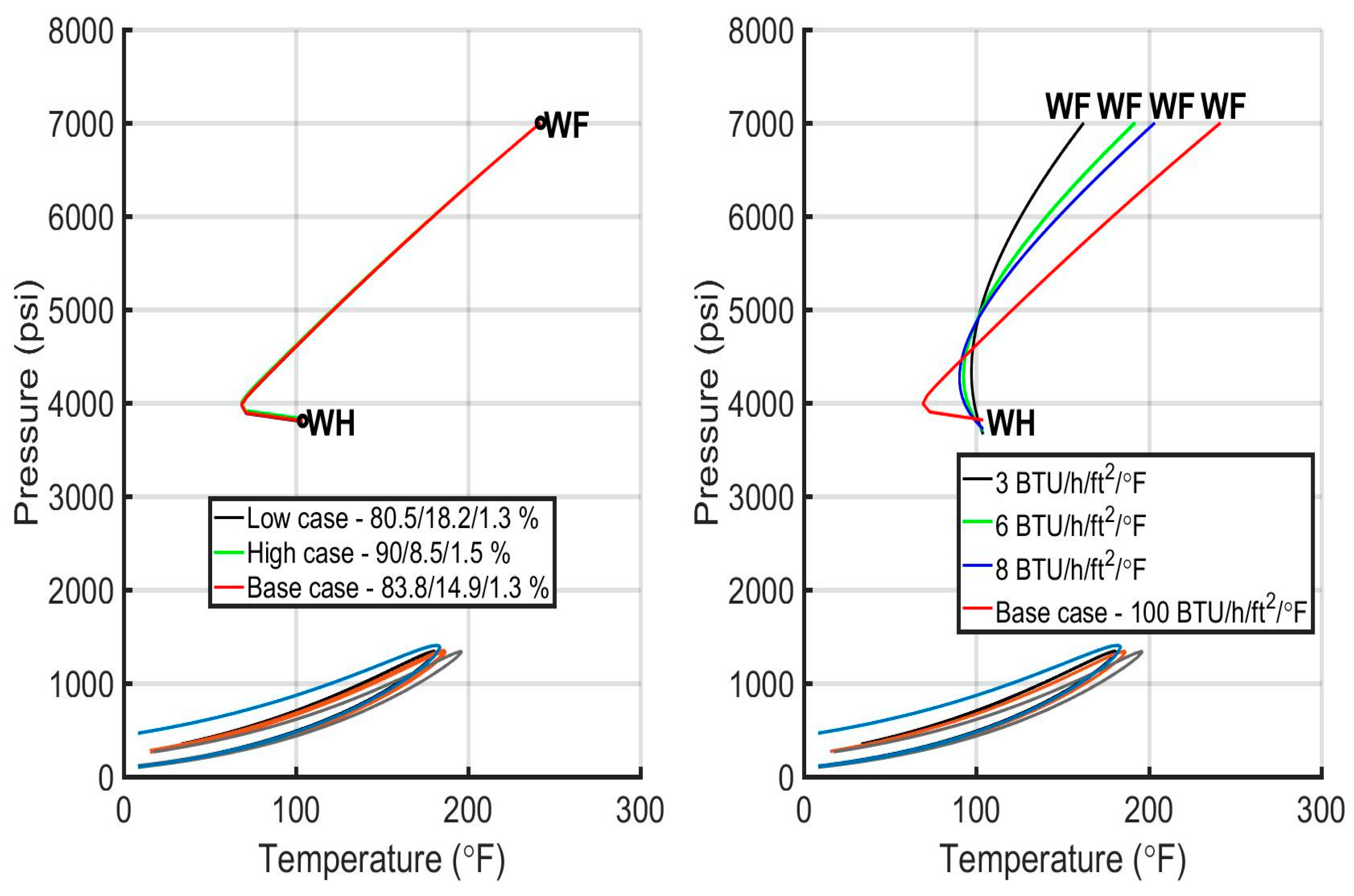
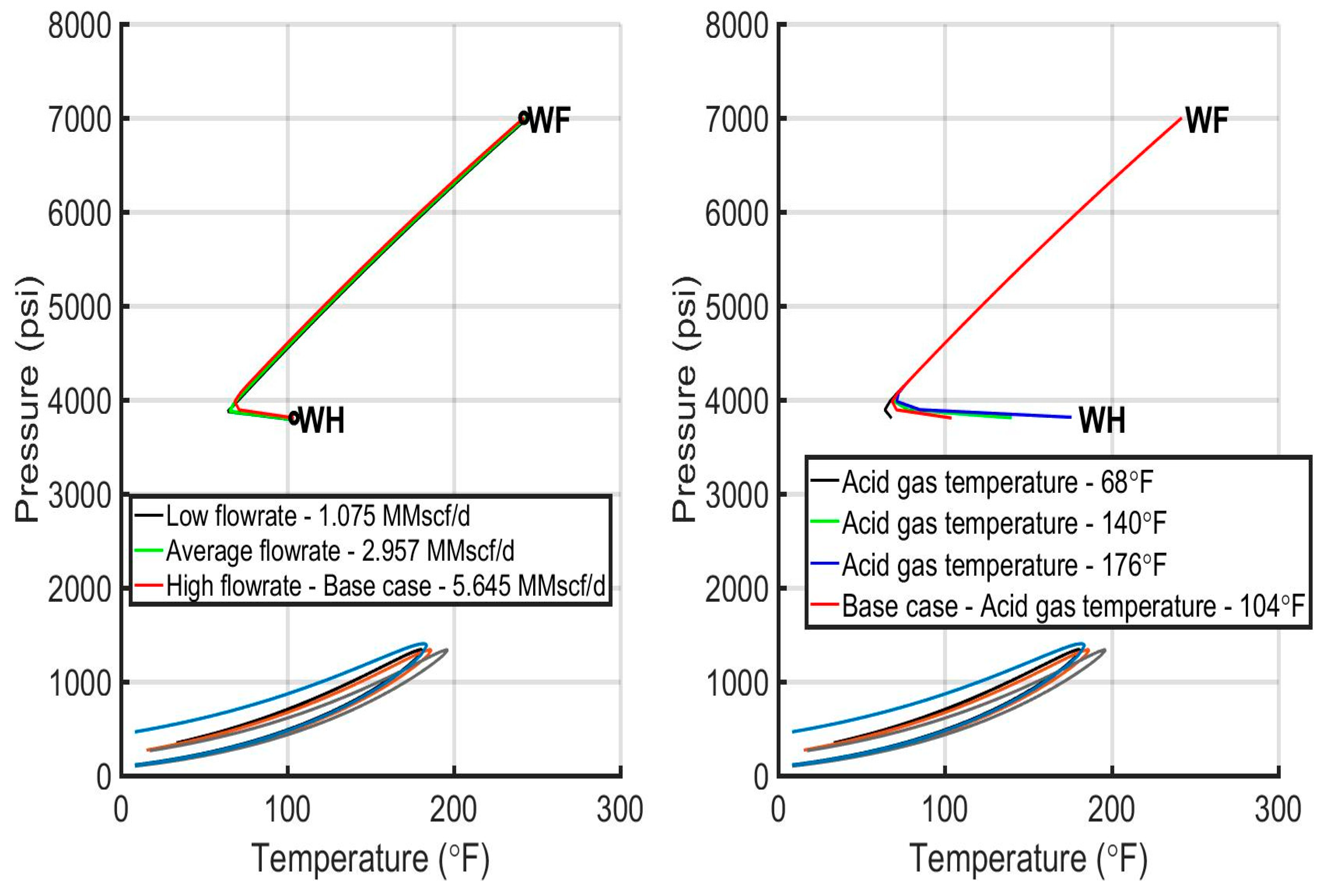
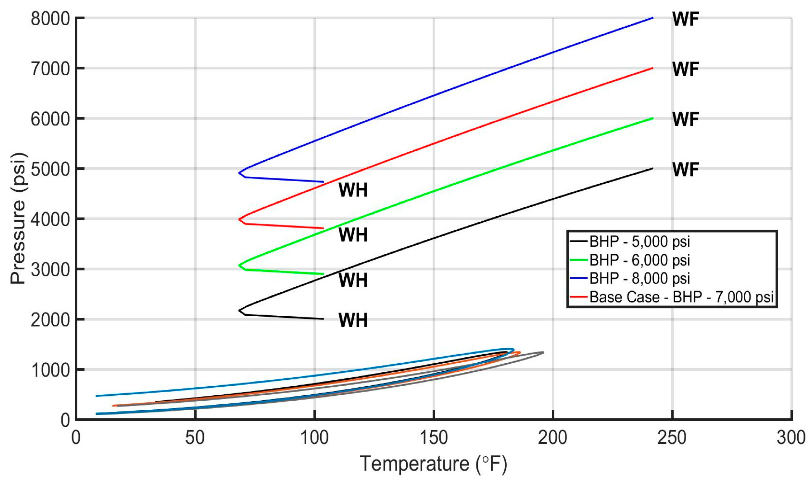
6.3. Evaluation of the Injection Profiles

To run a sensitivity analysis on the parameters of interest (as discussed in Section 3), a base-case scenario is initially set up (

Table 1. Base case scenario.

	Acid Gas Composition (%) H2S/CO2/C1	Heat Transfer Coef. (BTU/h/ft2/°F)	AGI Rate (MMscf/d)	AGI Temperature (°F/°C)	Bottomhole Pressure (psi)
Base case scenario	83.8/14.9/1.5	100	5.645	104/40	7000

), comprising the values that are most likely to occur during the injection process, following the discussion in Section 6.1.

The formation temperature profile was considered to be linear, and since the anticipated AGI rate is expected to be rather slow, thus allowing enough time for the gas to equilibrate thermally with its surroundings, the value of the overall heat transfer coefficient was set at 100 BTU/h/ft²/°F. This value practically corresponds to an instantaneous temperature (40 °C) equilibrium between the injected fluid and the formation. Furthermore, since the design of the surface injection system is not yet finalized, a relatively low acid gas injection temperature was considered to account for the uncertainty of this parameter. Finally, as far as the required bottomhole pressure is concerned, it should be sufficiently higher than the MMP but also capable of covering the flow losses within the formation. According to the MMP estimates (to be discussed in Section 6.4), in combination with experience with regard to the past production of the field, the value that is most likely to occur is in the order of 7000 psi.

The sensitivity analyses were performed using Prosper software [56], and the EoS model built for the acid gas was utilized. The well diameter was set to 73 mm (2 7/8″), all the way to the bottom of the selected injection zone (2900 m), and the surface and bottomhole formation temperature was set to 60 °F and 245 °F, respectively (i.e., the reservoir one). It is worthy of note that the exact survey of the wellbore does not significantly affect the calculations, as the friction pressure loss (which depends on the well’s measured depth) is negligible compared to the gravitational one thanks to the single phase of the flowing acid gas. The injection well P-T profile of the base case scenario is presented in Figure 8.

From the evaluation of the base case injection profile, it is concluded that the injected acid gas is in a liquid or supercritical fluid state from the wellhead (WH) to the bottom of the injection well (WF). This way, the fluid exhibits a safely high value of density throughout its flow path, it produces significant pressure increase due to gravity, and, therefore, it keeps the required pressure at the wellhead low. Furthermore, the profiles lie far away from the phase envelope boundaries, eliminating the risk of two-phase flow in the pipe.

To check whether the P-T conditions along the well may cross the phase envelope due to the acid gas composition variations, four acid gas mixtures (

Table 2. Composition (%) of four acid gas mixtures.

	Low H2S	Average H2S	High H2S	High C1
Composition H2S/CO2/C1 (%)	80.5/18.2/1.3	83.8/14.9/1.3	90/8.5/1.5	83/12/5

) were selected, anticipating the uncertainty in the gas stream composition, and their phase envelopes were plotted (Figure 9). As can be seen, increasing the H₂S content leads to an increase in the T_c and P_c values of the mixture as the phase envelope tends to that of pure H₂S. On the contrary, increasing the CO₂ content reduces T_c and P_c as, this time, the phase envelope tends towards that of pure CO₂. As the methane content increases, the phase envelope begins to expand in pressure and differs more strongly from the “banana shape” of the pure H₂S/CO₂ mixtures. Above the critical point, each fluid exists in the form of a dense phase. Being essentially a binary mixture of components with adjacent characteristics, the two-phase area between the dew and the bubble point has a relatively narrow shape that contrasts with the classic “balloon shape” of conventional hydrocarbon mixtures. Thus, the acid gas may undergo changes from the state of 100% liquid to 100% gas, and vice versa, with only small changes in temperature and/or pressure [9].

Figure 9 shows that the variation of the phase envelopes is quite limited compared to the extent of the acid gas P-T profile. Moreover, the cricondenbar of all phase envelopes lies safely below the base case scenario of the pressure profile. As a result, no border crossing can be safely assumed.

A more detailed sensitivity analysis was carried out to establish whether the crucial and uncertain parameters, shown in Table 1, could significantly affect the fluid behavior in the well (P-T profile) and consequently the $P_{wh}^{Inj}$ during the injection process. A specific range of values was assigned to each parameter separately in order to set up five sensitivity scenarios (

Table 3. Sensitivity analysis cases.

Parameters	Case 1	Case 2	Case 3	Case 4	Case 5
Acid gas composition (%) H2S/CO2/C1	90/8.5/1.5	83.8/14.9/1.3	83.8/14.9/1.3	83.8/14.9/1.3	83.8/14.9/1.3
	80.5/18.2/1.3
Heat transfer coefficient (BTU/h/ft2/F)	100	3	100	100	100
		6
		8
		100
AGI rate (MMscf/d)	5.645	5.645	1.075	5.645	5.645
			2.957
			5.645
AGI temperature (°F/°C)	104/40	104/40	104/40	68/20	104/40
				104/40
				140/60
				176/80
Required bottomhole pressure (psi)	7000	7000	7000	7000	5000
					6000
					7000
					8000

).

For the acid gas composition sensitivity, the composition was selected to vary between those corresponding to the minimum and average acid gas injection rate, as discussed in Section 6.1, whereas the one for the maximum rate case was considered for the base case scenario. Similarly, the acid gas injection rate was allowed to vary between the minimum and average values, as obtained from the production forecast. Due to the lack of data concerning the temperature profile of the well and the effect of heat transfer from the formation to the injected fluid, a wide range of values was chosen that is representative of any possible heat exchange scenario. The value of 3 BTU/h/ft²/°F represents an almost adiabatic temperature profile, while 100 BTU/h/ft²/°F implies a direct temperature equilibrium between the gas and the surrounding formation. Furthermore, to account for any possible acid gas injection temperature values at the wellhead due to the uncertainty in the design of the surface injection facilities, a range from 68 °F to 176 °F (20 °C to 80 °C) was selected to account for the possible heating of the acid gas stream by the compressors or pumps at the surface. Finally, the bottomhole pressure range was set from the fairly low value of 5000 psi to that of 8000 psi (i.e., close to the formation fracture limit) to include all possible scenarios that could have a significant impact on the $P_{wh}^{Inj}$, as well as on the acid gas flow through the wellbore. The results of the sensitivity analysis are as follows:

Case 1 (Figure 10 top left) demonstrates the effect of the increasing acid gas H₂S content on the P-T profile. The resulting profiles for the three sample compositions are almost identical, indicating that acid gas composition variation, to the extent expected to be anticipated in the AGI application studied here, has a negligible effect on the estimated wellhead pressure, $P_{wh}^{Inj}$.

Case 2 (Figure 10 top right) shows the effect of the increasing heat transfer coefficient U on $P_{wh}^{Inj}$. It is observed that U has a minor effect, although temperature itself is severely affected. The difference between the estimated $P_{wh}^{Inj}$ for the min and max values (3 BTU/h/ft²/°F and 100 BTU/h/ft²/°F) is only 4.1%, which is practically negligible, especially when considering the extremity of the two boundary values utilized. Interestingly, although the temperature is greatly affected, which in turn affects fluid density and gravitational pressure gain, the average temperature along the well still varies in a very narrow range, which explains the insensitivity of the gravity term and, eventually, of the estimated $P_{wh}^{Inj}$.

Case 3 (Figure 10 bottom left) investigates the impact of the increasing AGI rate. As expected, the AGI rate has a negligible effect on $P_{wh}^{Inj}$, leading to a variation between the lowest and the highest injection rate in the order of 0.5%. This is explained by the fact that for this specific application, all rates are low enough to allow the temperature of the fluid to quickly match that of the formation and therefore to maintain nearly constant density values. It is reminded that friction pressure loss is insignificant compared to the gravitational one.

Case 4 (Figure 10 bottom right) examines the impact of the acid gas injection temperature. Results show that injection temperature also has a negligible effect on $P_{wh}^{Inj}$, as the pressure value change between the lowest and the highest injection temperature equals 0.26%. This is due to the fact that the injected fluid arrives very quickly at the formation temperature, regardless of its initial value at the injection point.

Case 5 (Figure 11) shows the impact of the increasing bottomhole pressure. Due to its additive effect on $P_{wh}^{Inj}$, this is the only parameter that dramatically affects the required injection pressure. A change in bottomhole pressure from 5000 to 6000 psi causes an increase to a $P_{wh}^{Inj}$ of 36.6%, whereas the corresponding change from 6000 to 7000 psi is 27.2%, and from 7000 to 8000 psi the change is 21.7%.

From Figure 10 and Figure 11, it is verified that for all five sensitivity analyses, the injected acid gas is in a liquid or supercritical fluid state from the wellhead to the bottomhole. This way, the fluid exhibits a safely high value of density throughout its path, produces a significant pressure increase thanks to gravity, and, therefore, keeps the required pressure in the wellhead low. Furthermore, the profiles are significantly distant from the phase envelope boundaries, eliminating the risk of two-phase flow.

6.4. MMP Evaluation

Since no MMP lab measurements are available in the present study, MMP estimation is carried out using established industry MMP correlations by simulating the slim tube test, collecting reliable experimental data from the literature, and running cell-to-cell simulations.

First, the data collected from the literature are presented which correspond to MMP values of the combinations of reservoir fluids and acid gases, similar to those of interest (

Table 4. MMP values retrieved from the literature (AGI with approx. 80% H₂S).

Field	MMP (psi)
KR-G2G (Zama field) (extrapolation)	1900
K oil field (extrapolation)	1960
Field in Kazakhstan (pure H2S)	3000

). Data from the Zama field in Canada [57], the K field in China (the name is classified) [58], and from a field in Kazakhstan (name classified) were retrieved [59].

Compared to the “Prinos” reservoir, the composition of the injected gas and the reservoirs’ temperature differ significantly. In the case of the Zama field, its reservoir temperature is approximately 40 °C lower than that of the Prinos field indicating that the latter’s MMP will be higher, since a temperature increase also causes an MMP value increase. Furthermore, the beneficial intermediate hydrocarbon content of the Zama field is higher than that of Prinos, indicating again a higher MMP for the latter. For those reasons, the results of this approach can only be qualitatively evaluated and used to highlight the positive effect of an increasing H₂S concentration in reducing the required MMP.

Subsequently, the correlations of Emera and Sarma [60] and Shokir [61], representing CO₂–oil systems for pure CO₂ injection streams and CO₂ streams with impurities, were used. These correlations were selected as the most suitable due to their applicability to the prevailing conditions of the “Prinos” field and its fluids. The results obtained are shown in

Table 5. MMP estimations using the correlations of Emera-Sarma and Shokir.

Author	Fluid Context	MMP (psi)
Emera & Sarma	MMP using CO2 stream with impurities	2606
Shokir	MMP using CO2 stream with impurities	2629
Emera & Sarma	MMP using pure CO2	3345

. Keeping in mind that these specific correlations were not developed for H₂S-rich fluids, the predicted MMP values vary from 2606 to 2629 psi. Although those values are slightly high, they still compare well against those obtained from the literature for pure CO₂ (Emera and Sarma, which provide an estimate of 3345) as they only take into account the beneficial effect of H₂S to a limited extent. From this analysis, it is concluded that the exact MMP value should lie below 3000 psi.

For the slim tube simulation, the PVTp software of the IPM suite [62] was used, and a one-dimensional compositional flow numerical model was set up. To account for the uncertain parameters involved in the simulation, a sensitivity analysis (same as in Section 3) was run in terms of (a) the size of the cells (varying number of cells), (b) the Brooks and Corey coefficient values for the relative permeability curves, and (c) the composition of the injected fluid.

For the base case scenario, a numerical model of 10 cells was developed using typical values for the relative permeabilities curves and an acid gas composition of 83, 15, and 2% (CO₂, H₂S, C₁), which is very close to the base case scenario used in Section 6.3. The cell numbers were subsequently increased from the base case scenario value to 40 cells, while keeping the slim tube length constant; the Brooks and Corey coefficient value was increased from λ = 0.5 (broad pore size distribution) to λ = 3.7 (narrow pore size distribution) followed by an increase in H₂S and CH₄ content in the injection fluid. The simulation scenarios, along with the corresponding MMP predicted values, are presented in

Table 6. Results of the slim tube test.

Parameter	Scenarios	MMP (psi)
-	Base case scenario (10 cells)	2400
Cell Size	Increased cells number (40 cells)	2400
Rel. perm. curves	Brooks and Corey (λ = 0.5)	2400
	Brooks and Corey (λ = 3.7)	2400
Injected gas composition	78% H2S—20% CO2—2% CH4	2500
	83% H2S—15% CO2—2% CH4	2400
	88% H2S—10% CO2—2% CH4	2250
	70% H2S—20% CO2—10% CH4	3300

.

As can be seen from the results, quadrupling the number of cells in the simulation model while keeping the other parameters constant shows that numerical dispersion, which is an inherent problem in reservoir simulation, does not affect the MMP estimate, as the latter is a volumetric property. Similar reasoning explains why changes in Brooks and Corey’s coefficient values also do not affect the MMP value. On the other hand, the increase of H₂S and CH₄ content in the injection fluid were the only parameters that affected the MMP value. More specifically, the estimated MMP decreased with increasing H₂S content, while a steep increase was observed with the CH₄ mixture enrichment, with both observations being in full accordance with the engineers’ experience [63]. Clearly, methane needs to be removed to the best possible level so as to avoid an undesired MMP increase. The results demonstrate that the expected MMP value is in the order of 2400 psi or lower.

For the cell-to-cell simulation, the four acid gas compositions utilized in the slim tube test were repeated in this simulation. Each gas was mixed with the reservoir oil at increasing ratios, in steps of 5%. When two-phase mixtures were obtained, the equilibrium phases were further mixed to the alternate phase (acid gas or reservoir oil) at the same increasing step until miscibility or a dead end was encountered. The condensing gas drive mechanisms investigation did not lead to miscibility at all pressures attempted. However, miscibility was achieved for all four trial gas compositions by means of the vaporizing drive mechanism. The estimated MMP values are in full accordance with the findings of the tests above verifying an MMP value slightly above 2200 psi (see

Table 7. Results of the cell-to-cell simulation.

Injected Gas Composition (%): H2S/CO2/C1	MMP (psi)
78/20/2	2238
83/15/2	2225
88/10/2	2200
70/20/10	2363

). As expected, increasing methane content (from 2 to 10 mol%) led to an increase of the MMP value by approximately 150 psi.

By combining the results from all four approaches, an MMP estimate between 2200 to 2400 psi was finally obtained for the Prinos reservoir.

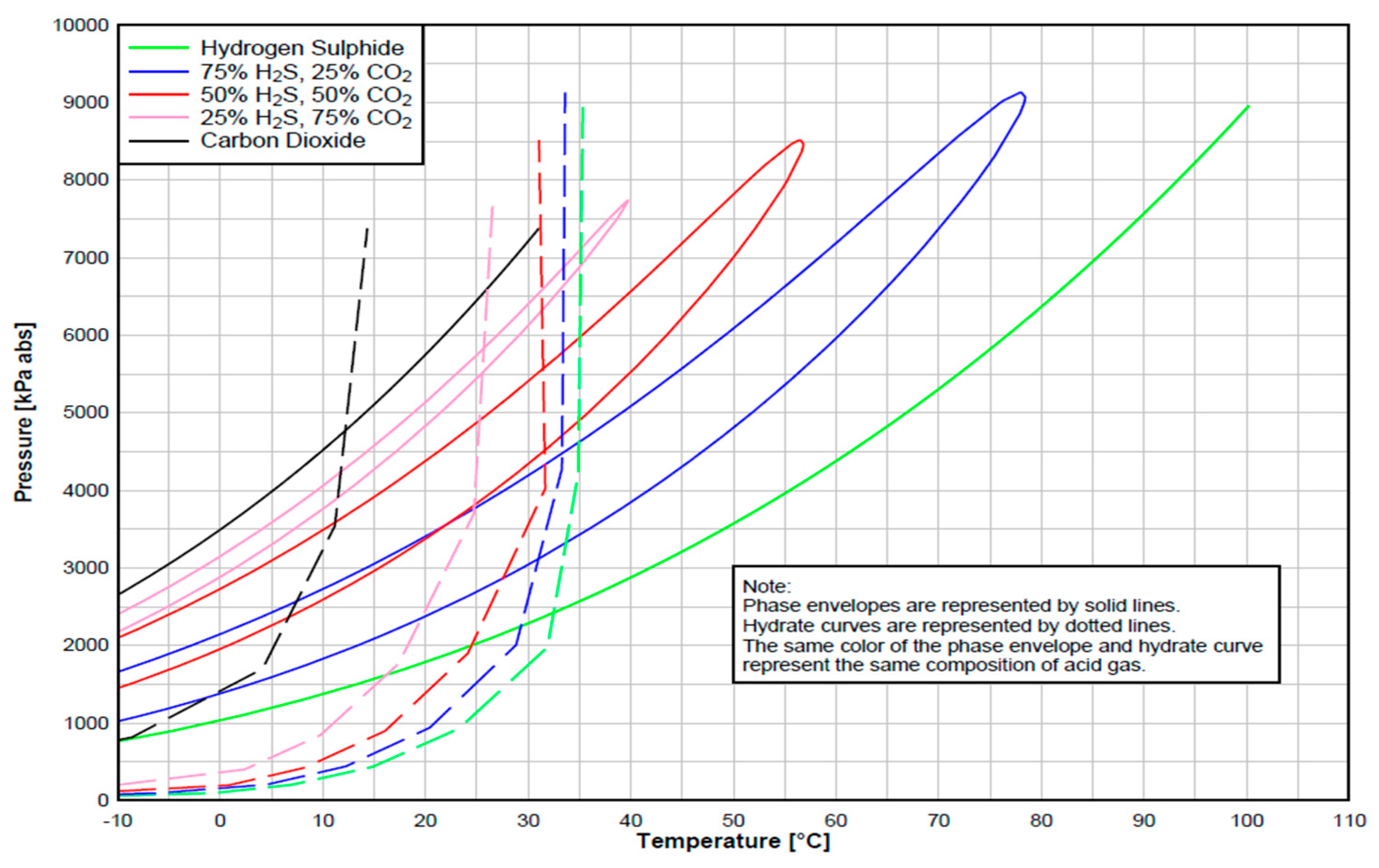
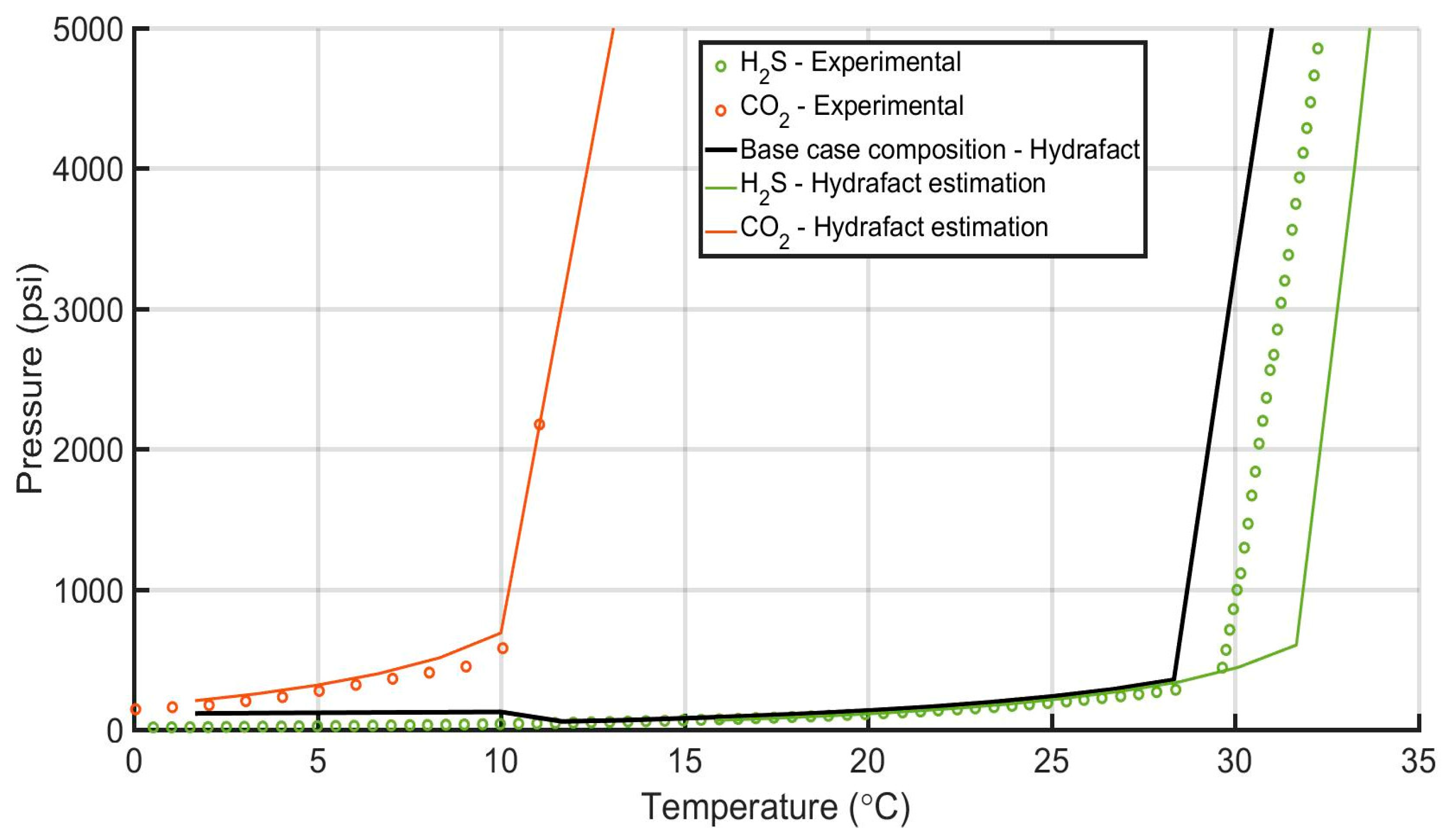
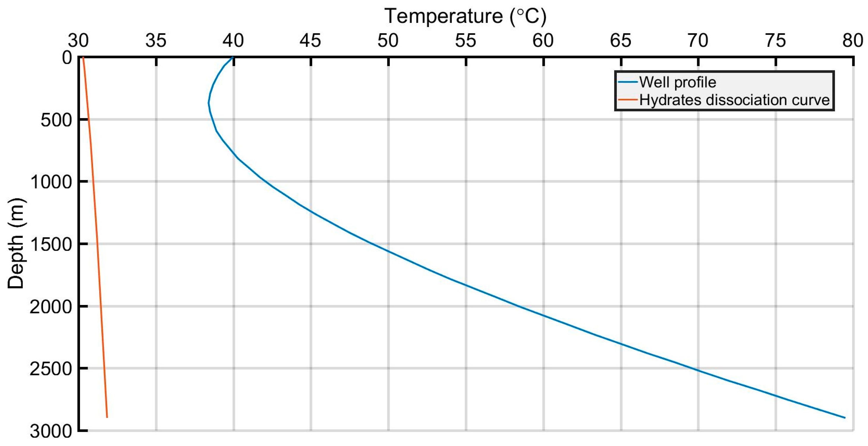
6.5. Hydrate Formation Conditions

To assess flow assurance issues that might occur during AGI in the “Prinos” field, the hydrate formation conditions were evaluated using the solids thermodynamic model implemented in the HydraFLASH software (v. 2.2). For a given H₂O/HC/inhibitor mixture, HydraFLASH uses the multiphase equilibrium algorithm of Michelsen [64], the Van der Waals and Platteeuw theory, and the CPA EoS [65] to predict the hydrate dissociation curve for the acid gas mixture of interest.

Before using the software, it is necessary to evaluate its accuracy, as its parameters (such as component properties, Langmuir coefficients and Kihara potentials) have already been tuned by the developers [66]. For this task, experimental data of hydrate formation conditions collected from the literature is used to evaluate the selected model performance, although the experimental data available for acid gas mixtures is limited.

First, the experimental hydrate dissociation curves of the two pure components, that of H₂S [67,68] and of CO₂ [69], were retrieved and plotted in dashed lines a P-T diagram (Figure 12) to qualitatively study hydrate formation, in combination with various comments and observations appearing in the literature. This data practically delineates the hydrate formation region within which all H₂S-CO₂ acid gas hydrate mixture curves should be located. Furthermore, in order to demonstrate the software’s capability of predicting the hydrate formation curve for the base case composition, an error analysis was conducted in order to check the software-derived pure CO₂ and H₂S hydrate formation curves against their corresponding available experimental data.

The observations of Wu & Carroll [70] provide useful insight into the calculated hydrate formation curves of three characteristic acid gas mixtures of varying H₂S and CO₂ content, namely 75%/25%, 50%/50% and 25%/75%. These dashed line curves, although not experimental, are the product of AQUAlibrium 3.1 software [71], a product dedicated to acid gas and water equilibria calculations. Clearly, the highest and the lowest formation temperatures correspond to pure H₂S and pure CO₂ respectively. The three test acid gas mixtures lie perfectly between these two curves, with decreasing maximum formation temperature as H₂S decreases.

Figure 13 illustrates the error analysis and the computed (by means of HydraFLASH) formation curve (green line) for the base case scenario (83.8/14.9/1.3% H₂S/CO₂/C₁ %), verifying the following:

(1) For the case of H₂S, the maximum deviation of experimental hydrate formation temperature data is approximately 1.5 °C and only at pressures above 500 psi, whereas for the case of CO₂, the estimates are excellent over the entire pressure range. As a result, the software estimate for the base case composition is quite representative of the true hydrate formation conditions.

(2) The observations of Wu & Carroll [70] are confirmed in the sense that an increased hydrate formation temperature is obtained for the H₂S-rich acid gas mixture available in this work. In fact, if the H₂S content of the mixture exceeds about 30%, the hydrate formation temperature lies very close to that of pure H₂S.

(3) A temperature close to 30 °C seems to be the critical limit below which hydrate formation is expected for the acid gas mixture considered in the “Prinos” AGI project. Therefore, hydrates cannot form within the acid gas injection very well, since the temperatures developed within are always very high and are safely above the highest hydrate formation temperature of approximately 30 °C. This is also demonstrated in Figure 14, which shows the hydrate temperature profile together with the wellbore one along the depth. No line crossing takes place throughout the entire temperature range and, thus, the formation of hydrates within the acid gas injection well is not possible. Note that the low-pressure part of the hydrates curve is not shown, as the well is already pressurized (3500–7000 psi).

7. Conclusions

A workflow was proposed that aimed at the development of all necessary computational tools for predicting the thermodynamic properties of the fluids involved in the design of an AGI project. The EoS model proposed for the acid gas and the reservoir fluid was based on the PR-78 EoS, since it performs accurately and is supported by all commercial simulation software. Subsequently, the developed EoS was used to investigate various aspects of the AGI where thermodynamics are the major player. First, an investigation of the prevailing conditions (P-T) along the injection well (injection profiles) was suggested to ensure a single-phase state flow of the acid gas inside the well and the adequate arrival bottomhole pressure to achieve full miscibility. Subsequently, a set of tools was provided to estimate the MMP using analogs, correlations applicable to H₂S-rich systems, and computational simulations. Finally, it was recommended that the flow resistance be examined, as it may lead to severe issues such as pipeline blockage during the AGI project implementation.

The workflow was implemented in the “Prinos” field in Northern Greece, and the detailed results obtained verified the validity of the proposed workflow. The developed EoS model provided all information required in the bottom-up design approach, which departs from the reservoir and arrives at the injection wellhead, thus providing all necessary information to the surface equipment facilities design step that will follow.

References

1. Siddiqui, M.I.; Baber, S.; Saleem, W.A.; Jafri, M.O.; Hafeez, Q. Industry practices of sour gas management by reinjection: Benefits, methodologies, economic evaluation and case studies. In Proceedings of the SPE/PAPG Annual Technical Conference, Islamabad, Pakistan, 26–27 November 2013; p. SPE-169645-MS. [Google Scholar]
2. Kokal, S.L.; Al-Utaibi, A. Sulfur Disposal by Acid Gas Injection: A Road Map and A Feasibility Study. In Proceedings of the SPE Middle East Oil and Gas Show and Conference, Al Manama, Bahrain, 12–15 March 2005; p. SPE-93387-MS. [Google Scholar]
3. Burgers, W.F.J.; Northrop, P.S.; Kheshgi, H.S.; Valencia, J.A. Worldwide development potential for sour gas. Energy Procedia 2011, 4, 2178–2184. [Google Scholar] [CrossRef] [Green Version]
4. Maddocks, J. Capacity Control Considerations for Acid Gas Injection Systems; Gas Liquids Engineering Ltd.: Calgary, AB, Canada, 2015. [Google Scholar]
5. Bachu, S.; Gunter, W.D. Overview of acid-gas injection operations in Western Canada. In Proceedings of the 7th International Conference on Greenhouse Gas Control Technologies, Vancouver, BC, Canada, 5 September 2004. [Google Scholar]
6. Mokhatab, S.; Poe, W.A.; Mak, J.W. Handbook of Natural Gas Transmission and Processing, 4th ed.; Gulf Professional Publishing: Cambridge, MA, USA, 2019; ISBN 978-0-12-815817-3. [Google Scholar]
7. Carroll, J.J. Acid gas injection: Past, present, and future. In Proceedings of the International Acid Gas Injection Symposium, Calgary, AB, Canada, 5–6 October 2009. [Google Scholar]
8. Zhou, J.; Chen, J.-Y.; Gao, P.-C.; Tang, H.-J. Wellbore flow model of acid gas reinjection. Nat. Gas Ind. 2005, 25, 76–78. [Google Scholar]
9. Mireault, R.A.; Stocker, R.; Dunn, D.W.; Pooladi-Darvish, M. Wellbore dynamics of acid gas injection well operation. In Proceedings of the Canadian Unconventional Resources and International Petroleum Conference, Calgary, AB, Canada, 19–21 October 2010; p. SPE-135455-MS. [Google Scholar]
10. Carroll, J.J. Acid Gas Injection—The Next Generation; Gas Liquids Engineering Ltd.: Calgary, AB, Canada, 2009. [Google Scholar]
11. International Energy Agency Greenhouse Gas R&D Program. Acid Gas Injection: A Study of Existing Operations, Phase I: Final Report, PH4/18; IEAG: Cheltenham, UK, 2003. [Google Scholar]
12. Bachu, S.; Gunter, W. Acid-gas injection in the Alberta basin, Canada: A CO2-storage experience. Geol. Soc. 2004, 233, 225–234. [Google Scholar] [CrossRef]
13. Malik, Z.; Charfeddine, M.; Moore, S.; Francia, L.; Denby, P. The Supergiant Kashagan Field: Making a Sweet Development Out of Sour Crude. In Proceedings of the International Petroleum Technology Conference, Doha, Qatar, 21–23 November 2005; p. IPTC-10636-MS. [Google Scholar]
14. Abou-Sayed, A.S.; Summers, C.; Zaki, K.S. An Assessment of Engineering Economical and Environmental Drivers of Sour Gas Management by Injection. In Proceedings of the SPE International Improved Oil Recovery Conference in Asia Pacific, Kuala Lumpur, Malaysia, 5–6 December 2005; p. SPE-97628-MS. [Google Scholar]
15. Urazgaliyeva, G.; King, G.R.; Darmentaev, S.; Tursinbayeva, D.; Dunger, D.; Howery, R.; Zalan, T.; Lindsell, K.; Iskakov, E.; Turymova, A.; et al. Tengiz Sour Gas Injection Project: An Update. In Proceedings of the SPE Annual Caspian Technical Conference and Exhibition, Astana, Kazakhstan, 12–14 November 2014; p. SPE-172284-MS. [Google Scholar]
16. Miwa, M.; Shiozawa, Y.; Saito, Y.; Tarmoom, I.O. Sour Gas Injection Project. In Proceedings of the Abu Dhabi International Petroleum Exhibition and Conference, Abu Dhabi, United Arab Emirates, 13–16 October 2002; p. SPE-78547-MS. [Google Scholar]
17. Haynes, B.; Kaura, N.C.; Faulkner, A. Life Cycle of a depletion drive and sour gas injection development: Birba A4C Reservoir, South Oman. In Proceedings of the International Petroleum Technology Conference, Kuala Lumpur, Malaysia, 3–5 December 2008; p. IPTC-12175-MS. [Google Scholar]
18. Battistelli, A.; Ceragioli, P.; Marcolini, M. Injection of Acid Gas Mixtures in Sour Oil Reservoirs: Analysis of Near-Wellbore Processes with Coupled Modelling of Well and Reservoir Flow. Transp. Porous Media 2011, 90, 233–251. [Google Scholar] [CrossRef]
19. Adewumi, M. Phase Relations in Reservoir Engineering; Pennsylvania State University: State College, PA, USA, 2022. [Google Scholar]
20. Chapoy, A.; Coquelet, C.; Liu, H.; Valtz, A.; Tohidi, B. Vapor-liquid equilibrium data for the hydrogen sulfide (H2S) + carbon dioxide (CO2) system at temperatures from 258 to 313 K. Fluid Phase Equilibria 2013, 356, 223–228. [Google Scholar] [CrossRef]
21. Stamataki, S.; Magoulas, K. Predictions of Phase Equilibria and Volumetric Behavior of Fluids with High Concentration of Hydrogen Sulfide. Oil Gas Sci. Technol. 2000, 55, 511–522. [Google Scholar] [CrossRef] [Green Version]
22. Ahmed, T. Reservoir Engineering Handbook, 4th ed.; Elsevier: Amsterdam, The Netherlands, 2010; ISBN 9780080966670. [Google Scholar]
23. Tsivintzelis, I.; Kontogeorgis, G.M.; Michelsen, M.L.; Stenby, E.H. Modeling phase equilibria for acid gas mixtures using the CPA equation of state. I. Mixtures with H2S. AIChE J. 2010, 56, 2965–2982. [Google Scholar] [CrossRef]
24. Computer Modelling Group Ltd. WinProp User Guide. Phase Property Program; Version 2010; Computer Modelling Group Ltd.: Calgary, AB, Canada, 2010. [Google Scholar]
25. Gaganis, V.; Kourlianski, E.; Varotsis, N. An accurate method to generate composite PVT data for Black Oil Simulation. J. Pet. Sci. Eng. 2007, 157, 1–13. [Google Scholar] [CrossRef]
26. Pedersen, K.S.; Blilie, A.L.; Meisingset, K.K. PVT Calculations on petroleum reservoir fluid using measured and estimated composition data for the plus fraction. Ind. Eng. Chem. Res. 1992, 31, 1378–1384. [Google Scholar] [CrossRef]
27. Whitson, C.H. Characterizing hydrocarbon plus fractions. SPE J. 1983, 23, 683–694. [Google Scholar] [CrossRef]
28. Chueh, P.L.; Prausnitz, J.M. Vapor-liquid equilibria at high pressures: Calculation of partial molar volumes in nonpolar liquid mixtures. AIChE J. 1967, 13, 1099–1107. [Google Scholar] [CrossRef]
29. Kordas, A.; Tsoutsouras, K.; Stamataki, S.; Tassios, D. A generalized correlation for the interaction coefficients of CO2—Hydrocarbon binary mixtures. Fluid Phase Equilibria 1994, 93, 141–166. [Google Scholar] [CrossRef]
30. Jhaveri, B.S.; Youngren, G.K. Three parameters modification of the Peng-Robinson Equation of State to improve volume predictions. SPE Reserv. Eng. 1988, 3, 1033–1140. [Google Scholar] [CrossRef]
31. Anastasiadou, V.; Samnioti, A.; Kanakaki, R.; Gaganis, V. Acid gas re-injection system design using machine learning. Clean Technol. 2022, 4, 1001–1019. [Google Scholar] [CrossRef]
32. Tureyen, O.I.; Karaalioglu, H.; Satman, A. Effect of the Wellbore Conditions on the Performance of Underground Gas-Storage Reservoirs. In Proceedings of the SPE/CERI Gas Technology Symposium, Calgary, AB, Canada, 3–5 April 2000; p. SPE-59737-MS. [Google Scholar]
33. Rigzone. How Does Gas Injection Work? Available online: https://www.rigzone.com/training/insight?insight_id=345&c_id= (accessed on 15 September 2022).
34. Green, D.W.; Willhite, G.P. Enhanced Oil Recovery, 2nd ed.; Society of Petroleum Engineers: Richardson, TX, USA, 2018; ISBN 978-1-61399-494-8. [Google Scholar]
35. Li, Q.; Wu, J. Factors affecting the lower limit of the safe mud weight window for drilling operation in hydrate-bearing sediments in the Northern South China Sea. Geomech. Geophys. Geo-Energy Geo-Resour. 2022, 8, 82. [Google Scholar] [CrossRef]
36. Wei, W.N.; Li, B.; Gan, Q.; Li, Y.L. Research progress of natural gas hydrate exploitation with CO2 replacement: A review. Fuel 2022, 312, 122873. [Google Scholar] [CrossRef]
37. Li, Q.; Wang, F.; Forson, K.; Zhang, J.; Zhang, C.; Chen, J.; Xu, N.; Wang, Y. Affecting analysis of the rheological characteristic and reservoir damage of CO2 fracturing fluid in low permeability shale reservoir. Environ. Sci. Pollut. Res. 2022, 29, 7815–37826. [Google Scholar] [CrossRef]
38. Kodera, M.; Matsueda, T.; Belosludov, R.V.; Zhdanov, R.K.; Belosludov, V.R.; Takeya, S.; Alavi, S.; Ohmura, R. Physical properties and characterization of the binary clathrate hydrate with methane + 1,1,1,3,3-Pentafluoropropane (HFC-245fa) + Water. J. Phys. Chem. C 2020, 124, 20736–20745. [Google Scholar] [CrossRef]
39. Ripmeester, J.A.; Tse, J.S.; Ratcliffe, C.I.; Powell, B.M. A new clathrate hydrate structure. Nature 1987, 325, 135–136. [Google Scholar] [CrossRef]
40. Koh, C.A.; Sloan Jr, E.D. Clathrate Hydrates of Natural Gases; CRC Press: Boca Raton, FL, USA, 2007; ISBN 9780849390784. [Google Scholar]
41. Zatsepina, O.Y.; Buffett, B.A. Thermodynamic conditions for the stability of gas hydrate in the seafloor. J. Geophys. Res. Solid Earth 1998, 103, 24127. [Google Scholar] [CrossRef]
42. Davidson, D.W.; Garg, S.K.; Gough, S.R.; Handa, Y.P.; Ratcliffe, C.I.; Ripmeester, J.A.; Tse, J.S.; Lawson, W.F. Laboratory analysis of a naturally occurring gas hydrate from sediment of the Gulf of Mexico. Geochim. Cosmochim. Acta 1986, 50, 619–623. [Google Scholar] [CrossRef]
43. Bharathi, A.; Nashed, O.; Lal, B.; Foo, K.S. Experimental and modelling studies on enhancing the thermodynamic hydrate inhibition performance of monoethylene glycol via synergistic green material. Sci. Rep. 2021, 11, 2396. [Google Scholar] [CrossRef] [PubMed]
44. Elgibaly, A.A.; Elkamel, A.M. A new correlation for predicting hydrate formation conditions for various gas mixtures and inhibitors. Fluid Phase Equilibria 1998, 152, 23–42. [Google Scholar] [CrossRef]
45. Van der Waals, J.H.; Platteeuw, J.C. Clathrate solutions. In Advances in Chemical Physics; Wiley: Hoboken, NJ, USA, 1959; ISBN 9780470143483. [Google Scholar]
46. Hydrafact PVT and Flow Assurance. HydraFLASHTM PVT and Flow Assurance Prediction Software. Available online: https://www.hydrafact.com/products/hydraflash/ (accessed on 1 November 2022).
47. KBC Global. A Yokogawa Company. Gas Hydrates Modeling with CPA. Available online: https://www.kbc.global/resources/whitepapers/gas-hydrates-modeling-with-cpa/ (accessed on 1 November 2022).
48. Offshore Technology. Prinos Offshore Development Project, North Aegean Sea, Gulf of Kavala. Available online: https://www.offshore-technology.com/projects/prinos-offshore-development-project-north-aegean-sea-gulf-of-kavala/ (accessed on 1 October 2022).
49. Proedrou, P.; Papaconstantinou, C.M. Prinos basin—A model for oil exploration. Bull. Geol. Soc. Greece 2004, 36, 327–333. [Google Scholar] [CrossRef]
50. Kiomourtzi, P.; Pasadakis, N.; Zelilidis, A. Source Rock and Depositional Environment Study of Three Hydrocarbon Fields in Prinos—Kavala Basin (North Aegean). Open Pet. Eng. J. 2008, 1, 16–29. [Google Scholar] [CrossRef] [Green Version]
51. Bierlein, J.A.; Kay, W.B. Phase Equilibrium Properties of System Carbon Dioxide Hydrogen Sulfide. Ind. Eng. Chem. 1953, 45, 618–624. [Google Scholar] [CrossRef]
52. Kellerman, S.J.; Stouffer, C.E.; Eubank, P.T.; Holste, J.C.; Hall, K.R. Thermodynamic Properties of CO2 + H2S Mixtures: Project 842; Gas Processors Assoc.: Tulsa, OK, USA, 1995; ISBN 1567000495. [Google Scholar]
53. Bennion, D.B.; Thomas, F.B.; Schulmeister, B.E.; Imer, D.; Shtepani, E.; Becker, L. The Phase Behavior of Acid Disposal Gases and the Potential Adverse Impact on Injection or Disposal Operations. J. Can. Pet. Technol. 2004, 43, PETSOC-04-05-01. [Google Scholar] [CrossRef]
54. Goodwin, R.D. Hydrogen Sulfide Provisional Thermophysical Properties From 188 to 700 K at Pressure to 75 MPa; National Bureau of Standards, Chemical Engineering Science Division, U.S. Department of Commerce: Boulder, CO, USA, 1983. [Google Scholar]
55. Commodore, J.A.; Deering, C.E.; Bernard, F.; Marriott, R.A. High-pressure densities and excess molar volumes for the binary mixture of carbon dioxide and hydrogen sulfide at T = 343 to 397 K. J. Chem. Eng. Data 2021, 66, 4236–4247. [Google Scholar] [CrossRef]
56. Petroleum Experts Ltd. Prosper User Manual; Version 12; Petroleum Experts Ltd.: Edinburgh, UK, 2013. [Google Scholar]
57. Sayegh, S.; Huang, S.; Zhang, Y.P.; Lavoie, R. Effect of H2S and pressure depletion on the CO2 MMP of Zama oils. J. Can. Pet. Technol. 2007, 46, PETSOC-07-08-03. [Google Scholar] [CrossRef]
58. Lv, S.; Liao, X.; Chen, H.; Chen, Z.; Lv, X.; Zhou, X. Predicting the Effects of Acid Gas on Enhanced Oil Recovery in Hydrocarbon Gas Injection. In Proceedings of the SPE Western Regional Meeting, Anchorage, AK, USA, 23–26 May 2016; p. SPE-180434-MS. [Google Scholar]
59. He, C.; Mu, L.; Xu, A.; Zhao, L.; He, J.; Zhang, A.; Shan, F.; Luo, E. Phase behavior and miscible mechanism in the displacement of crude oil with associated sour gas. Oil Gas Sci. Technol. 2019, 74, 54. [Google Scholar] [CrossRef] [Green Version]
60. Emera, M.; Sarma, H. A reliable correlation to predict the change in minimum miscibility pressure when CO2 is diluted with other gases. SPE Reserv. Eval. Eng. 2006, 9, 366–373. [Google Scholar] [CrossRef]
61. Shokir, E.M.E.M. Precise model for estimating CO2-oil minimum miscibility pressure. Pet. Chem 2007, 47, 368–376. [Google Scholar] [CrossRef]
62. Petroleum Experts Ltd. PVTP User Manual; Version 10; Petroleum Experts Ltd.: Edinburgh, UK, 2016. [Google Scholar]
63. Jin, L.; Pekot, L.G.; Hawthorne, S.B.; Gobran, B.; Greeves, A.; Bosshart, N.W.; Jiang, T.; Hamling, J.A.; Gorecki, C.D. Impact of CO2 impurity on MMP and oil recovery performance of the Bell Creek oil field. Energy Procedia 2017, 114, 6997–7008. [Google Scholar] [CrossRef]
64. Michelsen, M.L. Multiphase isenthalpic and isentropic flash algorithms. Fluid Phase Equilibria 1987, 33, 13–27. [Google Scholar] [CrossRef]
65. Palma, A.M.; Queimada, A.J.; Coutinho, J. Modelling Hydrate Dissociation Curves in the presence of hydrate inhibitors with a modified CPA EoS. Ind. Eng. Chem. Res. 2019, 58, 19239–19250. [Google Scholar] [CrossRef]
66. Ismail, I.; Gaganis, V.; Marinakis, D.; Mousavi, R.; Tohidi, B. Accuracy of different thermodynamic software packages in predicting hydrate dissociation conditions. Chem. Thermodyn. Therm. Anal. 2022, 9, 100103. [Google Scholar] [CrossRef]
67. Sun, J.; Xin, Y.; Chou, I.-M.; Sun, R.; Jiang, L. Hydrate stability in the H2S-H2O system—Visual observations and measurements in a high-pressure optical cell and thermodynamic models. J. Chem. Eng. Data 2020, 65, 3884–3892. [Google Scholar] [CrossRef]
68. Selleck, F.T.; Carmichael, L.T.; Sage, B.H. Phase Behavior in the Hydrogen Sulfide-Water System. Ind. Eng. Chem. 1952, 44, 2219–2226. [Google Scholar] [CrossRef]
69. Wikipedia. The Free Encyclopedia. Carbon Dioxide Clathrate. Available online: https://en.wikipedia.org/wiki/Carbon_dioxide_clathrate (accessed on 1 December 2022).
70. Wu, Y.; Carroll, J.J. The research on experiments and theories about hydrates in high-sulfur gas reservoirs. In Acid Gas Injection and Related Technologies; Wiley: Hoboken, NJ, USA, 2011; ISBN 978-1-118-09426-6. [Google Scholar]
71. Gas Liquids Engineering. AQUAlibrium Software. Available online: https://www.gasliquids.com/software-library/ (accessed on 15 September 2022).
72. Grynia, E.W.; Carroll, J.J.; Griffin, P.J. Dehydration of acid gas prior to injection. In Proceedings of the 2nd Annual Gas Processing Symposium, Doha, Qatar, 10–14 January 2010; pp. 177–185. [Google Scholar]
Figure 1. Acid gas treatment and reinjection process.
Energies 16 02392 g001
Figure 2. Proposed workflow for reservoir and wellbore appraisal during AGI for EOR.
Energies 16 02392 g002
Figure 3. Reverse calculation procedure for the estimation of the required wellhead pressure [33].
Energies 16 02392 g003
Figure 4. Prinos–Kavala Offshore basin [50].
Energies 16 02392 g004
Figure 5. Experimental and estimated phase envelopes of pure H2S, CO2, and acid gas mixtures.
Energies 16 02392 g005
Figure 6. Experimental and estimated densities of the multicomponent mixture (H2S-CO2-CH4).
Energies 16 02392 g006
Figure 7. Estimates of the volumetric property predictions against CCE and DLE experimental data.
Energies 16 02392 g007
Figure 8. Injection well P-T profile of the base case scenario.
Energies 16 02392 g008
Figure 9. Phase envelopes for the four acid gas mixtures.
Energies 16 02392 g009
Figure 10. Parameters with a negligible or very small effect on wellhead pressure.
Energies 16 02392 g010aEnergies 16 02392 g010b
Figure 11. Parameters with significant effect on wellhead pressure.
Energies 16 02392 g011
Figure 12. Hydrate formation curves [72].
Energies 16 02392 g012
Figure 13. Prediction of the hydrate dissociation curve with the HydraFLASH software.
Energies 16 02392 g013
Figure 14. Comparison of the predicted hydrate formation dissociation curve to the temperature profile along the wellbore.
Energies 16 02392 g014