Abstract
The distribution network reconfiguration problem (DNRP) refers to the challenge of searching for a given power distribution network configuration with better operating conditions, such as minimized energy losses and improved voltage levels. To accomplish that, this paper revisits the branch exchange heuristics and presents a method in which it is coupled with other techniques such as evolutionary metaheuristics and cluster analysis. The methodology is applied to four benchmark networks, the 33-, 70-, 84-, and 136-bus networks, and the results are compared with those available in the literature, using the criteria of the number of power flow executions. The methodology minimized the four systems starting from the initial configuration of the network. The main contributions of this work are the use of clustering techniques to reduce the search space of the DNRP; the consideration of voltage regulation banks and voltage-dependent loads in the feeder, requiring the addition of a constraint to the mono-objective model to guarantee the transferred load will be supplied at the best voltage magnitude level, and the application of the methodology in real distribution networks to solve a set of 81 real DNRPs from CEMIG-D (the distribution branch of the Energy Company of Minas Gerais). Four out of those are presented as case studies to demonstrate the applicability of the approach, which efficiently found configurations with lower power and energy losses with few PF runs.
1. Introduction
The distribution network reconfiguration problem (DNRP) is often employed to improve a distribution network’s operational conditions, which are evaluated through indicators such as power loss summation and voltage deviation [1]. The DNRP is solved by changing the statuses of switching devices, such as outdoor switches and reclosers, to obtain a new network configuration under better operational conditions. This new configuration must also comply with the usual system constraints in the DNRP model, including voltage limits, line capacities, and network radiality. The DNRP is highly combinatorial for the exponential growth of the number of possible configurations as the number of tie switches increases. As stated in [2], the development of a very fast technique to estimate the power losses of the proposed configurations is a challenge for the DNRP. Furthermore, the DNRP model is nonlinear, mixed-integer, and non-differentiable. These characteristics point towards the use of metaheuristics as the most suitable class of techniques for the solution. In this sense, it is worth mentioning that the number of published works tackling DNRP through metaheuristics is higher than those based on heuristics or mathematical optimization approaches [1].
Generally, the technical literature has shown the mono-objective formulation for optimization as the recurrent alternative since the main objective is the minimization of technical losses. Furthermore, the mono-objective form with power loss minimization remains the single most important objective for the majority of the published works [2,3,4] and is the adopted formulation for the present work. However, the multi-objective form is usually preferred to deal with the network restoration problem. In this problem, the objectives usually include the network reliability indexes [5], the number of switch maneuvers to the service restoration [6], and the number of disconnected clients [7].
Currently, the distribution networks have incorporated more possibilities for reconfiguration due to the increasing penetration of distributed energy resources (DER), which demands more frequent reconfigurations to minimize power losses [8], and the increase in intelligent electronic devices (IED), such as outdoor vacuum reclosers, which allow remote operations. In the last decade, the DNR has advanced in several areas. One of the most outstanding and with several works is the hybrid approaches of reconfiguration in networks with the presence of DER [9], electric vehicles [10], storages, and soft open points [11]. Other future trends include the analysis of islanding in fault reconfiguration [12], the improvement of reliability [13], and real-time DNR. These areas show that the DNR is still relevant in scientific literature, specifically the minimization of power and energy losses, since using energy more efficiently reduces the environmental impact (e.g., ref. [14] points out that electricity and heat production account for 25% of greenhouse gas emissions).
The academic literature often addresses the DNRP in benchmark networks, the best known being the networks with 16, 33, 70, 84, and 136 buses. However, in the context of the current research, these networks can be considered small when compared to real distribution systems, which are usually larger in terms of the number of buses and lines. Furthermore, most works present simplifying assumptions in their methodologies that can limit the application of DNRP-resolution techniques to real distribution feeders. This work applies the DNR to real distribution feeders and, thus, addresses some of the simplifications not addressed in the literature. One of these simplifications is the adopted load model, as previous studies present little information about the choice of load model and almost all of them use the constant-power (P) load model for 100% of the loads [1,15]. However, it is known that real distribution networks have some voltage-dependent loads, as well as voltage regulation equipment, such as voltage regulator banks (VRBs). In this scenario, the application of the standard mono-objective model of loss reduction can lead to unfavorable and even absurd configurations (e.g., by-pass of the VRB), as this work will discuss.
This work proposes a combination between the branch exchange (BE) [16,17] heuristics and evolutionary metaheuristics to solve the DNRP. The BE heuristics is coupled to an iterative loop, inspired by the generation process of an evolutionary algorithm, in which a solution obtained in the current generation can be improved in subsequent generations. In brief, the novelty and originality of this work consist of (1) The use of clustering techniques to reduce the search space of the DNRP; (2) the addition of a constraint to the mono-objective model to deal with the voltage-dependent loads and VRBs and guarantee the transferred load will be supplied at the best voltage magnitude level; and (3) the application of the methodology in real distribution networks to efficiently find configurations with lower power and energy losses with few PF runs.
This work also draws attention to the importance of reporting the number of power flows (NPF) for comparison purposes among different techniques. Other metrics, such as run-time (RT) information, are distorted by the uprated power of computing over the years and different implementation details such as the programming language, the developer environment, or the computer operating system. This hindrance in comparing works that report only run-time information is documented in [1], where many works do not even report NPF and RT information, which makes them qualified as not comparable. Table 1 shows the number of works gathered in [1] that report the NPF runs and run-time, revealing that these metrics could be better reported in the DNRP literature.

Table 1.
Number of works that report the NPF runs and the run-time gathered in [1].
Finally, the main motivation for this research was the development of a fast and efficient procedure for power- and energy-loss minimization in real distribution feeders, considering characteristics usually not addressed in the literature, such as voltage-dependent loads and voltage regulator banks. By effectively proposing lower loss configurations with a low NPF, this work is expected to contribute to the applied theory of DNR in real distribution feeders, a topic that should be more addressed in literature [1]. As all the developed code is shared in the Supplementary Material Link, the contribution of other researchers and distribution utilities is expected.
2. Related Works
In the technical literature, the DNRP was first tackled by Merlin and Back [18] in 1975 as a minimization problem for the power losses of distribution systems. In 1988, studies [16,17] proposed the branch exchange heuristics, in which the closure of any tie switch must follow the opening of a sectionalizing switch from the loop formed by the first closure. The BE heuristics can minimize the power losses of some small networks. For example, the power losses from the well-known 16-bus network [19] are minimized with just seven PF executions, including the one for the original configuration [3]. Two other heuristics methods are commonly cited in the literature: (1) a close-all switch strategy proposed by Shirmohammadi and Hong [20], starting with all tie switches closed and opening the branch that has the minimum current; (2) an open-all switch strategy proposed by McDermott et al. [21].
From the 2000s onwards, larger systems were optimized using metaheuristics techniques, while evolutionary algorithms and their variants were the recurrent strategies [1]. To name a few, we highlight the use of genetic algorithms [19,22,23], differential evolution [24], particle swarm optimization [25], and artificial immune systems [26]. As noted in [1], the main drawback of metaheuristics methods is that they cannot guarantee finding the global optimum.
A few works have combined heuristics and metaheuristics to achieve a smarter hybrid strategy for solving the DNRP. Some works date back to 2008: Carreño et al. [27] proposed a local improvement step in a genetic algorithm (GA) and Raju and Bijwe [3] proposed a two-stage method for the DNRP with the second stage being a BE procedure. In 2009, Queiroz and Lyra [28] proposed the use of BE as a local search step in GA. In 2012, Gupta et al. [29] presented a BE method with a loop ranking showing good results for the 84-bus network. In 2012 and 2013, Zin et al. [4,30] proposed a BE based on the minimum branch current with good results for the 136-bus network. In 2016, Souza et al. [31,32] applied the CLONALG and Chu–Beasley for the DNRP, and in 2019, Pegado et al. [25] applied an improved selective binary-PSO to solve the DNRP. However, these three works present a higher NPF required to optimize the benchmark networks than most BE/metaheuristics works.
The literature presents some works about clustering techniques (CT) applied to the DNRP, such as refs. [33,34], which use it to train a neural network to solve the DNRP, and more recently, refs. [35,36], which apply CT to the time periods according to the time-varying load demand to tackle the dynamic DNRP. This work proposes a new approach to cluster the cycles of the network connectivity graph. Works that apply the graph theory to the DNRP stand out, especially the use of minimum spanning tree algorithms to generate candidate solutions for population-based metaheuristics [27,37,38]. In 2020, Jakus et al. [39] also applied the graph theory in DNRP in a hybrid heuristic-genetic algorithm and applied their methodology in two larger 130.8 kV systems.
Finally, these four works [3,4,29,30] showed the best results regarding the NPF runs, as shown in Table 1, and are one of the motivations for this work to propose a methodology using the BE heuristics coupled with metaheuristics for solving the DNRP in larger real distribution systems. As noted by the review [1], coupling metaheuristics methods with heuristics is a good approach to increasing the speed of convergence.
3. Mathematical Model
This work uses a mathematical formulation based on [40] and considers the DNRP as a mono-objective optimization model whose objective is the minimization of active power losses. However, this work adds an important constraint to this model to deal with feeders with voltage-dependent loads and voltage regulator equipment. As the power losses will change with the voltage level, the constraint given by (10) will ensure the best voltage level for the transferred load on the switching operation.
3.1. Fitness Function
A binary state vector is defined, for which each element of , say , denotes the status of the line connecting buses k to j: 1 (0) for a closed (open) switch existing on that line. One can mathematically describe it as follows, where is the total number of lines and represents the set of all lines in the system.
The objective function to be minimized is formulated as the total power loss (PL) in the distribution system:
In which:
- is the series conductance of the line between buses k and j for ;
- is the voltage magnitude at bus k;
- is the voltage magnitude at bus j;is the angular difference between the voltage phasors of buses and for .
3.2. Constraints
The constraints of the DNRP are described below:
Active power balance
in which:
- is the active power supplied by the substation to bus k;
- is the active power demand of bus k;
- is the set of the system’s buses;
- is the set of buses connected to bus k;
- is the active power dissipated in the branch between buses k and j, given by (4).
- is the series susceptance of the line between buses k and j.
Reactive power balance
in which:
- is the reactive power supplied to bus k;
- is the reactive power demand of bus k;
- is the reactive power dissipated in the branch between buses k and j, given by (6).
Bus voltage limit
in which and are, respectively, the minimum and the maximum values for the voltage magnitude at bus . Usually, those values must be within the range of [0.93, 1.05] p.u., according to the Brazilian regulatory standards [41].
Line current limit
Each line supports the current flow not exceeding its thermal limit (ampacity) , in which is the set of the system branches.
Radial structure of the network
For radial topology, the following two conditions must stand: (1) the number of actives lines must be equal to , where is the number of buses according to (9); and (2) the network must be connected (i.e., a path must exist from the substation to every bus).
Voltage magnitude level before/after the maneuver
The constraint given by (10) prevents the worsening of the voltage level due to switching operations in the real feeders.
where and are, respectively, the voltage magnitude level on the first bus of the normally closed switches after and before the switching operation. As the switches are closed and modeled as ideal switches, i.e., Z0 and Z1~0, the voltage level could be taken on the second switch bus as well.
At first, this constraint may seem unnecessary, since the mono-objective optimization of power or energy losses usually leads to an overall improvement in voltage levels as many works have shown [1,24]. This happens due to the 100% constant-power (P) load model, in which an improvement in the bus voltage level leads to a decrease in the load current on this bus. However, when dealing with real distribution networks, the load model is not 100% constant power and some loads are voltage-dependent—e.g., in [42] the active load coefficients for two CEMIG-D substations are between 34% and 49% for constant impedance (Z) and 66% and 51% for constant power (P). In this scenario, this constraint guarantees the transferred load will always be supplied by the best voltage level.
Indeed, the technique known as conservation voltage reduction (CVR) is based on this principle and its efficacy is dependent on the load model [8]. Although they have the same objective to reduce losses, the application contexts are different, since here the supply voltage level worsening on the transferred load is not desirable. In CVR studies, the voltage level is usually changed on the substation or the VRBs along the feeder.
4. Proposed Method
This section will detail the developed methodology, starting with a description of the branch exchange heuristics in Section 4.1. Section 4.2 explains the iterative application of the BE heuristics, using the concepts from evolutionary algorithms such as elitism and population repository. Section 4.3 presents a brief explanation of the fitness evaluation using open-source power flow programs, and finally, Section 4.4 presents the details of the BE application sequence and the use of clustering techniques to reduce the search space of BE heuristics.
4.1. The Branch Exchange Heuristics
The BE heuristics consists of exchanging branches that represent the network lines for others. A practical way to implement the heuristics is to verify, for each normally open (NO) switch, if there is a normally closed (NC) switch that provides a condition of lower active power loss when the status of the switches is exchanged—the NO switch is closed and the NC switch opened.
In this work, the determination of the NC switch that will be opened is performed by analyzing the branches in the cycle created by closing a normally open (NO) switch. To extract that cycle, a graph that models the network connectivity is constructed from the power flow program data format (Matpower [43] or OpenDSS—Open Distribution System Simulator [44]). For this application, unit weights are assigned to edges representing the distribution lines. The cycle is determined by applying any algorithm capable of “walking” on the graph from the nodes of the chosen NO switch. In this work, Dijkstra’s shortest path algorithm [45] was employed since it was already implemented in the libraries in which the solution was developed (namely, Boost Graph Library in the Matlab code and Quickgraph in the OpenDSS customization). In Figure 1, an example is given for Dijkstra’s algorithm applied to the NO tie switch nodes 21-8. The result will give the following yellow-colored edges.
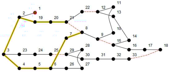
Figure 1.
Single-line diagram of the 33-bus network [19] showing the cycle formed by closing switch 21-8. Red node = feeder’s head; dashed red line = NO lines. Source: Author.
From one of the vertices of the NO tie switch, the BE heuristics verifies the next branches in the cycle, one by one, following a direction: the BE [16] suggests that operation must be performed first on the higher-voltage-drop side. So, in this example, the BE starts analyzing the way starting from the branch (7-8). The initial NO switch (21-8) is closed, the NC switch (7-8) is opened, and a fitness evaluation is performed. If the system losses decrease, the procedure continues to the other branches until no improvement is achieved. In this case, the NC switch that provided the lowest losses will be chosen as the new NO switch. The other direction of the cycle must be analyzed if no improvement occurs on the first one.
The procedure is repeated for each network NO switch, which corresponds to the number of basic cycles [46]. The BE application sequence in each cycle/NO switch will be detailed in Section 4.4.
4.2. The Iterative Branch Exchange
The proposed methodology consists of applying the BE heuristics within an iterative loop, which is inspired by the generation process used in evolutionary algorithms and population-based metaheuristics. The iterative BE is applied to the initial network configuration (i0). For each cycle/NO switch, if the BE is successful, a new individual is created and added to the population repository, which initially contains only the initial network configuration. Since the BE acts as a local search procedure in networks with more than one cycle, this approach can be classified as an iterative local search.
The elitism concept from evolutionary metaheuristics is also applied. Thus, on the next generation, the process is repeated, updating the last configuration analyzed (i0) with the elite individual from the population repository. Figure 2 presents the flowchart of the proposed methodology, also summarized in Algorithm 1. The iterative BE finishes when the stopping criteria, i.e., the maximum number of generations, is reached.
| Algorithm 1 Iterative Branch Exchange |
|
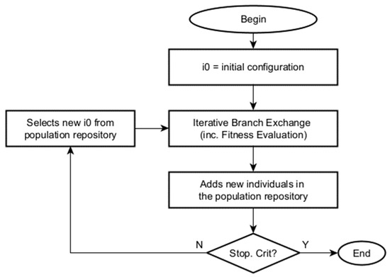
Figure 2.
Flowchart of the proposed iterative branch exchange.
4.3. Fitness Evaluation
The fitness evaluation step consists in evaluating the quality of the initial population and the new individuals created by the iterative BE. As long as the objective is the minimization of active power losses, the fitness value for each individual will be the power loss of its configuration. In the literature, the power losses are usually calculated using the power flow method, and the total power loss is calculated by summing up the active power losses in each line, as shown in (2).
In the literature, there are many power flow methods and algorithms, such as the Newton–Raphson [43] and Forward/Backward Sweep [47] methods. Currently, there are some open-source programs available, avoiding the cost of developing one from scratch, such as Matpower [43] and OpenDSS [44]. Matpower implements some traditional PF methods and the default solver is based on a standard Newton’s method. OpenDSS employs a nodal admittance formulation, also referred to as a current injection compensation method [48].
4.4. BE Application Sequence and Cycle Clusters
In the proposed methodology, the BE heuristics was applied in three different ways in relation to the order of choice of NO switches: (1) The NO switches with the largest cycles in the number of edges first; (2) the NO switches/cycles in random order; and (3) in each cycle cluster. The understanding of the first two is more straightforward and the explanation of the cycle cluster is given ahead.
In the scientific literature, cluster analysis is the task of grouping a set of objects in such a way that objects in the same group (called a cluster) are more similar (in some sense) to each other than to those in other groups (clusters) [34]. In this work, the cycle clustering is realized over the network connectivity graph defined in Section 4.1.
A cycle cluster is formed by two or more cycles in which one cycle is inside the other and therefore they share most of their edges. For example, Figure 3 shows a cycle cluster from the 136-bus network formed by the switches s145, s146, s154, and s155. Tie switches from adjacent clusters are also represented in this Figure.
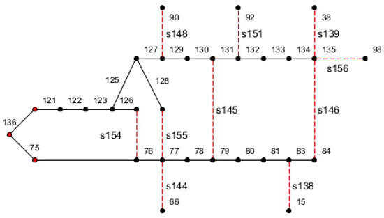
Figure 3.
136-bus network cycle cluster no. 4. Red nodes = feeder’s head; dashed red lines = NO lines. Source: Author.
The purpose of clustering the cycles is to reduce the search space of the heuristics, as the BE is applied in random order to each of the cycles of the analyzed cluster, while all other clusters are kept constant. The performance improvement with the clustering will be presented in Section 5 for the 136-bus network.
In this work, the clustering is performed by comparing the edges closest to the substation for each cycle. For instance, if two cycles have the same substation output edges, they will belong to the same cluster. One way to check this condition is to run any graph-traversal algorithm (again, the work used Dijkstra’s algorithm) twice for each cycle, from both nodes of the NO switch to the substation node. Then, the edges returned by the shortest paths are compared and all the cycles—named by their NO switches—are grouped according to the substation output edges. For example, Table 2 shows the grouping of 15 of the 21 NO switches of the 136-bus network, in its initial configuration, into 5 clusters.
Table 2.
NO switches for the 136-bus network grouped into 5 clusters.
5. Simulation and Results
5.1. Presentation of the Benchmark Systems
This Section presents the characteristics of the 33, 84, 70, and 136-bus networks with which the methodology was tested. Table 3 shows the main data about these systems: the number of buses, lines, and switches, the power losses for the initial and the optimal configuration, and their reference works. Table 4 shows the simulation parameters used in the iterative BE algorithm.
Table 3.
Overall data of the four test systems.
Table 4.
Simulation parameters.
Figure 4, Figure 5 and Figure 6 show the layouts of the 70-, 84-, and 136-bus networks, respectively.
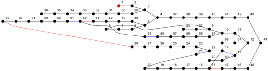
Figure 4.
Single-line diagram of 70-bus feeder [49]. Respectively: the red node represents the feeder’s head; dashed red lines = NO lines in the initial configuration; and blue lines will be NO lines in the optimal configuration (the NO 12-44 also belongs to the optimal configuration). Source: Author.
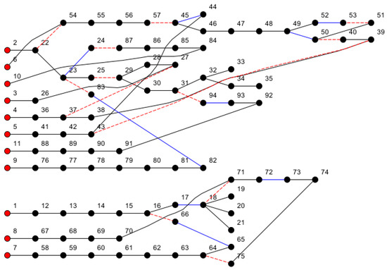
Figure 5.
Single-line diagram of the 84-bus feeders from Taiwan Power Company –TPC [11]. Respectively: red nodes represent the feeder’s head; dashed red line = NO lines in the initial configuration; and blue lines will be NO lines in optimal configuration (note that NOs 22-54, 25-29, 27-37, and 39-43 belong to both initial and optimal configuration). Source: Author.
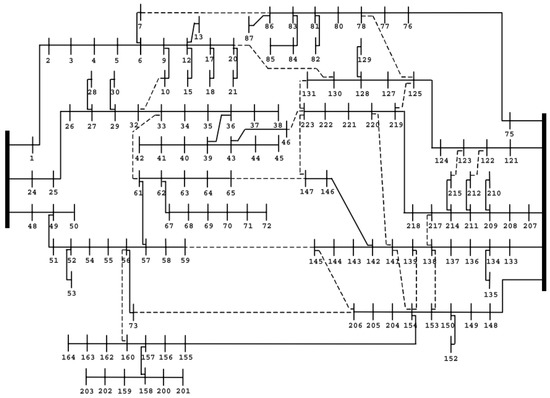
Figure 6.
Single-line diagram of the 136-bus system from Três Lagoas/MS—Brazil. Dashed lines = NO lines. Source [51].
5.2. Overall Numerical Results for Benchmark Systems
The proposed methodology presented 100% success, converging to the optimal solution in all ten simulation runs for the benchmark systems, the 33-, 84-, 70-, and 136-bus networks. Table 5 presents the results compared with other relevant works in the literature. For evolutionary metaheuristics works that did not report the NPF runs, it was estimated with , where is the population size and denotes the average number of iterations (in the worst case, if is not available it was substituted by G, the maximum number of generations). It is noteworthy that some works present an NPF lower than the proposed methodology, although only ref. [4] has also been tested in the four networks. Moreover, refs. [29,30] do not find the global optimum for the 136- and 84-bus networks, respectively.
Table 5.
Comparison of the proposed algorithm results with other relevant works in terms of the average NPF runs.
The results achieved are important to the field for showing that it is possible to minimize these networks starting from their original configuration—a feat that refs. [33] and [34] did not achieve. The results also show the superiority in the NPF runs of the methodology over the population-based evolutionary metaheuristics, which enables its application in larger real systems, as presented in Section 6.
5.3. Numerical Results—BE Application Order
Table 6 presents the results in terms of the NPF executions for two ways of applying the BE heuristics. In (1) the iterative BE is first applied to the largest cycles in the number of edges. In (2), the iterative BE is applied to the cycles in random order. The results show the effectiveness of the iterative BE in solving the DNRP for small-sized networks, such as the 33-, 70-, and 84-bus networks.
Table 6.
Variation in parameters for the proposed algorithm (average NPF executions in 10 runs).
5.4. Numerical Results—Cycle Cluster
This Section presents the numerical results for the cycle cluster. The cycle cluster was an approach to overcome the challenge of minimizing the 136-bus network, since, as presented in Section 5.3, the iterative BE minimized the 33-, 70-, and 84-bus networks effectively, but not the 136-bus network applying the two BE application sequences proposed in the last Section. When a cycle cluster, such as the one in Figure 3, is created, the algorithm performs an iterative BE internally in each cluster, choosing the NO switches in random order, while all other clusters are kept constant.
Measurement of the cycle cluster performance is complex since the number and size of clusters vary according to the analyzed individual [29]. However, the performance improvement can be shown by comparing the NPF between setup no. 2, from Section 5.3, with the BE sequence in random cycle order and setup no. 3, with cycle clustering. In addition, the number of successes in ten algorithm runs also demonstrates the performance improvement, since only two successes are obtained with setup no. 2. In the other eight runs, the algorithm became stuck in local minima. These results are summarized in Table 7. Due to the performance improvement in solving the 136-bus network, the authors encourage the use of CT in larger networks from the literature. Furthermore, future work should test computationally cheaper algorithms for graph traversal.
Table 7.
The performance improvement with the cycle cluster for the 136-bus network.
6. Case Studies: CEMIG-D Real Feeders
Unlike the benchmark networks that assume the existence of a tie switch in each distribution line, in real distribution feeders the total number of switches is much smaller than the number of line segments, and the distance between the switching devices is also greater. Nevertheless, the combinatorial analysis of all possibilities for these systems is very prohibitive. The upper bound is the binomial coefficient given by (11), where the number of NC and NO switches is shown in Table 8.
Table 8.
CEMIG-D feeders and substations numbers.
- is the total number of switches ();
- is the number of NO switches;
- is the number of NC switches.
Alternatively, a lower limit, which also gives an idea of the search space size for the DNRP, can be obtained with the number of spanning trees from a graph given by the Kirchhoff Matrix-Tree Theorem [38]. This theorem states that the number of spanning trees from graph G is given by any co-factor of the Laplacian matrix of G. This number is shown in Table 3 for the benchmark networks.
The proposed methodology was also implemented in a C#/OpenDSS [44] customization and was effective in minimizing the energy losses of CEMIG-D feeders. The OpenDSS power flow files were created from the database all Brazilian utilities are required to annually send to the regulatory agency. Document [52] establishes the parameters to model the feeders for the calculation of energy losses for Brazilian utilities. A requirement is to model the active loads as a mixed ZIP model with 50% constant power (P) and 50% constant impedance (Z). This load model and the existence of VRBs in the feeders required the addition of the constraint given by (10) and, thus, ensured that the transferred load would be supplied by a better voltage level. Section 6.3 presents a counter-example that details the motivation for the addition of this constraint.
The result from the OpenDSS customization is a list of switching operations sorted in a descending order of monthly energy loss reduction, in which the best switching operation was implemented in the field. Table 8 presents the characteristics of the four CEMIG-D feeders/substations, such as the number of NO and NC switches, buses, and both medium- and low-voltage clients.
Table 9 presents the energy loss reduction from these four reconfiguration cases over one month. For the calculation of the monthly energy losses, the methodology in [52] establishes that three daily power flows must be calculated, representing one business day, one Saturday, and one Sunday. In the OpenDSS, a daily power flow uses a load shape object for each load in the circuit, allowing a sequential-time power flow calculation. A load shape object consists of a series of multipliers, typically ranging between 0 and 1.0, applied to the load demand value and represents its variation over some period, in this case, a day. The results of the three daily power flows are weighted by the number of occurrences of each type of day in the month and summed together, thus obtaining the energy losses in a month [52]. Table 9 presents the estimation of the annual energy savings for the three reconfigurations carried out in the field. It must be taken into account that the dynamic of the actual distribution systems points to, at least, a quarterly review of the planning studies for energy loss minimization. In Table 9, the cost of performing the switching operations was not considered due to its low cost. For operations carried out by field teams, the estimated cost is USD100.00 per device, but some operations can be performed by remote control on IEDs. Finally, it also shows the voltage magnitude improvement with the reconfiguration, showing the voltages on NC switches before and after the maneuver.
Table 9.
Energy loss reduction and voltage level improvement for CEMIG-D reconfiguration cases.
6.1. Case Study no. 1: PSAU13 Feeder (Pouso Alegre City)
This is a typical case of load balancing. After the switching operation, represented in Figure 7 by the closing of NO switch no. 44055 (yellow circle) and the opening of NC switch no. 44169 (green circle), the total load is split between the two circuits. One load block gains access to the substation through switch no. 44055 at a distance of 1.99 km closer. In Figure 7, the other NO switches are represented by red circles.
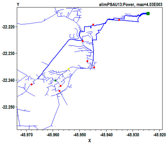
Figure 7.
PSAU13 feeder plot. The green square represents the substation; red circles = NO switches; green and yellow circles represent, respectively, the NC and NO switches before the maneuver. Source: Author.
In Figure 8, the switch operation is highlighted in a plot over the Google Earth map. The red circles highlight the NO and NC switches and the red line represents the feeder trunk before switching, while the light blue line represents the feeder trunk after the switching operation.
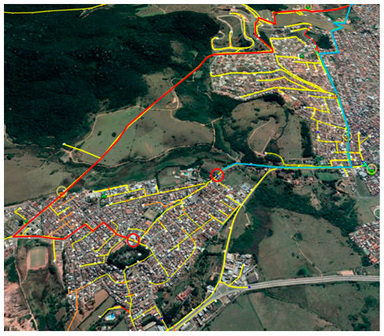
Figure 8.
IIGD substation switch operation—Link Google Maps. Source: Author.
6.2. Case Study No. 2: IIGD Substation (Ipatinga City)
This case presents a reconfiguration of an entire substation with more than 40,000 buses, which justifies the greatest NPF executions in Table 9. The best switching operation [close the NO switch no. 319112—yellow circle; open the NC switch no. 139164—green circle, in Figure 9] proposes feeding the loads through a shorter electrical path. Moreover, the switching operation was carried out by remote-controlled reclosers.
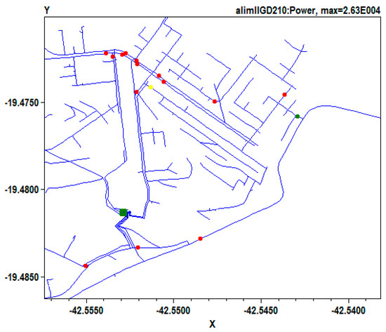
Figure 9.
IIGD substation plot. Green square = substation; red circles = NO switches; green and yellow circles represent, respectively, the NC and NO switches before the maneuver. Source: Author.
6.3. Case Study No. 3: IIGU115 Feeder (Belo Oriente City/MG)
This case is presented as a counter-example to explain the motivation for the addition of the voltage constraint given by (10). By running the algorithm without this constraint, the solution would propose the following maneuver: [close the NO switch no. 130817—yellow circle; open the NC switch no. 48676—green circle, in Figure 10].
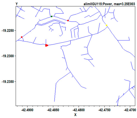
Figure 10.
IIGU115 feeder plot. The red triangle represents the VRB; red circles = NO switches; green and yellow circles represent respectively the NC and NO of the proposed maneuver. Source: Author.
Table 10 shows the voltage level at peak load hour (6 pm), on the NC switches before and after the proposed maneuver. Thus, the reduction in energy losses would occur due to the 0.017 p.u. voltage level reduction on the normally closed switches due to the bypassing of VRB no. 141495—red triangle in Figure 10.
Table 10.
The simulated voltage level at the NC switches before and after the proposed maneuver.
Discussion: Since the real feeder usually includes voltage-dependent loads, the voltage level constraint given by (10) guarantees that the transferred load will be supplied at an equal or higher voltage level, preventing the undesirable side-effect of the VRBs being bypassed by other electrical paths, as shown in this case study. In addition, the voltage level constraint avoids the VRB bypass caused by its own bypass switches, since in the modeling of real feeders they are usually represented, as exemplified in Figure 11.
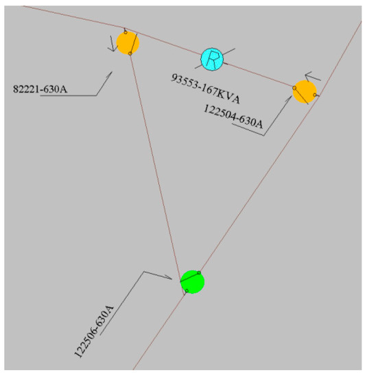
Figure 11.
The VRB no. 93553 and its bypass switches no. 122504 and no. 122506, normally opened, are represented in green color. The arrows represent the power flow direction. Source: Author.
6.4. Case Study No. 4: CETU Substation (Caeté City/MG)
This case presents a reconfiguration of another substation with more than 30,000 buses. The methodology discovered the possibility of feeding the loads through a more robust and reliable network. After the switching operation [close the NO switch no. 302068; open the NC switch no. 257774, in Figure 12, the loads are fed by protected cables instead of conventional 4/0 AWG cables (.
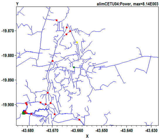
Figure 12.
CETU substation plot. Green square = substation; red circles = NO switches; green circle = NC switch; yellow circle = NO switch to be closed. Source: Author.
Discussion: The case studies demonstrate both the reduction in energy losses and the improvement of the voltage level in real distribution feeders (Table 9). In most reconfiguration cases, the reduction in losses results from feeding through thicker conductors (e.g., “bottleneck” elimination) and/or feeding by shorter electrical paths.
Taking into consideration the size of real feeders and substations, the amount of NO and NC switches, and therefore the size of the search space as presented in Table 8, the iterative BE proved to be suitable for minimizing losses on real distribution networks within a reasonable NPF. A contribution to the low NPF is the fact that the methodology does not require the creation of an initial population of candidate solutions, which usually requires special algorithms as well as the expenditure of computational resources for the fitness evaluation of this population. So far, it has been applied to 81 reconfiguration cases for CEMIG-D with a total simulated energy loss reduction of more than 3.600 MWh/year. The current characteristics of the modern distribution systems, such as the number of DERs and IEDs in the grid, point to at least a quarterly review of the planning studies for energy loss minimization.
As the switching operations are performed within the same substation, the short-circuit level does not change. In addition, the reliability indexes (e.g., SAIDI, SAIFI) are often improved after the operation, because the loads are supplied by networks closer to the substation or conventional distributed networks changed by protected or isolated ones, as shown in case study no. 4. For future work, the inclusion of reliability indexes in the mathematical optimization model will be considered. In this way, the execution of maneuvers into more reliable networks will be prioritized.
7. Conclusions
This work demonstrated that the association of branch exchange heuristics with evolutionary metaheuristics concepts is a practical combination to solve the DNRP. The use of iterative BE proved to be capable of optimizing 33-, 70-, 84-, and 136-bus networks using only the original configuration as a starter solution. The results in the NPF runs for these networks are on the same order of magnitude as those in other works about BE heuristics and are significantly better than the approaches with population-based evolutionary metaheuristics. One of the advantages of this methodology over population-based evolutionary metaheuristics is that it does not demand the creation of an initial population of candidate solutions, which enables its application in larger real systems and even in real-time reconfiguration.
The methodology was applied to real 13.8 kV distribution feeders and entire substations with more than 43,000 buses from CEMIG-D. The work considered the existence of voltage-dependent loads and presented the undesirable effect of voltage regulator bank by-passing and the way this problem was tackled through the addition of the voltage-level constraint on the NC switches. The four case studies showed that a lower loss configuration was discovered with a low number of PF runs, thus enabling the methodology to be employed by distribution utilities to reconfigure real distribution feeders.
Supplementary Materials
All the source codes and Supplementary Materials are published in the following repository: https://github.com/Zecao/IterativeBranchExchange (accessed on 4 February 2023). Please see the Data Availability Statement below.
Author Contributions
Conceptualization, E.C.P.; Methodology, E.C.P., C.H.N.R.B. and J.A.V.; Software, E.C.P.; Validation, E.C.P.; Investigation, E.C.P.; Writing—original draft, E.C.P.; Writing—review & editing, E.C.P., C.H.N.R.B. and J.A.V.; Supervision, J.A.V. All authors have read and agreed to the published version of the manuscript.
Funding
This research received no external funding.
Data Availability Statement
In the following repository, https://github.com/Zecao/IterativeBranchExchange, one will find 1. the MATLAB codes for the replication of the results; 1.1 a spreadsheet with the results of each of the ten iterative BE runs for the 33-, 70-, 84- and 136-bus networks; 2. the OpenDSS C# customization codes; 3. the OpenDSS files (.dss) for the four case studies presented and instructions; and 4. other extra materials.
Acknowledgments
The authors would like to thank the company CEMIG Distribuição S.A. for supporting the development of the OpenDSS customization, as well as the operation and field teams that carried out the reconfigurations mentioned in the work.
Conflicts of Interest
The authors declare no conflict of interest.
References
- Mishra, S.; Das, D.; Paul, S. A comprehensive review on power distribution network reconfiguration. Energy Syst. 2017, 8, 227–284. [Google Scholar] [CrossRef]
- Ababei, C.; Kavasseri, R. Efficient network reconfiguration using minimum cost maximum flow-based branch exchanges and random walks-based loss estimations. IEEE Trans. Power Syst. 2011, 26, 30–37. [Google Scholar] [CrossRef]
- Raju, G.K.V.; Bijwe, P.R. An efficient algorithm for minimum loss reconfiguration of distribution system based on sensitivity and heuristics. IEEE Trans. Power Syst. 2008, 23, 1280–1287. [Google Scholar] [CrossRef]
- Zin, A.A.M.; Ferdavani, A.K.; Bin Khairuddin, A.; Naeini, M.M. Two circular-updating hybrid heuristic methods for minimum-loss reconfiguration of electrical distribution network. IEEE Trans. Power Syst. 2013, 28, 1318–1323. [Google Scholar] [CrossRef]
- Shaheen, A.; El-Sehiemy, R.; Kamel, S.; Selim, A. Optimal Operational Reliability and Reconfiguration of Electrical Distribution Network Based on Jellyfish Search Algorithm. Energies 2022, 15, 6994. [Google Scholar] [CrossRef]
- Barbosa, C.H.N.D.R.; Alexandre, R.F.; de Vasconcelos, J.A. A practical codification and its analysis for the generalized reconfiguration problem. Electr. Power Syst. Res. 2013, 97, 19–33. [Google Scholar] [CrossRef]
- Alanazi, A.; Alanazi, M. Artificial Electric Field Algorithm-Pattern Search for Many-Criteria Networks Reconfiguration Considering Power Quality and Energy Not Supplied. Energies 2022, 15, 5269. [Google Scholar] [CrossRef]
- TRACTEBEL. Identifying Energy Efficiency Improvements and Saving Potential in Energy Networks, Including Analysis of the Value of Demand Response; European Commission: Brussels, Belgium, 2015. [Google Scholar]
- Beza, T.M.; Huang, Y.C.; Kuo, C.C. A hybrid optimization approach for power loss reduction and dg penetration level increment in electrical distribution network. Energies 2020, 13, 6008. [Google Scholar] [CrossRef]
- Cheng, S.; Li, Z. Multi-Objective Network Reconfiguration Considering v2g of Electric Vehicles in Distribution System with Renewable Energy. Energy Procedia 2019, 158, 278–283. [Google Scholar] [CrossRef]
- Alwash, S.; Ibrahim, S.; Abed, A.M. Distribution System Reconfiguration with Soft Open Point for Power Loss Reduction in Distribution Systems Based on Hybrid Water Cycle Algorithm. Energies 2023, 16, 199. [Google Scholar] [CrossRef]
- Xu, J.; Zhang, T.; Du, Y.; Zhang, W.; Yang, T.; Qiu, J. Islanding and dynamic reconfiguration for resilience enhancement of active distribution systems. Electr. Power Syst. Res. 2020, 189, 106749. [Google Scholar] [CrossRef]
- Gharebaghi, S.; Izadi, M.; Safdarian, A. Optimal Network Configuration Considering Network Losses and Service Reliability. In Proceedings of the 2017 Smart Grid Conference (SGC), Tehran, Iran, 20–21 December 2017. [Google Scholar]
- Tranberg, B.; Corradi, O.; Lajoie, B.; Gibon, T.; Staffell, I.; Andresen, G.B. Real-Time Carbon Accounting Method for the European Electricity Markets. Energy Strategy Rev. 2019, 26, 100367. [Google Scholar] [CrossRef]
- Kumar, K.K.; Ramana, N.V.; Kamakshaiah, S.; Nishanth, P.M. State of art for network reconfiguration methodologies of distribution system. J. Theor. Appl. Inf. Technol. 2013, 57, 25–40. [Google Scholar]
- Civanlar, S.; Grainger, J.J.; Yin, H.; Lee, S.S.H. Distribution Feeder Reconfiguration for Loss Reduction. IEEE Trans. Power Deliv. 1988, 3, 1217–1223. [Google Scholar] [CrossRef]
- Baran, M.E.; Wu, F.F. Network reconfiguration in distribution systems for loss reduction and load balancing. IEEE Trans. Power Deliv. 1989, 4, 1401–1407. [Google Scholar] [CrossRef]
- Merlin, A.; Back, H. Search for a Minimal—Loss Operating Spanning Tree Configuration in an Urban Power Distribution System. In Proceedings of the 5th Power System Conference, London, UK, 1–5 September 1975. [Google Scholar]
- Zhu, J.Z. Optimal reconfiguration of electrical distribution network using the refined genetic algorithm. Electr. Power Syst. Res. 2002, 62, 37–42. [Google Scholar] [CrossRef]
- Shirmohammadi, D.; Hong, H.W. Reconfiguration of electric distribution networks for resistive line losses reduction. IEEE Trans. Power Deliv. 1989, 4, 1492–1498. [Google Scholar] [CrossRef]
- McDermott, T.E.; Drezga, I.; Broadwater, R.P. A Heuristic Nonlinear Constructive Method. IEEE Trans. Power Syst. 1999, 14, 478–483. [Google Scholar] [CrossRef]
- de Macedo Braz, H.D.; de Souza, B.A. Distribution network reconfiguration using genetic algorithms with sequential encoding: Subtractive and additive approaches. IEEE Trans. Power Syst. 2011, 26, 582–593. [Google Scholar] [CrossRef]
- Wang, C.; Gao, Y. Determination of power distribution network configuration using non-revisiting genetic algorithm. IEEE Trans. Power Syst. 2013, 28, 3638–3648. [Google Scholar] [CrossRef]
- Tiguercha, A.; Ladjici, A.A.; Boudour, M. Optimal Radial Distribution Network Reconfiguration Based on Multi Objective Differential Evolution Algorithm. In Proceedings of the 2017 IEEE Manchester PowerTech, Manchester, UK, 18–22 June 2017. [Google Scholar] [CrossRef]
- Pegado, R.; Ñaupari, Z.; Molina, Y.; Castillo, C. Radial distribution network reconfiguration for power losses reduction based on improved selective BPSO. Electr. Power Syst. Res. 2019, 169, 206–213. [Google Scholar] [CrossRef]
- Alonso, G.; Alonso, R.; de Souza, A.C.Z.Z.; Freitas, W. Enhanced Artificial Immune Systems and Fuzzy Logic for Active Distribution Systems Reconfiguration. Energies 2022, 15, 9419. [Google Scholar] [CrossRef]
- Carreño, E.M.; Romero, R.; Padilha-Feltrin, A. An efficient codification to solve distribution network reconfiguration for loss reduction problem. IEEE Trans. Power Syst. 2008, 23, 1542–1551. [Google Scholar] [CrossRef]
- Queiroz, L.M.O.; Lyra, C. Adaptive hybrid genetic algorithm for technical loss reduction in distribution networks under variable demands. IEEE Trans. Power Syst. 2009, 24, 445–453. [Google Scholar] [CrossRef]
- Gupta, N.; Swarnkar, A.; Niazi, K.R. A Modified Branch-Exchange Heuristic Algorithm for Large-Scale Distribution Networks Reconfiguration. In Proceedings of the 2012 IEEE Power and Energy Society General Meeting, San Diego, CA, USA, 22–26 July 2012; pp. 1–7. [Google Scholar] [CrossRef]
- Zin, A.A.M.; Ferdavani, A.K.; Bin Khairuddin, A.; Naeini, M.M. Reconfiguration of radial electrical distribution network through minimum-current circular-updating-mechanism method. IEEE Trans. Power Syst. 2012, 27, 968–974. [Google Scholar] [CrossRef]
- Souza, S.S.F.; Romero, R.; Pereira, J.; Saraiva, J.T. Reconfiguration of Radial Distribution Systems with Variable Demands Using the Clonal Selection Algorithm and the Specialized Genetic Algorithm of Chu-Beasley. J. Control Autom. Electr. Syst. 2016, 27, 689–701. [Google Scholar] [CrossRef]
- Souza, S.S.F.; Romero, R.; Pereira, J.; Saraiva, J.T. Artificial immune algorithm applied to distribution system reconfiguration with variable demand. Int. J. Electr. Power Energy Syst. 2016, 82, 561–568. [Google Scholar] [CrossRef]
- Salazar, H.; Gallego, R.; Romero, R. Artificial neural networks and clustering techniques applied in the reconfiguration of distribution systems. IEEE Trans. Power Deliv. 2006, 21, 1735–1742. [Google Scholar] [CrossRef]
- Fathabadi, H. Power distribution network reconfiguration for power loss minimization using novel dynamic fuzzy c-means (dFCM) clustering based ANN approach. Int. J. Electr. Power Energy Syst. 2016, 78, 96–107. [Google Scholar] [CrossRef]
- Cao, H.; Gao, C.; Chen, P.; He, X.; Dong, Z.; Lin, L. Distribution Network Dynamic Reconfiguration Based on Improved Fuzzy C-Means Clustering with Time Series Analysis. IEEJ Trans. Electr. Electron. Eng. 2022, 17, 174–182. [Google Scholar] [CrossRef]
- Ji, X.; Zhang, X.; Zhang, Y.; Yin, Z.; Yang, M.; Han, X. Three-phase symmetric distribution network fast dynamic reconfiguration based on timing-constrained hierarchical clustering algorithm. Symmetry 2021, 13, 1479. [Google Scholar] [CrossRef]
- Ahmadi, H.; Martí, J.R. Minimum-loss network reconfiguration: A minimum spanning tree problem. Sustain. Energy Grids Netw. 2015, 1, 1–9. [Google Scholar] [CrossRef]
- Macedo, L.H.; Franco, J.F.; Mahdavi, M.; Romero, R. A Contribution to the Optimization of the Reconfiguration Problem in Radial Distribution Systems. J. Control Autom. Electr. Syst. 2018, 29, 756–768. [Google Scholar] [CrossRef]
- Jakus, D.; Čađenović, R.; Vasilj, J.; Sarajčev, P. Optimal reconfiguration of distribution networks using hybrid heuristic-genetic algorithm. Energies 2020, 13, 1544. [Google Scholar] [CrossRef]
- Lavorato, M.; Franco, J.F.; Rider, M.J.; Romero, R. Imposing radiality constraints in distribution system optimization problems. IEEE Trans. Power Syst. 2012, 27, 172–180. [Google Scholar] [CrossRef]
- ANEEL. Procedimentos de Distribuição de Energia Elétrica no Sistema Elétrico Nacional—PRODIST—Módulo 8—Qualidade da Energia Elétrica; Agência Nacional de Energia Elétrica: Brasília, Brazil, 2018.
- Gaspar, W.A.; de Oliveira, E.J.; Garcia, P.A.N.; Amaral, M.B.D. Static Load Model Adjustment using Fuzzy Logic and Differential Evolution. In Proceedings of the 2012 10th IEEE/IAS International Conference on Industry Applications, INDUSCON 2012, Fortaleza, Brazil, 5–7 November 2012. [Google Scholar] [CrossRef]
- Zimmerman, R.D.; Murillo-Sanchez, C.E.; Thomas, R.J. MATPOWER: Steady-State Operations, Planning, and Analysis Tools for Power Systems Research and Education. IEEE Trans. Power Syst. 2011, 26, 12–19. [Google Scholar] [CrossRef]
- EPRI. Simulation Tool—OpenDSS. 2023. Available online: https://www.epri.com/pages/sa/opendss?lang=en (accessed on 17 February 2023).
- Dijkstra, E.W. A Note on Two Problems in Connexion with Graphs. Numer. Math. 1959, 1, 269–271. [Google Scholar] [CrossRef]
- Mendoza, J.; López, R.; Morales, D.; López, E.; Dessante, P.; Moraga, R. Minimal loss reconfiguration using genetic algorithms with restricted population and addressed operators: Real application. IEEE Trans. Power Syst. 2006, 21, 948–954. [Google Scholar] [CrossRef]
- Shirmohammadi, D.; Hong, H.W.; Semlyen, A.; Luo, G.X. A Compensation-based Power Flow Method for Weakly Meshed Distribution and Transmission Networks. IEEE Trans. Power Syst. 1988, 3, 753–762. [Google Scholar] [CrossRef]
- Rocha, C.; Radatz, P. Algoritmo de Fluxo de Potência do OpenDSS. Electr. Power Syst. Res. 2017, 1–24. [Google Scholar]
- Huang, Y.-C. Enhanced genetic algorithm-based fuzzy multi-objective approach to distribution network reconfiguration. IEEE Proc. Gener. Transm. Distrib. 2002, 149, 615–620. [Google Scholar] [CrossRef]
- Su, C.-T.; Lee, C.-S. Network reconfiguration of distribution systems using improved mixed-integer hybrid differential evolution. IEEE Trans. Power Deliv. 2003, 18, 1022–1027. [Google Scholar] [CrossRef]
- Mantovani, J.R.S.; Casari, F.; Romero, R.A. Reconfiguração de sistemas de distribuição radiais utilizando o critério de queda de tensão. SBA Controle Autom. 2000, 11, 150–159. [Google Scholar]
- ANEEL. PRODIST—Módulo 7—Cálculo de Perdas na Distribuição; Agência Nacional de Energia Elétrica: Brasília, Brazil, 2015.


Disclaimer/Publisher’s Note: The statements, opinions and data contained in all publications are solely those of the individual author(s) and contributor(s) and not of MDPI and/or the editor(s). MDPI and/or the editor(s) disclaim responsibility for any injury to people or property resulting from any ideas, methods, instructions or products referred to in the content. |
© 2023 by the authors. Licensee MDPI, Basel, Switzerland. This article is an open access article distributed under the terms and conditions of the Creative Commons Attribution (CC BY) license (https://creativecommons.org/licenses/by/4.0/).