
Capacity Optimization of Independent Microgrid with Electric Vehicles Based on Improved Pelican Optimization Algorithm
Abstract
:1. Introduction
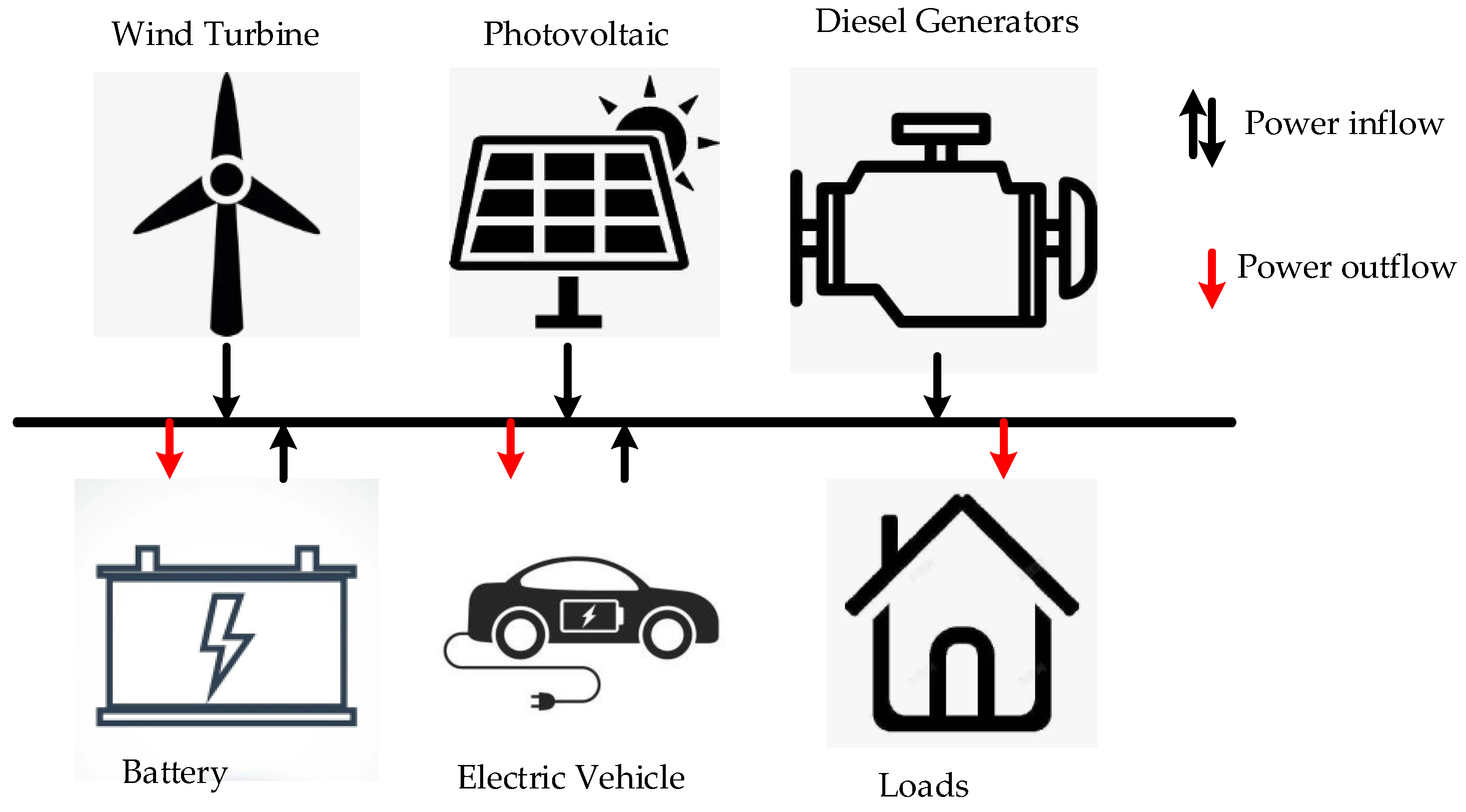
2. Basic Model
2.1. Microgrid Model
2.1.1. Wind Power Output
2.1.2. Solar Power Output
2.1.3. BESS Power Output
2.1.4. DIE Power Output
2.2. Load Characteristic
2.3. Electric Vehicle Charging and Discharging Model
2.3.1. Non-Dispatchable Electric Vehicles
2.3.2. Dispatchable Electric Vehicles
2.3.3. Constraints and Power Balance Constraints
2.4. Incentive Demand Response
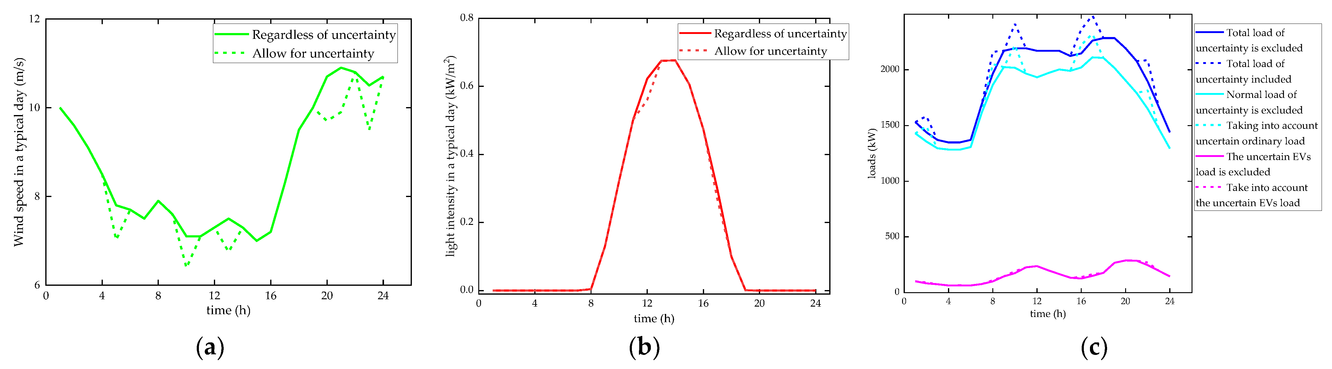
2.5. Uncertainty
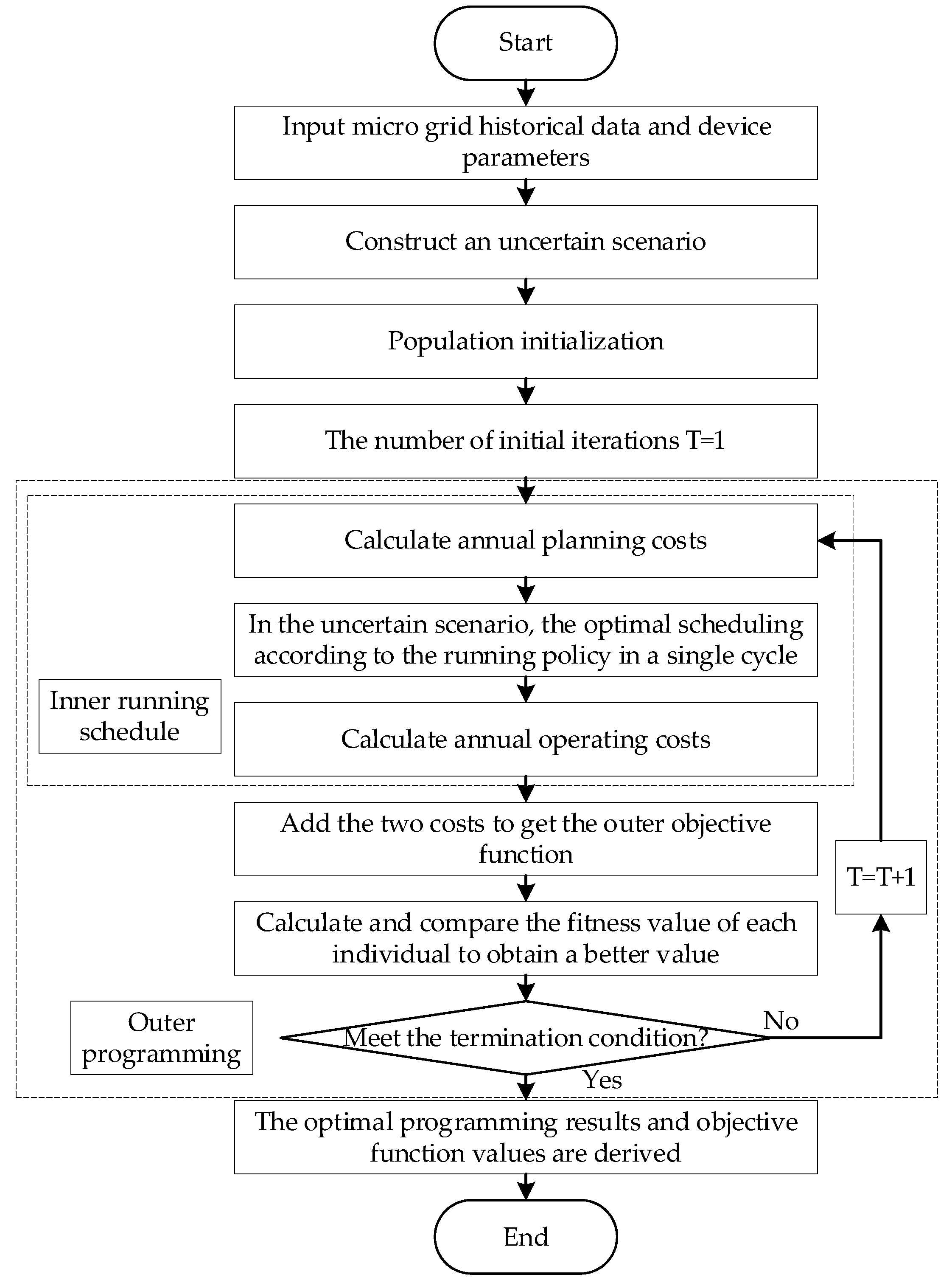
3. Capacity Optimization Model
3.1. Upper-Level Model
- (1)
- The average annual investment cost is related to the equipment’s first investment cost and the system’s operating life.where is the power cost coefficient of each distributed power supply; ni is the number of installed power supplies; is the rated power of each power supply; ηcrf is the fund recovery coefficient. a is the effective interest rate; Y is the whole life of the system, and 20 years was taken in this paper. a′ is the rated interest rate, 8% in this paper; y is the annual inflation rate, 5% in this paper.
- (2)
- Average annual equipment operation and maintenance expenses are related to operation and maintenance costs in the first year.where is each power supply’s operation and maintenance cost coefficient.
- (3)
- The average annual replacement cost is related to the service life of each distributed power source.where Li is the replacement times of each power supply within the system life.
3.2. Lower-Level Model
- (1)
- The independent microgrid considered in this paper consumes fuel only when the diesel generator runs, and the fuel cost is generated only by the diesel engine.where koil is the fuel cost coefficient of the diesel generator, and Pdie(t) is the actual operating power of the diesel generator.
- (2)
- A diesel engine will emit CO2, SO2, NOx, and other polluting gases during operation. To unify the dimension, this must be converted into pollution control costs for treatment. Pollution control cost CP is related to the output power of the diesel generator:where is the emission coefficient of different pollutants, and is the treatment cost coefficient of different pollutants.
- (3)
- Due to the randomness of scenery resources, there will be some problems, such as wind and light abandonment during the operation of the system; that is, the power output of the microgrid system will be greater than the power demand, which leads to energy waste and a decrease in the utilization rate of renewable energy. Energy waste penalty cost CW is introduced here to measure the utilization rate of renewable energy in the system:where kwas is the penalty cost coefficient, and Pwas(t) is the power of energy surplus.
- (4)
- The total cost CDR of the incentive type includes the compensation cost CDR,1 and CDR,2 of the shiftable load and dispatchable EV to users, and the cost CDR,3 of the microgrid to purchase electricity from dispatchable EV users, which is expressed as follows:where a1, a2, and a3 are the compensation costs of unit electricity transferred by shiftable load, dispatchable EV, and the cost of unit electricity purchased by the microgrid, respectively.
3.3. Constraint Condition
- (1)
- Because the area available for the installation of distributed power devices in the microgrid is limited, the number of power supplies to be installed should meet the constraints
- (2)
- The battery’s life is related to whether it is deeply discharged. Overcharging or overdischarging will reduce the battery life. In order to extend the service life of the battery, the charging and discharging power and the state of charge of the battery should meet the constraints
- (3)
- The power deficit constraint and the reliability of the system are represented by the size of the system power deficit; a low power deficit will not cause a more significant impact on production and life. In this paper, the maximum power deficit rate of the system was set at 0.1%; that is, the power deficit cannot exceed 0.1% of the total load of the system. The power deficit rate ksho can be calculated as follows:where Pi(t) is the power of each power supply at time t; Pfh(t) is the power at time t of the load; PFH is the total annual load.
- (4)
- The environmental protection index of the system is represented by the emission of pollutants at the power generation end of the system. The only pollution source of the microgrid system considered in this paper was the pollutant emission from diesel generators. In order to ensure the environmental protection requirements of the microgrid, pollutant emissions generated by the operation of diesel generators need to be controlled. In this paper, pollution control costs were used for restraint, and the maximum pollution control cost in this paper was set at CNY 1 million.where is the maximum pollution control cost of the system.
3.4. Microgrid Operation Control Strategy
4. Model-Solving Method
4.1. Pelican Optimization Algorithm
- (1)
- Move toward prey (exploration phase).
- (2)
- Wingspan above water (development stage).
4.1.1. Phase 1: Move to Prey (Exploration Phase)
4.1.2. Phase 2: Flying over Water (Development Phase)
4.2. Improved Pelican Optimization Algorithm
4.2.1. Population Initialization Based on Stochastic Opposition Learning
4.2.2. Disturbance Suppressor
4.2.3. Lévy Flight Strategy
4.3. IPOA Algorithm Flow Chart and Pseudo-Code
| Algorithm 1. Pseudo-code of IPOA |
| Start IPOA 1. Enter the optimization problem information. 2. Determine the overall size of IPOA (N) and the number of iterations (T). 3. Initialize the pelican position and calculate the objective function. 4. Update the pelican position and calculate the objective function using Equation (35). 5. Locate the pelican using Equation (36). 6. For t = 1:T 7. Randomly generate prey positions. 8. For i = 1:N 9. Phase 1: Moving toward prey (exploration stage). 10. For j = 1:m 11. Calculate the new state of the j-th dimension using Equation (38). 12. End 13. Update the ith population member using Equation (32). 14. Phase 2: Flying over water (development phase). 15. For j = 1:m. 16. Calculate the new state of dimension j using Equation (39). 17. End 18. Update the i-th population member using Equation (34). 19. Calculate the new state of dimension j using Equation (40). 20. Update the i-th population member using Equation (34). 21. End 22. Update the best candidate solutions. 23. End. 24. Output the best candidate solution obtained through IPOA. End IPOA. |
5. Example Analysis
5.1. Basic Data and Parameter Settings
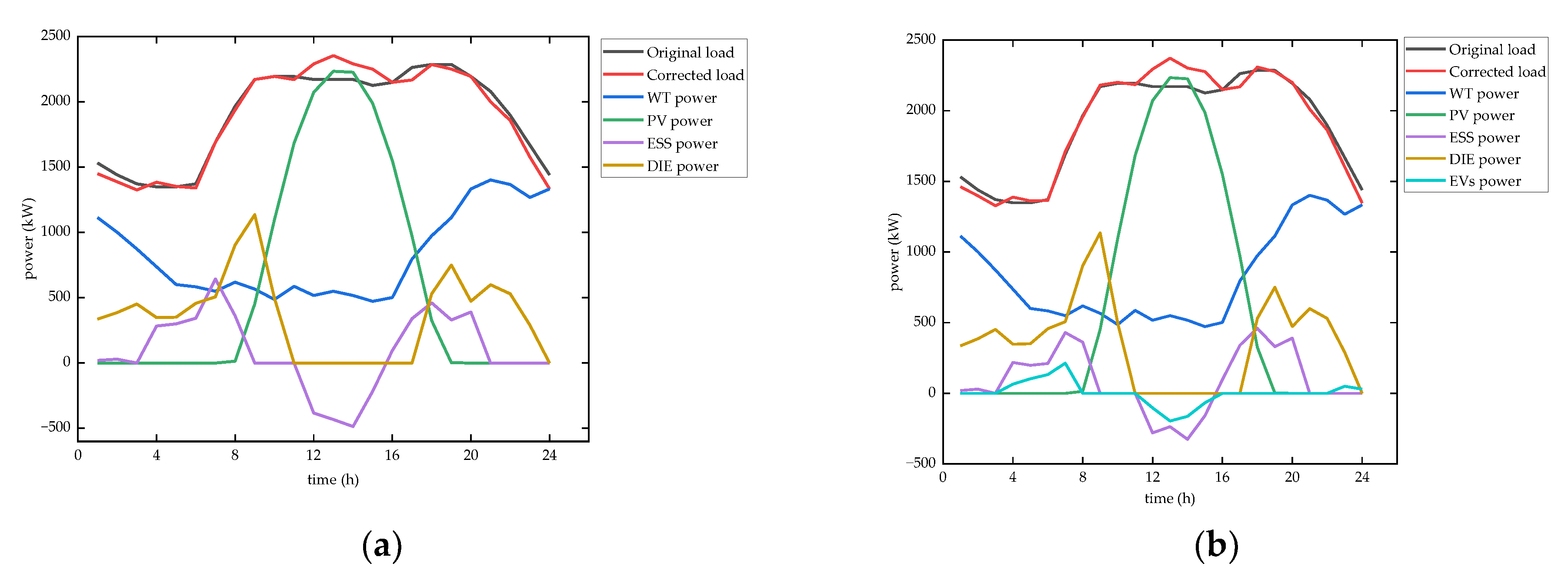
5.2. Analysis and Comparison of Different Influencing Factors
5.3. Comparative Analysis of IPOA and Other Algorithms
6. Summary of the Main Results
7. Conclusions
- (1)
- This paper constructed an independent microgrid capacity optimization configuration model that included electric vehicles. By introducing electric vehicles and including dispatchable electric vehicles in the incentive DR, the total cost and investment cost of the power capacity optimization of the microgrid were reduced compared with the traditional model. Because of the energy storage characteristics of dispatchable electric vehicles, the number of energy storage equipment construction configurations was significantly reduced. The example analysis found that the capacity optimization cost of the microgrid was reduced by CNY 139,633 after considering electric vehicles.
- (2)
- The capacity optimization allocation method of the independent microgrid proposed in this paper considered uncertainty and the DR. When the uncertainty of the source load was considered, the user comfort level was taken into account, and the uncertain influence of the shifting load and dispatchable EV load was fully considered. The optimal configuration model of the independent microgrid was further improved, and the calculated configuration results were more reasonable.
- (3)
- An improved pelican optimization algorithm was proposed. In view of the problems with the traditional pelican optimization algorithm, such as uneven initial population distribution and easily falling into the local optimum, improved methods such as the stochastic opposition learning strategy, disturbance inhibition factor, and Lévy flight strategy were proposed to improve the initial population and increase the convergence rate, the global search ability, and the solution stability. After the POA improved, the capacity optimization cost of the microgrid was reduced by CNY 49,601.
Author Contributions
Funding
Data Availability Statement
Conflicts of Interest
Nomenclature
| BESS | battery energy storage system |
| maximum pollution control cost of the system | |
| Cinv | annual planning cost of micro-network construction by operators |
| Cnei | annual operating cost of the system |
| Cini | average annual investment cost |
| Cmain | annual maintenance cost |
| Ccha | annual replacement cost |
| Cfuel | fuel cost of DIE |
| CP | pollution control cost of the system |
| CW | renewable energy waste penalty cost |
| CDR | compensation cost for incentive DR |
| DIE | diesel generator |
| DR | demand response |
| EV | electric vehicle |
| EVs | electric vehicles |
| Foil | fuel consumption of the DIE |
| GAC | light intensity |
| kwas | penalty cost coefficient |
| k | power temperature coefficient |
| emission coefficient of different pollutants | |
| treatment cost coefficient of different pollutants | |
| koil | fuel cost coefficient of the DIE |
| power cost coefficient of each distributed power supply | |
| each power supply’s operation and maintenance cost coefficient | |
| kdie1 | intercept coefficient of the fuel curve |
| kdie2 | slope of the fuel curve |
| Li | replacement times of each power supply within the system life |
| ηd | discharge efficiency |
| ηc | charging efficiency |
| ni | number of installed power supplies |
| ηcrf | fund recovery coefficient |
| ηEV | total number of EVs |
| ηgEV | number of undispatchable EVs |
| ηkEV | number of dispatchable EVs |
| ηEV,D | discharging coefficients of EVs |
| ηEV,C | charging coefficients of EVs |
| nEVmin | minimum coefficients |
| nEVmax | maximum coefficients |
| Ni,t | degree of uncertainty |
| Δt | unit of an hour |
| Pc(t) | charging amount in unit time △t |
| Pd(t) | discharge quantity in unit time △t |
| Pwas(t) | power of energy surplus |
| Pi(t) | power of each power supply at time t |
| Pfh(t) | power at time t of load |
| PFH | total annual load |
| Ppv | output power of PV |
| Pwt(t) | power of a WT |
| PSTC | maximum test power under standard test conditions |
| Pdie(t) | actual operating power of the DIE |
| rated power of each power supply | |
| Pzy(t) | total load transfer power |
| Pzyo(t) | transfer power of shifting load |
| PzyEV(t) | transfer power of dispatchable EV |
| PKEV,D(t) | discharge power of EVs |
| PKEV,C(t) | charging power of EVs |
| PKEV,h(t) | energy consumption power of EVs |
| PEV(t) | power of EVs |
| PgEV(t) | power of undispatchable EVs |
| PkEV(t) | power of dispatchable EVs |
| Pzfh(t) | total load power within a unit of time |
| Pgfh(t) | rigid load power within a unit of time |
| Pkfh(t) | translational load power within a unit of time |
| rated power of the DIE | |
| Pdie | actual output power of the DIE |
| Po | rated power of the WT |
| PV | photovoltaic |
| POA | pelican optimization algorithm |
| IPOA | improved pelican optimization algorithm |
| SOC | state of charge |
| SEV(t) | capacity of the EV at time t |
| SEVmin | minimum of SEV(t) |
| SEVmax | maximum of SEV(t) |
| SEV | total capacity of EVs |
| SgEV | total capacity of non-schedulable EVs |
| SkEV | total capacity of schedulable EVs |
| SEVO | capacity of a single EV |
| SzyEV(t) | power supply of the EV to the microgrid within a unit of time |
| Tr | reference temperature |
| Tc | operating temperature of the panel |
| Tamt | ambient temperature |
| ui,t | value of time period t of 6 uncertain variables |
| ufor,i,t | predicted values of uncertain variables |
| v | wind speed at time period t of the WT |
| vl | input-wind speed |
| vo | rated wind speed |
| vu | cut-out wind speed |
| WT | wind turbine |
| xi,t | maximum prediction error of uncertain variable |
References
- Balaguer, I.J.; Lei, Q.; Yang, S.; Supatti, U.; Peng, F.Z. Control for Grid-Connected and Intentional Islanding Operations of Distributed Power Generation. IEEE Trans. Ind. Electron. 2011, 58, 147–157. [Google Scholar] [CrossRef]
- Anderson, B.; Rane, J.; Khan, R. Distributed wind-hybrid microgrids with autonomous controls and forecasting. Appl. Energy 2023, 333, 120557. [Google Scholar] [CrossRef]
- Hu, Z.; Zhan, K.; Xu, Z.; Xing, D.; Zhang, H. Analysis and Outlook on the Key Problems of Electric Vehicle and Power Grid Interaction. Electr. Power Constr. 2015, 36, 6–13. [Google Scholar]
- Yang, J.; Wen, F.; Wang, Z.; Zhang, X.; Wang, L.; Zeng, P. Interactions between Electric Wehicles and Power Systems. Electr. Power Constr. 2015, 36, 14–24. [Google Scholar]
- Peng, Q.; Wang, X.; Shi, S.; Wang, S.; Yan, S.; Chen, Y. Multi-objective Planning of Microgrid Considering Electric Vehicles Charging Load. In Proceedings of the 5th Asia Conference on Power and Electrical Engineering (ACPEE), Chengdu, China, 4–7 June 2020. [Google Scholar]
- Yang, L.; Yang, B.; An, L.; Cao, Y.; Liang, J. Optimal Configuration of Grid-Connected Pv-And-Storage Microgrid Considering Evs’Demand Response. Acta Energ. Sol. Sin. 2020, 41, 340–347. [Google Scholar]
- Lin, Y.; Wang, K.; Quan, M.; Zhang, Z.; Dong, X. Optimal Allocation Method for Microgrid System Capacity with Electrical Vehicles. In Proceedings of the 2021 6th International Conference on Power and Renewable Energy (ICPRE), Shanghai, China, 20 September 2021; pp. 1181–1185. [Google Scholar] [CrossRef]
- Nodehi, M.; Zafari, A.; Radmehr, M. A new energy management scheme for electric vehicles microgrids concerning demand response and reduced emission. Sustain. Energy Grids Netw. 2022, 32, 100927. [Google Scholar] [CrossRef]
- Soykan, G.; Er, G.; Canakoglu, E. Optimal sizing of an isolated microgrid with electric vehicles using stochastic programming. Sustain. Energy Grids Netw. 2022, 32, 100850. [Google Scholar] [CrossRef]
- Zhou, Z.; Liu, Z.; Su, H.; Zhang, L. Bi-level framework for microgrid capacity planning under dynamic wireless charging of electric vehicles. Int. J. Electr. Power Energy Syst. 2022, 141, 108204. [Google Scholar] [CrossRef]
- Zhao, E.; Han, Y.; Liu, Y.; Yang, P.; Wang, C.; Zalhaf, A.S. Passivity enhancement control strategy and optimized parameter design of islanded microgrids. Sustain. Energy Grids Netw. 2023, 33, 100971. [Google Scholar] [CrossRef]
- Zhao, E.; Han, Y.; Zeng, H.; Li, L.; Yang, P.; Wang, C.; Zalhaf, A.S. Accurate Peer-to-Peer Hierarchical Control Method for Hybrid DC Microgrid Clusters. Energies 2023, 16, 421. [Google Scholar] [CrossRef]
- Zhou, S.; Han, Y.; Yang, P.; Mahmoud, K.; Lehtonen, M.; Darwish, M.M.; Zalhaf, A.S. An optimal network constraint-based joint expansion planning model for modern distribution networks with multi-types intermittent RERs. Renew. Energy 2022, 194, 137–151. [Google Scholar] [CrossRef]
- Zhou, S.; Han, Y.; Chen, S.; Yang, P.; Wang, C.; Zalhaf, A.S. Joint expansion planning of distribution network with uncertainty of demand load and renewable energy. Energy Rep. 2022, 8 (Suppl. 10), 310–319. [Google Scholar] [CrossRef]
- Zhao, C.; Wang, B.; Sun, Z.; Wang, X. Optimal Configuration Optimization of Islanded Microgrid Using Improved Grey Wolf Optimizer Algorithm. Acta Energ. Sol. Sin. 2022, 43, 256–262. [Google Scholar]
- Qi, Z.; Guo, J.; Li, X. Optimal Configuration for Wind Power and Solar Power Hybrid Systems Based on Joint Probability Distribution of Wind Speed with Solar Irradiance. Acta Energ. Sol. Sin. 2018, 39, 203–209. [Google Scholar]
- Trojovsk, P.; Dehghani, M. Pelican Optimization Algorithm: A Novel Nature-Inspired Algorithm for Engineering Applications. Sensors 2022, 22, 855. [Google Scholar] [CrossRef]
- Liu, S.; Zhao, B.; Wang, X.; Qiu, H.; Lin, X. Capacity Configuration Model for Robust Optimization of Stand-alone Microgrid Based on Benders Decomposition. Autom. Electr. Power Syst. 2017, 41, 119–126+146. [Google Scholar]
- Zhang, Y.; Ren, S.; Yang, X.; Bao, K.; Xie, L.; Qi, J. Optimal Configuration Considering Price-Based Demand Response for Stand-Alone Microgrid. Electr. Power Autom. Equip. 2017, 37, 55–62. [Google Scholar]
- Jiang, Q.; Shi, Q.; Li, X.; Chen, Y.; Zhang, W.; Song, J. Optimal Configuration of Standalone Wind-Solar-Storage Power Supply System. Electr. Power Autom. Equip. 2013, 33, 19–26. [Google Scholar]
- Shao, Z.; Zhao, Q.; Zhang, Y. Source Side and Load Side Coordinated Configuration Optimization for Stand-alone Micro-grid. Power Syst. Technol. 2021, 45, 3935–3946. [Google Scholar]
- Xiao, B.; Wang, Z. Optimal Configuration Method of Generation Capacity for Stand-alone Microgrid with Pumped Heat Energy Storage. Autom. Electr. Power Syst. 2022, 46, 37–46. [Google Scholar]
- Liu, Y.; Guo, L.; Wang, C. Economic Dispatch of Microgrid Based on Two Stage Robust Optimization. Proc. CSEE 2018, 38, 4013–4022+4307. [Google Scholar]
- Zishan, F.; Mansouri, S.; Abdollahpour, F.; Grisales-Noreña, L.F.; Montoya, O.D. Allocation of Renewable Energy Resources in Distribution Systems While considering the Uncertainty of Wind and Solar Resources via the Multi-Objective Salp Swarm Algorithm. Energies 2023, 16, 474. [Google Scholar] [CrossRef]
- Long, W.; Jiao, J.; Liang, X.; Cai, S.; Xu, M. A Random Opposition-Based Learning Grey Wolf Optimizer. IEEE Access 2019, 7, 113810–113825. [Google Scholar] [CrossRef]
- Abdel-hamed, A.M.; Abdelaziz, A.Y.; El-Shahat, A. Design of a 2DOF-PID Control Scheme for Frequency/Power Regulation in a Two-Area Power System Using Dragonfly Algorithm with Integral-Based Weighted Goal Objective. Energies 2023, 16, 486. [Google Scholar] [CrossRef]
- Li, G.; Wang, G.G.; Xiao, R.B. A novel adaptive weight algorithm based on decomposition and two-part update strategy for many-objective optimization. Inf. Sci. 2022, 615, 323–347. [Google Scholar] [CrossRef]
- Wang, L.; Zhang, L.; Zhao, W.; Liu, X. Parameter Identification of a Governing System in a Pumped Storage Unit Based on an Improved Artificial Hummingbird Algorithm. Energies 2022, 15, 6966. [Google Scholar] [CrossRef]
- Wang, S.; Hussien, A.G.; Jia, H.; Abualigah, L.; Zheng, R. Enhanced Remora Optimization Algorithm for Solving Constrained Engineering Optimization Problems. Mathematics 2022, 10, 1696. [Google Scholar] [CrossRef]


| Parameter | Numerical Value | Parameter | Numerical Value |
|---|---|---|---|
| [vl,vo,vu] | [4,15,25] (m/s) | [ηEV,ηgEV,ηkEV] | [120,20,100] |
| k | −0.34%/K | I | [0.5,0.6,1,0.0625] (104 CNY/kW) |
| Tr | 25 °C | [10,1,10,25] (kW) | |
| GSTC | 1 kW/m2 | [0.1,0.023,0.23,0.2] (104 CNY/per·year) | |
| [ηd,ηc] | [1.1,0.9] | Li | [0,0,0,3] |
| kdie1 | 0.246 | koil | 1.76 (CNY/kW·h) |
| kdie2 | 0.084 | [232.04,0.46,4.33] (g/kW·h) | |
| [nEVmin,nEVmax] | [0.2,0.8] | [0.0076,0.77,1.53] (CNY/kg) | |
| [ηEV,D,ηEV,C] | [1.05,0.95] | kwas | 0.5 (CNY/kW·h) |
| SEVO | 20 kW | [a1,a2,a3] | [0.5,0.2,0.6] (CNY/kW·h) |
| Scheme | WT | PV | DIE | BESS | Cwai/104 CNY | Cini/104 CNY | CDR/104 CNY | CDR,2&3/104 CNY | WLAT/% |
|---|---|---|---|---|---|---|---|---|---|
| 1 | 388 | 3043 | 107 | 200 | 895.7545 | 442.03 | / | / | 28.15 |
| 2 | 323 | 3205 | 107 | 128 | 819.3139 | 386.33 | 3.9107 | / | 21.18 |
| 3 | 314 | 3212 | 109 | 98 | 805.3506 | 368.10 | 5.8230 | 1.8631 | 21.18 |
| 4 | 356 | 3360 | 110 | 103 | 840.1928 | 391.92 | 5.7566 | 1.8475 | 25.04 |
| KEV/% | Cwai/104 CNY | Cini/104 CNY | CDR/104 CNY | CDR,2&3/104 CNY | WLAT/% |
|---|---|---|---|---|---|
| 50% | 805.35 | 368.10 | 5.82 | 1.86 | 21.18 |
| 75% | 798.65 | 358.63 | 6.01 | 2.11 | 20.63 |
| 100% | 791.95 | 350.14 | 6.17 | 2.29 | 19.72 |
| Algorithm | Starting Population Optimums/104 CNY | Cwai/104 CNY | Iteration Time/s |
|---|---|---|---|
| WOA | 887.6457 | 867.4193 | 25.36 |
| GWO | 914.8053 | 861.4213 | 26.07 |
| POA | 861.1484 | 845.1529 | 50.51 |
| IPOA | 855.2837 | 840.1928 | 74.47 |
| Factors | Influence |
|---|---|
| Incentive DR | Capacity optimization cost of microgrid is reduced by CNY 764,406, wind and light abandonment rate is reduced by CNY 69,700, distributed power capacity is reduced, and the capacity of energy storage equipment is significantly reduced. |
| EV | The capacity optimization cost of the microgrid is reduced by CNY 139,633 compared with the cost when only the incentive demand response is considered, and the capacity of energy storage equipment is greatly reduced. Considering the influence of different proportions of dispatchable electric vehicles on the capacity optimization of microgrid, and considering a higher proportion of dispatchable electric vehicles, the cost of the capacity optimization of the microgrid is lower. |
| Uncertainty | The capacity optimization cost of the microgrid increases by RMB 348,422 compared with the cost without considering the uncertainty, and the power supply capacity also increases, but the reliability of the independent microgrid is greatly improved. |
| IPOA | The capacity optimization cost of the microgrid is reduced by CNY 49,601 compared with the cost of using the POA as the solution algorithm. The IPOA is effective in solving the capacity optimization model of the microgrid. |
Disclaimer/Publisher’s Note: The statements, opinions and data contained in all publications are solely those of the individual author(s) and contributor(s) and not of MDPI and/or the editor(s). MDPI and/or the editor(s) disclaim responsibility for any injury to people or property resulting from any ideas, methods, instructions or products referred to in the content. |
© 2023 by the authors. Licensee MDPI, Basel, Switzerland. This article is an open access article distributed under the terms and conditions of the Creative Commons Attribution (CC BY) license (https://creativecommons.org/licenses/by/4.0/).
Share and Cite
Li, J.; Chen, R.; Liu, C.; Xu, X.; Wang, Y. Capacity Optimization of Independent Microgrid with Electric Vehicles Based on Improved Pelican Optimization Algorithm. Energies 2023, 16, 2539. https://doi.org/10.3390/en16062539
Li J, Chen R, Liu C, Xu X, Wang Y. Capacity Optimization of Independent Microgrid with Electric Vehicles Based on Improved Pelican Optimization Algorithm. Energies. 2023; 16(6):2539. https://doi.org/10.3390/en16062539
Chicago/Turabian StyleLi, Jiyong, Ran Chen, Chengye Liu, Xiaoshuai Xu, and Yasai Wang. 2023. "Capacity Optimization of Independent Microgrid with Electric Vehicles Based on Improved Pelican Optimization Algorithm" Energies 16, no. 6: 2539. https://doi.org/10.3390/en16062539