Three-Pond Model with Fuzzy Inference System-Based Water Level Regulation Scheme for Run-of-River Hydropower Plant

Abstract

Power generation from river hydropower plants depends mainly on river flow. Water fluctuations in the river make the yield process unpredictable. To reduce these fluctuations, building a small reservoir at the river flow of the hydropower plant is recommended. Conventionally, classic single-pond models are commonly used to design run-of-river hydropower plants. However, such models are associated with fluctuations, sagging, and irregular power fluctuations that lead to irregular water fluctuations. This research proposes a novel idea to replace the single-pond model with a three-pond model to increase the plant’s overall efficiency. The three-pond model is developed as a three-tank nonlinear hydraulic system that contains the same amount of water as a conventional single pond. It also has the advantage of minimizing the run-of-river power plant’s dependence on river flow and increasing efficiency by trapping swell and turbulence in the water. To further increase the efficiency, the developed model was tested for smooth and effective level control using fuzzy control.

1. Introduction

Water bodies such as rivers contain various forms of energy, such as potential and kinetic energy. This energy is transformed into mechanical energy. Then the mechanical energy is used to produce electricity. This energy is known as Hydropower. The history of Hydropower can be traced back to ancient times when water wheels were used in grind mills and other industrial tools. In the modern world, almost 20% of the energy demand is harvested through Hydropower [1]. It is considered the most economical energy harvesting method, comprising nearly 80% of all renewable energy resources. Hydropower plants (HPPs) are divided into conventional and non-conventional. Traditional power plants are designed with a dam, followed by a lake, a penstock, and finally, a powerhouse; however, non-traditional power plants include run-of-river, offshore, and tidal wave power plants. This classification is based on the water head, facility size, storage capacity, and generation type. The majority of HPPs in use today are traditional HPPs. However, because appropriate sites for deploying conventional HPPs are limited and have far-reaching environmental consequences, non-traditional hydro-energy generation methods are being used. One of the most widely used non-conventional HPPs is the Run-of-River Hydropower Plant (ROR HPP).

The reservoir is frequently absent in R.O.R. HPPs, or it is a tiny pond or reservoir. However, one of the significant drawbacks of R.O.R. HPPs is that their production varies, owing to meteorological fluctuations, resulting in unpredictable river flow rates [2]. During the wet seasons, power generation is at its highest, while power generation is at its lowest during the dry seasons. A weir is built at the riverbed to control the water level. A small pond at the facility’s head is necessary for some places where water is channeled towards the power plant to supply it with energy storage capacity.

Plant control, plant power forecasting, and consequences on the power plant’s environmental economics are all covered in the current literature on R.O.R. HPPs. Classical control techniques are frequently employed in the control of ROR HPP [3]. However, as stated in [4], head pond level control is now done via a fuzzy inference approach. ROR HPP’s automatic generation control is implemented in constant power and frequency modes [5]. They are thought to be more general control techniques. To control a ROR HPP, a variable-speed Kaplan turbine [6] was devised and experimentally tested. A revolutionary idea is offered to supplement generated electricity with a bank of supercapacitors. It recently developed a way to integrate the capacitor bank with the ROR HPP [7]. For use in a run-of-river hydropower plant, a software-based troubleshooting/fault diagnostic tool [8] is being developed. It is not a fault diagnostic system but an end-user-based tool identifying potential causes for unusual system behavior. To mimic a run-of-river hydroelectric plant, actual river flow data are used [9]. Simultaneously, another study [10] creates an electromechanical system for controlling generating frequency in the presence of electronic load controllers. In [10,11], the authors use a mechanical gearbox speed increaser to boost a turbine’s efficiency [11] and AC-DC-AC converters to regulate the output voltage. In [12,13,14,15,16,17], the authors propose various methods for connecting run-of-river hydropower projects to the grid and with other power plants, such as wind power. They also optimize electricity generation to reduce losses and [18] push for developing autonomous microgrids near run-of-river power stations.

Scheduling R.O.R. hydropower output in response to changing power demands is also a hot topic in this field; [19,20,21,22] examine many kinds of power production scheduling, from the use of reversible pumps [19] to the creation of a power production function [20] based on short-term scheduling using historical weather data [23,24,25], which use Artificial Neural Networks (ANN) to select criteria to incorporate in forecast-related decision-making, and discuss forecasting accuracy. Another study [26] used water continuity equations to predict, while managing a power plant’s water level. According to the author, fluid continuity equations are unnecessary for short-term forecasting. The economic and environmental implications of R.O.R. HPPs have also been explored in [27,28,29,30,31]. For run-of-river hydropower facilities, cost economics optimization [32] and cost overrun prediction [26] have also been done, making run-of-river Hydropower more sustainable and cost-effective [17,33,34,35]. A Study [36] in China on the effects of hydropower dams on environmental changes depending on river flow rate, channel depth and width, dissolved oxygen and ions, and temperature on the biodiversity of riverbed dwelling microalgae (benthic diatom). Due to changing habitat conditions, the authors report that damming interferes with the benthic diatom. In [37], the authors looked at low-head run-of-river Hydropower’s environmental design in the United States. The assessment concludes that the R.O.R. designs maximize the projects’ economic potential. The design models need to be expanded to include the effects of barriers, designs with a low head, technologies, and the tradeoffs associated with the run-of-river timescale. Further, including the environmental impact on the run-of-river hydropower plants would make the R.O.R. designs more feasible. Authors of [38] collected and reviewed 73 papers based on Hydropower and machine learning. While machine learning is widely employed in several disciplines, the authors argue that machine learning applications can considerably help areas such as optimal dispatch, maintenance, and general operations. In [39], the author studied the variations and flow changes of different rivers in the Warta basin of Poland, compiling the data for 70 years from 1950 to 2020. The author finds that analysis of historical data over a long time is necessary for investment planning, design, operation, and economic efficiency in run-of-river hydropower projects. The authors in [40] propose a method for battery storage systems for nano and microgrids. The new methodology combines different optimization tools, clustering techniques, and software to lower daily operating costs for the considered grid. In [41], the author proposes hydrogen production using the excess flow of water from a run-of-river hydropower plant by considering the load demand cycle of the power plant. The authors of [42] mapped river and stream flows of Japan in various conditions and used ANNs to determine the water-energy potential and find the optimal sites for the construction of R.O.R.HPPs. The following are the primary contributions of the paper:

Instead of proposing a new control technique or method, this work proposes a new, inherently more robust system against all seasonal variations and disturbances. A three-pond ROR HPP system model is offered instead of the typical single-pond system. Simulation findings prove that it makes the plant more resilient to seasonal water supply variations and increases adaptability in the face of varying load needs. Another advantage of having three ponds rather than one is that the system becomes more robust against external disturbances than single-pond systems and the run-of-river systems that do not use water storage. It is also faster than a traditional system. A fuzzy inference engine is used to control the pond levels (F.I.S.). The control technique aims to give a redirected ROR HPP better control (regulation) than regular R.O.R. HPPs. The contributions of this work are:

• New Three-Pond Model instead of traditional single-pond model.
• Formulation of its control system
• The proposed system is more robust against disturbances when compared to a traditional system.

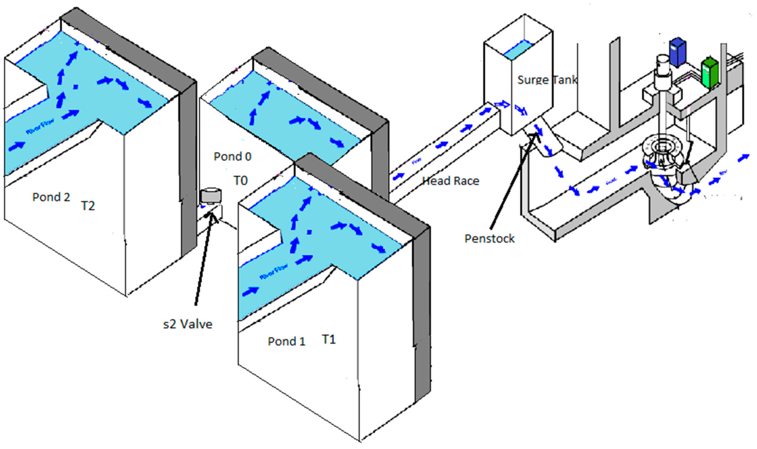
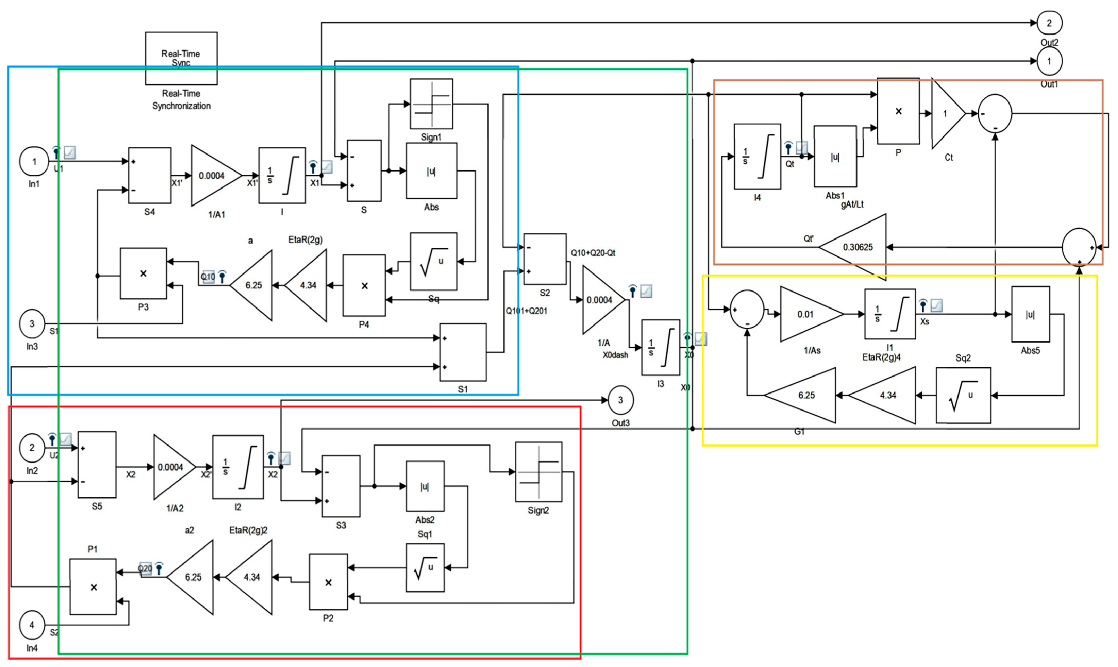
2. System Model

In a typical diverted ROR HPP, a weir or a short wall is placed on the riverbed to keep the water level in check. A weir varies from a dam in that it is designed to allow water to flow across it. The river is channeled, and the water is directed towards the head pond. The penstock or headrace is connected to the head pond (when a surge tank is present).

Figure 1 depicts the three head ponds or tanks of our run-of-river hydropower plant: $T_0$, $T_1$, and $T_2$. The ponds $T_1$ and $T_2$ are allowed to receive water from the river. Ponds $T_1$ and $T_2$ are connected to pond $T_0$ at the bottom. A surge tank connects the pond $T_0$ to the headrace tunnel, which leads to the penstock and turbine. The controllable valves s₁ and s₂ are located in the connecting tunnels between $T_1{T}_0$ and $T_2{T}_0$. In addition, remember that Figure 1 was adapted from [3,4] as a model with a single reservoir and then modified to fit our needs as a three-pound system. Another functional diagram of the system from the top view is given in Figure 2, which shows the plant’s interaction with the river.

While dealing with each part, the system is modeled as a series of equations. There are five equations because our hydraulic system comprises three ponds, a head race, and a surge tank. Ponds and tanks use the same mathematical model regarding water level change; the overall flow determines this into and out of the pond or tank. Because the headrace is a long tunnel, the water levels at each end determine the flow. The equations for the system are listed below.

As the main interest is in the water levels and flows, we formulate the equations of the ponds. The rate at which the water level changes in a pond or tank depends on the difference between inflows and outflows. The equation of such a pond is:

$$A\frac{d}{dt}x=inflow –outflow$$

(1)

A is the pond’s cross-sectional area, and x is the water level. The inflows and outflows between connected tanks are a function of the difference between the water levels.

$$flo{w}_{1\to 2}=f\left(x_1-x_2,a\right)$$

(2)

where $x_1$, $x_2$ are the two ponds’ water levels, and $a$ is the duct’s cross-sectional area or opening between the two ponds. For ponds 1 and 2, the inflow from the river and the outflow are to pond 0. We assume that the inflow from the river is completely controllable.

The outflow to pond 0 depends on the levels of ponds 1 and 0 and the duct’s cross-sectional area between them. Therefore, by combining Equations (1) and (2) and expanding them, the equations for ponds 1 and 2 are obtained.

Pond 1 has the following equation:

$$\frac{d}{dt}{x}_1=-\frac{ȵa}{A}{s}_1\sqrt{2g\left|x_1-x_0\right|}sgn\left(x_1-x_0\right)+\frac{U_1}{A}$$

(3)

Pond 2 has the following equation:

$$\frac{d}{dt}{x}_2=-\frac{ȵa}{A}{s}_2\sqrt{2g\left|x_2-x_0\right|}sgn\left(x_2-x_0\right)+\frac{U_2}{A}$$

(4)

where $sgn\left(z\right)$ is defined as:

$$sgn\left(z\right)=\left\{\begin{array}{cc}1& z>0\\ 0& z=0\\ -1& z<0\end{array}\right.$$

(5)

and $\left|z\right|$ is defined as:

$$\left|z\right|=\left\{\begin{array}{cc}z& z\ge 0\\ -z& z<0\end{array}\right.$$

(6)

The signum function included in the flow expression for the above equations determines the direction of water flow. In addition, note that the equations of pond 1 and 2 outflows are intentionally written before the inflow to be in line with the classical representation of a system, as we assume we have control over the inflow of water. For pond 0, it has three inflows and outflows. Water flows from ponds 1 and 2 and flows out to the headrace. So, Pond 0 has the following equation:

$$\frac{d}{dt}{x}_0=\frac{ȵa}{A}{\displaystyle ⎡}{s}_1\sqrt{2g\left|x_1-x_0\right|}sgn\left(x_1-x_0\right)+s_2\sqrt{2g\left|x_2-x_0\right|}sgn\left(x_2-x_0\right){\displaystyle ⎤}-\frac{Q_t}{A}$$

(7)

In the above Equations (3), (4) and (7), the control variables are $s_1, s_2$ and $U_1, U_2$, where $U_1, U_2,$ are the controllable inflow of water in ponds 1 and 2 in cubic meters per second, while $s_1 s_2$ are the dimensionless controllable valves between Pond 1 and 0 and Pond 2 and 0, respectively. While $ȵ$ is the discharge or flow rate coefficient and is the ratio of actual flow and theoretical flow or discharge [43]. Theoretically and unimplemented, the system’s value is arbitrarily taken as 0.98 to model the friction losses. The water levels, in meters, are $x_{1,}{x}_2,x_0$; $Q_t$ is the rate of flow through the headrace in cubic meters per second; A is the area of the ponds in square meters; a is the cross-sectional areas of the headrace and connecting tunnels between ponds 1 and 0, and 2 and 0, in square meters; and finally, $g$ is the gravitational acceleration in meters per square seconds.

The equation of headrace is derived from the flow in a tube. For the flow of water in a closed channel between two water reservoirs, 1 and 2 are given by:

$$\frac{L}{ag}\frac{d}{dt}Q=x_1-x_2-frictionlosses$$

(8)

where $L$ and $a$ are the lengths and cross-sectional area of the closed channel in meters and square meters, respectively, and g is the gravitational constant, and $x_{1,}{x}_2$ are the levels in reservoirs 1 and 2, respectively. Therefore, the closed channel’s flow direction changes as the two reservoirs’ water level changes. So the equation for the headrace is:

$$\frac{d}{dt}{Q}_t=\frac{g{A}_t}{L_t}\left(x_0-x_s\right)-C_t{Q}_t\left|Q_t\right|$$

(9)

The inflow is from the headrace for the surge tank, while the outflow is to the turbine penstock. As stated earlier, we do not include the turbine and penstock in this work, so the surge tank equation is:

$$\frac{d}{dt}{x}_s=\frac{Q_t}{A_s}-\frac{ȵa}{A_s}\sqrt{2g{x}_s}$$

(10)

These five Equations (3), (4), (7), (9) and (10) can be put together to form a nonlinear system model:

$$\frac{d}{dt}\overrightarrow{x}=\overrightarrow{f}\left(\overrightarrow{x},\overrightarrow{u}\right)$$

(11)

The state variables are located as follows:

$$\overrightarrow{x}={\left[x_{1 }{x}_2{x}_{0 }{Q}_t{x}_s\right]}^T$$

(12)

And the control variables are located as follows:

$$\overrightarrow{u}={\left[U_1,U_2,s_1,s_2\right]}^T$$

(13)

The outputs are $x_1$, $x_2$, and $x_0$. The output equation is:

$$\overrightarrow{y}=C\overrightarrow{x}$$

(14)

where C is defined as:

$$C=\left[\begin{array}{ccccc}1& 0& 0& 0& 0\\ 0& 1& 0& 0& 0\\ 0& 0& 1& 0& 0\\ 0& 0& 0& 0& 0\\ 0& 0& 0& 0& 0\end{array}\right]$$

(15)

where $U_1$, $U_2$ are the controlled water flow rates into the ponds $P_1$ and $P_2$ and $s_1$, $s_2$ are the valves between the ponds $P_1$, $P_0$ and $P_2$, $P_0$ respectively. The valves $s_1$, $s_2$ can be adjusted from 0 to 1 while $U_1$, $U_2$ can be adjusted from 0 to $U_{max}$. Figure 3 shows the Simulink implementation of the system model (Equation (11)). The Simulink model used to simulate the system is constructed by individually implementing all five system equations. The equation for pond 1 T1 is implemented in the top left corner of the figure, enclosed by a blue square. Similarly, the equation of pond 2 is implemented in the bottom left of the figure, enclosed by a red square. As the equation of pond 0 has the terms of both equations of pond 1 and 2, it is implemented using the elements of the other two equations on the center of the figure, enclosed by a green rectangle. Note that it encloses parts of the blue and red rectangles. Similarly, the equation of the headrace enclosed by brown is on the top right side of the figure, and the equation of the sure tank is implemented in the center right of the figure enclosed in yellow.

3. Control Design

The three-pound system must maintain the water level in ponds at a predefined level. Compared to a single pond, this system is distinguished from the conventional R.O.R. system by its three-pond mechanism. This working model analyses the water dynamics of the system. This work does not include a turbine, whereas the water level regulation of the system is performed by a Fuzzy Inference Engine (F.I.E.). Fuzzy Inference Engine or fuzzy control is used due to its flexibility in maintaining the water levels for the three ponds at different levels. Another advantage of using a fuzzy controller is its higher speed (especially in terms of settling time for this case, as the Fuzzy Controller settles as soon as the desired level is achieved and has no overshoot) and accuracy than traditional P.I.D. controllers. The advantage of the fuzzy controller over PID in terms of having no overshoot and earlier settling time can be seen in Figure 10 in [44] (preprint of this manuscript).

Fuzzy Control

The control scheme is slightly unlike the traditional one, using the system output states and the errors.

$U_1$,$U_2$, $s_1$, and $s_2$ are control variables in the system defined in (Equation (11)) whereas $x_0$, $x_1$, and $x_2$ out of five states need to track their desired levels. The system control uses two fuzzy inference engines and subtractors. The Simulink-based elaborate control scheme is given in Figure 4.

The subtractor calculates the difference between current and intended state values. It allows changing required levels without creating new rules for F.I.S.

Subtractors generate pond errors $E_0$, $E_1$, and $E_2$, and depending on errors being positive, negative, or zero, F.I.S. makes decisions. F.I.S. is the most crucial component of the control system, constituted by IF-THEN rules. For example, if a system has two inputs and one output, the rules are formed:

$$Rule 1: IF x_{1 }is A_{1 }^1 and x_{2 }is A_{2 }^{1}THEN y is B^1$$

(16)

A complete rule set comprises all possible input memberships’ combinations. For example, if a two-input system has both inputs with three memberships, then all the possible memberships combinations are $3\times 3$ or $3^2=9$ rules. The outputs can have a number of memberships, the same as the number of rules or less.

Because each rule has six inputs and four outputs, the complete rule base for this system requires 3⁶ = 729 rules for effective system control. Furthermore, each input has three levels, and the output has five. This causes increased mathematical overhead and slowing of simulation. By replacing one fuzzy system with two parallel ones, the problem is avoided. Fuzzy System 1 ($F{S}_1$) regulates $U_1$ and $s_1$ by dealing with Pond 0 and Pond 1, whereas Fuzzy System 2 ($F{S}_2$) regulates $U_2$ and $s_2$ by dealing with Pond 0 and Pond 2. So each Fuzzy system has four inputs and two outputs. The number of rules is now reduced to $3^4=81$ for each system. Maintaining the ponds’ water levels at the desired level in the three-pond system is required. Due to the simulation hardware limitations, the membership functions were chosen to be triangular or trapezoidal due to their simplicity. As the results show, even the simplistic membership functions yielded acceptable results. As the membership functions are between 0 and 1 Gaussian, exponential or sigmoid functions could have represented them, they would have made our already slow hardware even slower, or made the simulation intractable. Therefore more simplistic triangular and trapezoidal functions were used. The inputs of F.I.E. are current water levels and error values, whereas the value positions and the inflows are outputs. F.I.S. regulates (maintains, increases, or decreases) the levels of ponds by varying the values of inflows $U_1$, $U_2$ and valves’ positions $s_1$, $s_2$. The values can be varied from 0 to some maximum positive value for inflows and from 0 to 1 for valve position. The positive error can be reduced by stopping the inflow and depending on the outflow to lower the level. In contrast, managing negative error requires the inflows to be greater than outflows. The zero error is maintained by equaling the outflows and inflows. The valves are specifically used when the ponds need to be set at different levels. A simplified pseudo-code for FS1 is given in Algorithm 1. As stated before, the control variables U1 and s1 control the levels of Pond 1 and 0.

Algorithm 1. Simplified pseudo code for Fuzzy System 1 controlling levels of Pond 1 and 0.

1: Start 2:   Take required pond levels 3:Check level of pond 1 and 0 4:   IF (Pond levels are lower than required level) Increase the value of inflow U1 and Hold valve S1 5: ELSE IF (The pond level is greater the required level) 6:Stop the inflow U1 and increase the position of S1 7:      ELSE IF (The ponds levels are same as required level) 8:      Decreased U1 and S1 until inflow and outflow is balanced 9:      Hold the position of U1 and S1 10:    END IF 11:    Repeat steps 1 to 10 12:    Stop

Trapezoidal membership functions are assigned to heights with HIGH, MEDIUM, and LOW water levels. Trapezoidal membership functions are also assigned to POSITIVE and NEGATIVE errors, whereas ZERO is assigned with a triangular membership function. The membership functions used are self-explanatory, and the ZERO membership function is meant for near-zero errors. Each output has five levels from 0 to 4, where Level 0’ stops and level ‘4’ is maximum or full throttle. Level ‘0’ is not defined for ‘U’, and valves s_i(for i = 1, 2) have impulse membership functions at zero or maximum. Membership functions assigned to all outputs are trapezoidal. Figure 5 shows the input and output membership functions.

It is difficult and unnecessary to explain all the 81 rules for each fuzzy system, but a few examples are given to justify their basis.

(1) Considering zero initial conditions with a setdesired level, $x_1$ and $x_0$ are at LOW and $E_1$ and $E_0$ are negative, the output $U_1$ is required to have a high inflow rate $L_4$ and valve $s_1$ is to be set at open $V_4$. The conditions are given in the form of rules:

$$\begin{array}{c}IF E0 is NEGATIVE and E1 is NEGATIVE and X0 is LOW and X1 is LOW\\ THEN S1 is V4 and U1 is L4\end{array}$$

(17)

So, in the above Equation (17), the errors of ponds 0 and 1 are negativeand the water levels of ponds 1 and 0 low. This means both the ponds are empty or nearly empty, and the levels need to be increased fast, so both the inflow $U_1$ and $s_1$ are opened to full throttle.

(2) If both levels are at similarly high levels and both errors are zero, then it requires balancing of inflow and outflow rates, i.e., both $U_1$ and $s_1$ are set at positions to maintain the system in equilibrium. This is depicted in the form of the rule:

$$\begin{array}{c}IF E1 is ZERO and E0 is ZERO and X1 is HIGH and X0 is HIGH\\ THEN U1 is L1 and S1 is V1\end{array}$$

(18)

Here Equation (18) describes a situation in which both the errors are zero and the pond levels are high. As the errors are zero, we must keep and maintain the errors at zero level, so the inflows and outflows are balanced by keeping the inflow $U_1$ and valve $s_1$ at level 1 open.

(3) If both errors are zero, the level of $x_0$ is at mid-level and $x_1$ is high, then it requires balancing of inflow and outflow rates, i.e., both $U_1$ and $s_1$ are set at defined positions to maintain the system in equilibrium. This is depicted in the rule below:

$$\begin{array}{c}IF E0 is ZERO and E1 is ZERO and X0 is MEDIUM and X1 is HIGH \\ THEN U1 is L1 and S1 is V1\end{array}$$

(19)

The case in Equation (19) is same as Equation (18), except the pond 0 is at mid level. So, to maintain the current levels of inflow, $U_1$ and valve positions are kept the same as in Equation (18).

(4) If there is zero error for $E_0$ and positive error for $E_1$ but both levels are similarlyhigh; the priority is set for Pond 0. The valve $s_1$ is set to a defined position, and inflow is stopped at $L_0$ to maintain Pond 0 in equilibrium, Pond 1 is reduced. This is depicted in the rule below:

$$\begin{array}{c}IF E0 is ZERO and E1 is POSITIVE and X0 is HIGH and X1 is HIGH \\ THEN S1 is V1 and U1 is L0\end{array}$$

(20)

In this case of Equation (20), pond 0 is at the desired level, but pond 1 is greater than the desired level, while the levels of both ponds are similarly high. Now, ideally, it is needed that both of the ponds should have zero error, but the head pond is more important. So, valve $s_1$ is kept at valve level 1 so that the inflow and outflow of pond 0 remain balanced, while the inflow $U_1$ is stopped so that pond 1 can slowly drain and reach the required level while pond 1 remains the same.

(5) If there is zero error for $E_1$ and positive error for $E_0$ and both the levels are similarlyhigh; then, the priority is set for pond 0. The valve $s_1$ is set to a defined position, and inflow is stopped at level 0 to get pond 0 drained to pond 1 and the headrace. This is given in the rule below:

$$\begin{array}{c}IF E0 is POSITIVE and E1 is ZERO and X0 is HIGH and X1 is HIGH \\ THEN S1 is V1and U1 is L0\end{array}$$

(21)

In this way, all rules for FS1 are designed, and the same are mirrored for FS2.

The fuzzy controller’s output can be expressed in a generalized manner as follows:

$$u\left(t\right)=\frac{{{\displaystyle \sum }}_{j=1}^{81}{\overline{u}}_j\left({{\displaystyle \prod }}_i^4{\mu }_{A_i^j}\left(k_i\right)\right)}{{{\displaystyle \sum }}_{j=1}^{81}\left({{\displaystyle \prod }}_i^4{\mu }_{A_i^j}\left(k_i\right)\right)}$$

(22)

where $u\left(t\right)$ is the controller’s output for $U_1$ or $s_1$, $k_i$ is the input value of $x_0,x_1,E_0$ and $E_2$. The linguistic variable for input that can be $NEG,ZERO,POS$ or $LOW, MED,HI$ is $A$, ${\mu }_A$ is the membership function of $A$ and ${\overline{u}}_j$ is the firing strength of $j^{th}$ fuzzy rule.

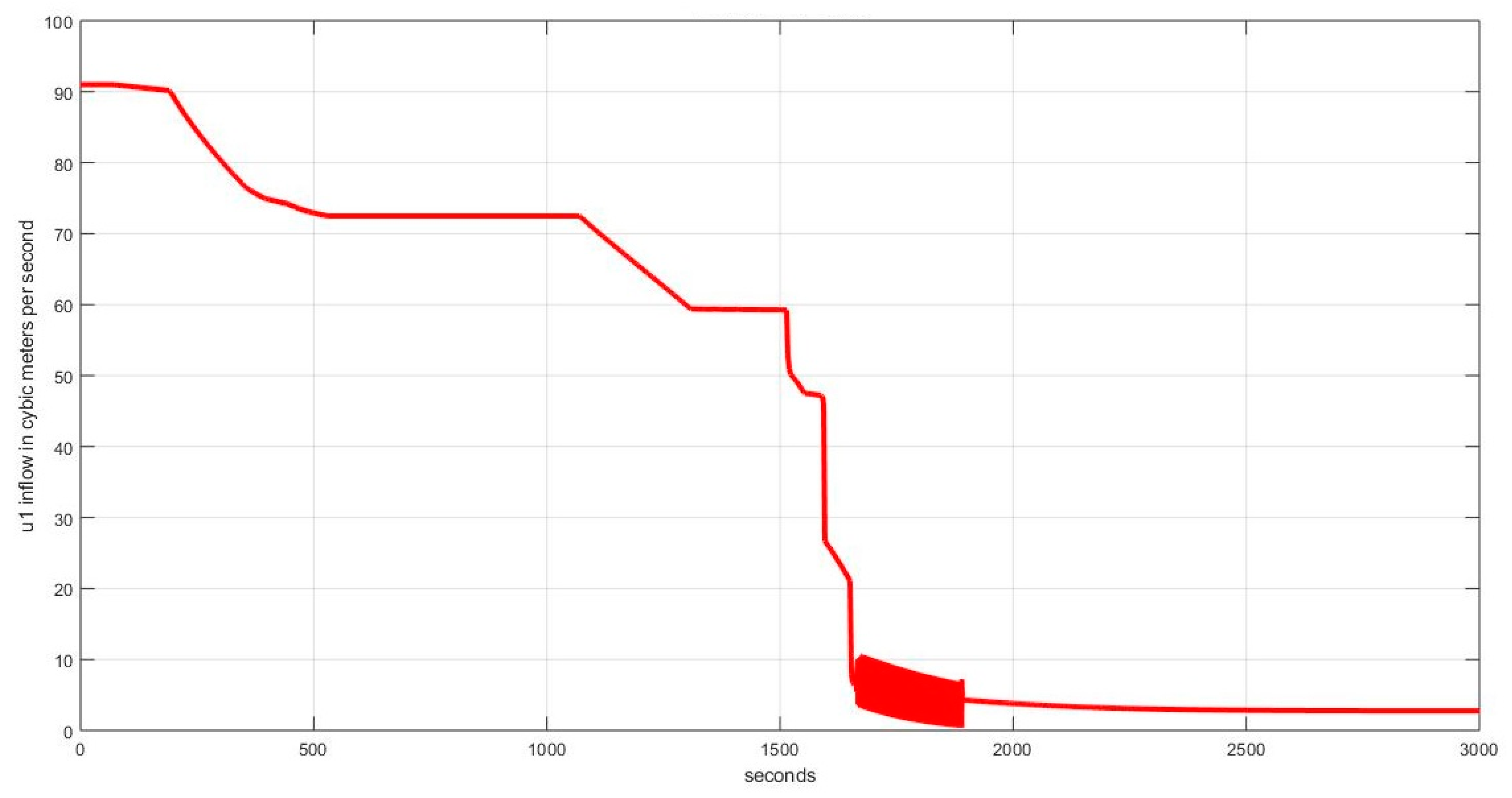
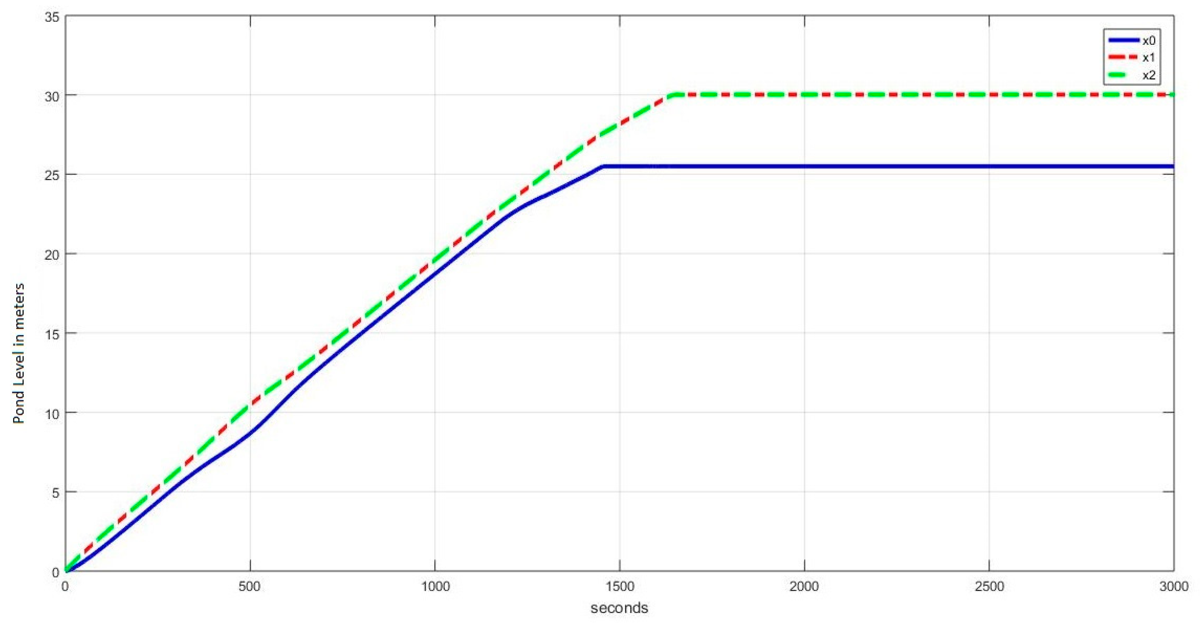
4. Results and Discussion

Extensive simulations analyze the proposed system in Simulink (MATLAB). The simulation is discretized by a fixed step size of 0.1 s, and Matlab/Simulink automatically chooses the solver. The results are compared with the conventional redirected run of the river hydropower plant. The proposed three-pond model is compared with a single-pond model with the same storage capacity as the other three tanks combined.

As a case study, the following values for the model parameters are used for simulations.

$H_0$ = $H_1$ = $H_2$ = Height of pond 0, 1, 2 = 35 m

$H_s$ = Height of Surge Tank = 15 m

$a$ = The area of the cross-section of the ducts between $T_1\&T_0$,$T_2\&T_0$ = $6.25 {\mathrm{m}}^2$

A = Area of the Ponds $T_0$,$T_1$,$T_2$ = $50\mathrm{m}\times 50\mathrm{m}$ = $2500{\mathrm{m}}^2$

$A_s$ = Area of Surge Tank. =$10 \mathrm{m}\times 10 \mathrm{m}$ = $100 {\mathrm{m}}^2$

$L_t$ = Length of headrace. = $200 \mathrm{m}$

$A_t$ = Cross-sectional area of head race =$6.25{\mathrm{m}}^2$

$U_{max}$ = The maximum controllable intake of water in ponds $T_1$ and $T_2$ = $100\raisebox{1ex}{${\mathrm{m}}^3$}\!\left/ \!\raisebox{-1ex}{$\mathrm{s}$}\right.$

Traditional System: Single-Pond Model

Proposed System: Three-Pond Model

T₀, T₁, T₂: pond 0, pond 1, pond 2

For a fair comparison of the three-pond model with the classic single-pond model, all parameters are the same, except that the pond area A of the traditional model is multiplied by3, and U_max is multiplied by 2. This preserves generality as well. Both systems’ levels are managed through fuzzy inference control. The assumptions taken for the simulation of the system are as follows:

The equations describe the system entirely, and the uncertainties of the model parameters do not exist.

All the control variables are completely controllable and have no transmission delay or actuator overload. Similarly, all the states are observable, with no sensor noise.

Any chattering or jittering of the control outputs does not affect the controller’s working.

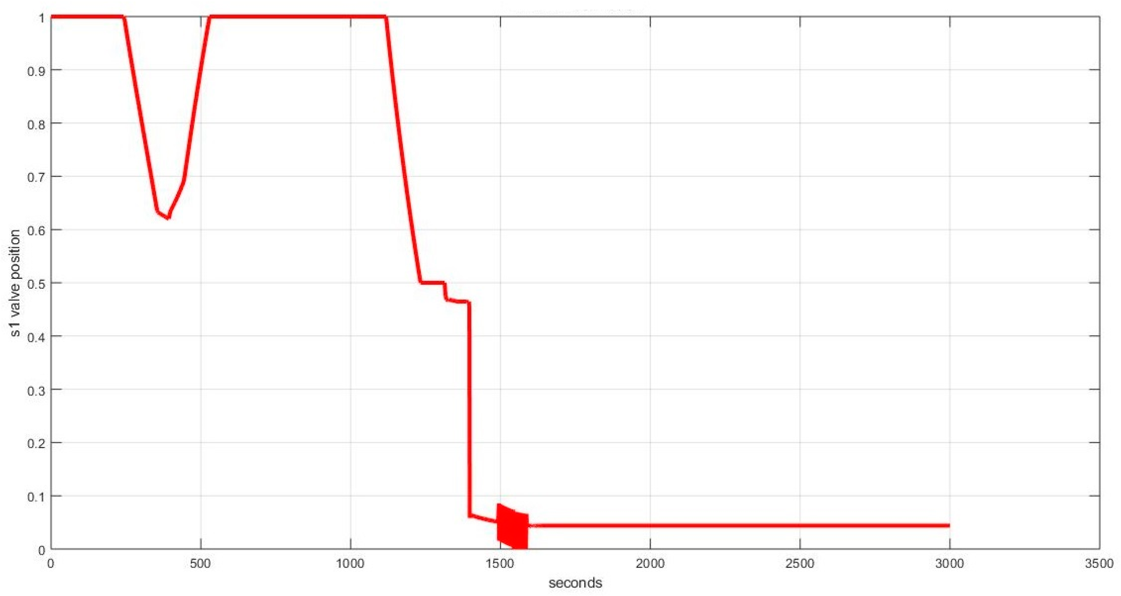
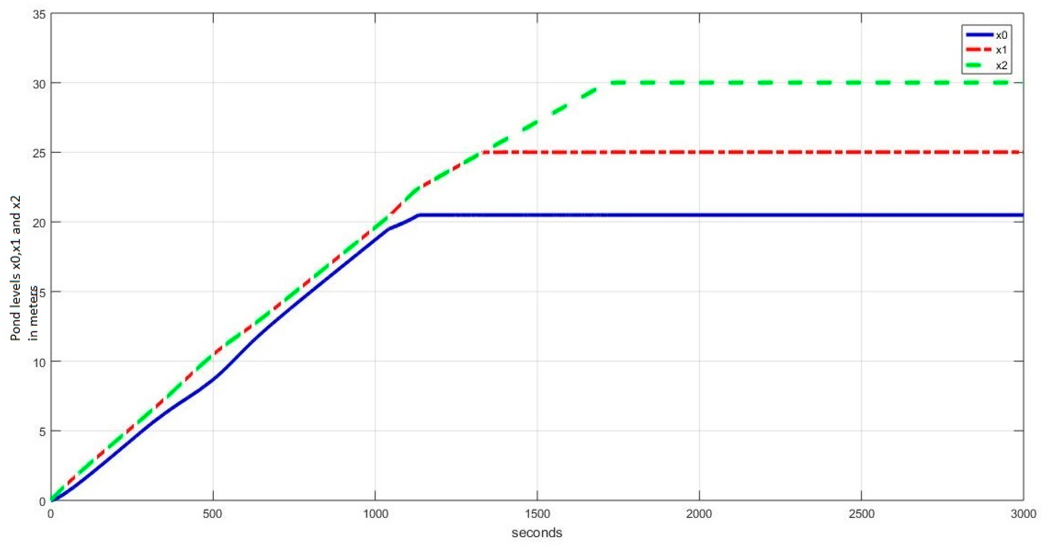
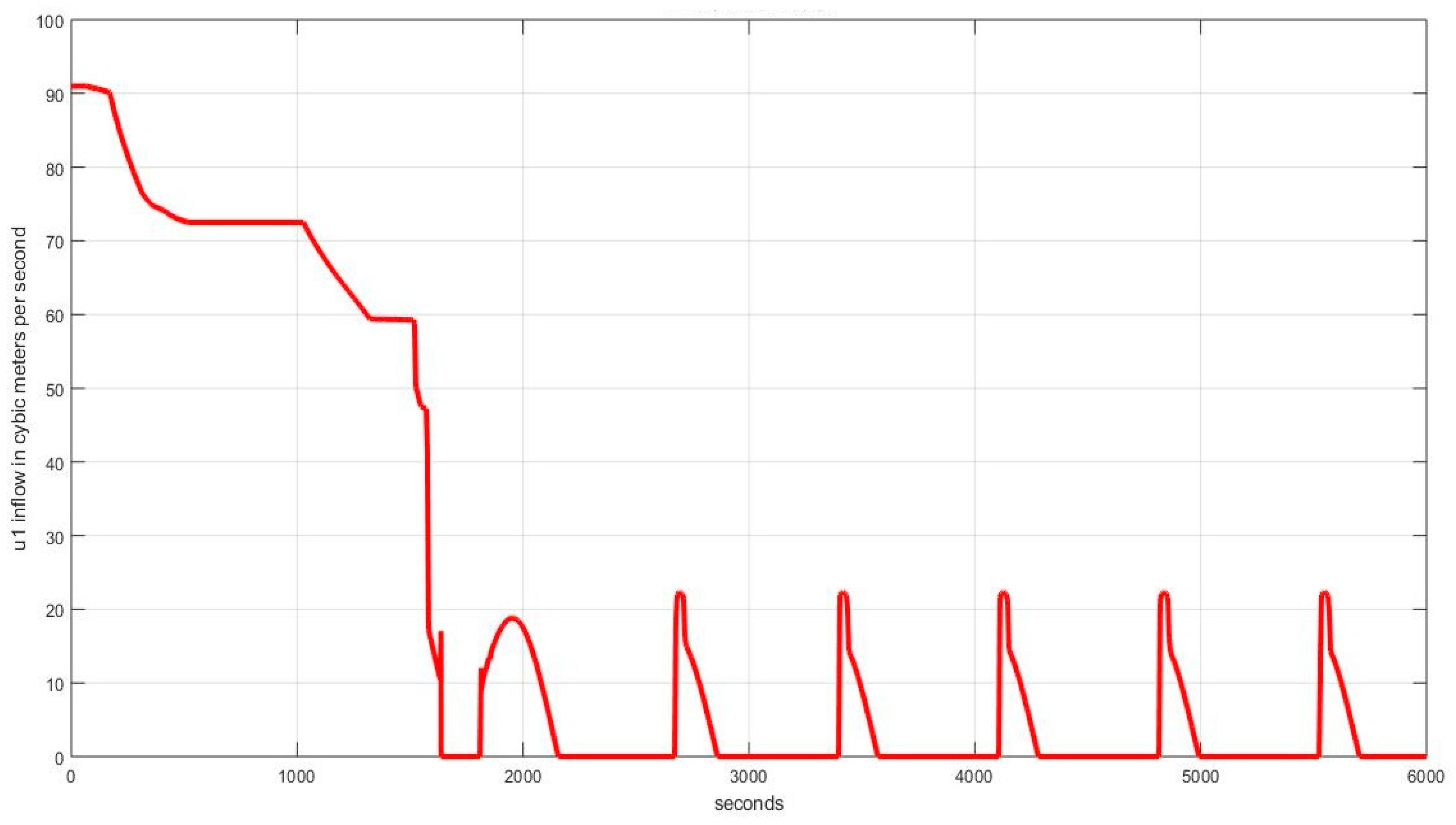
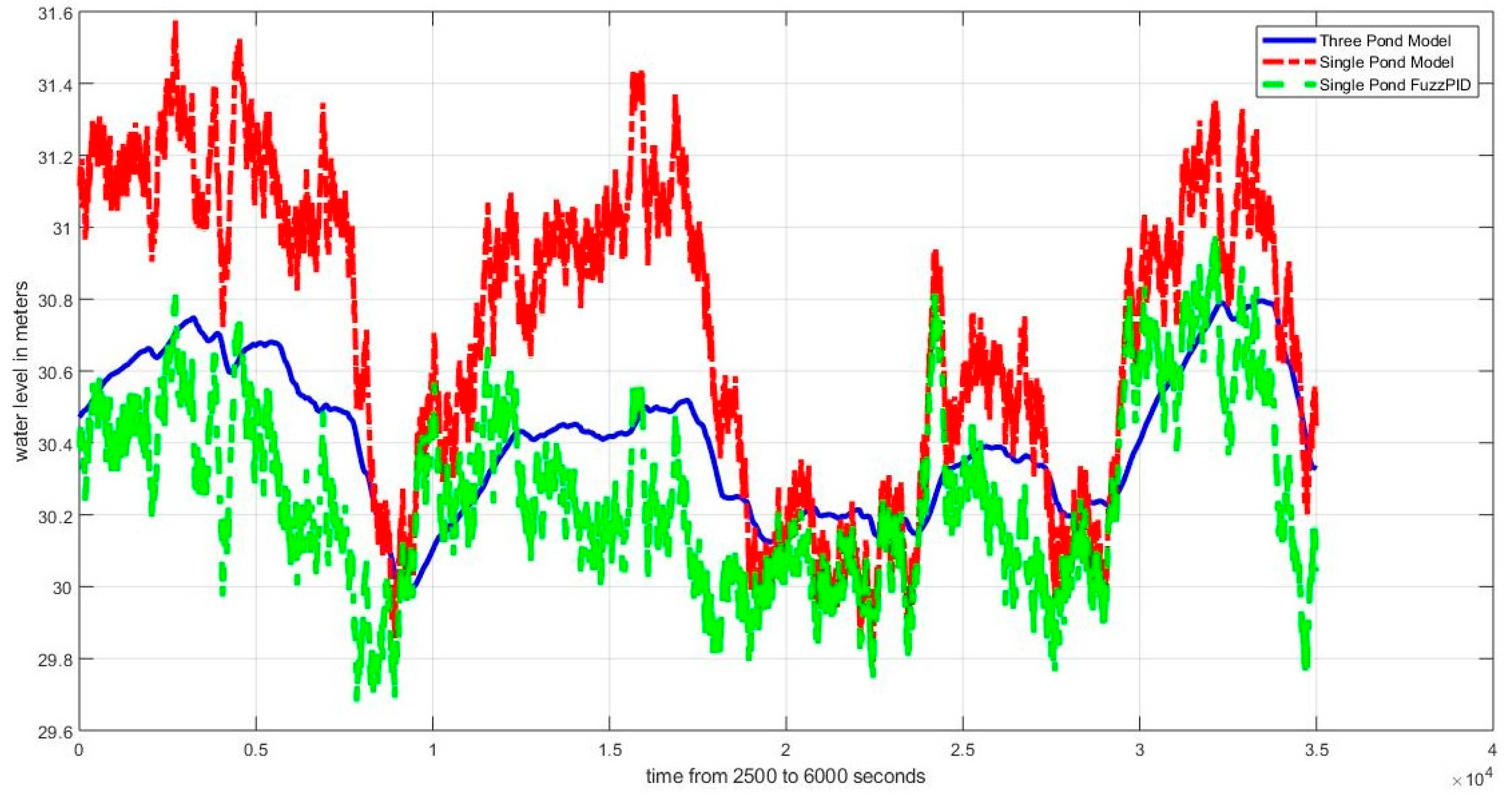
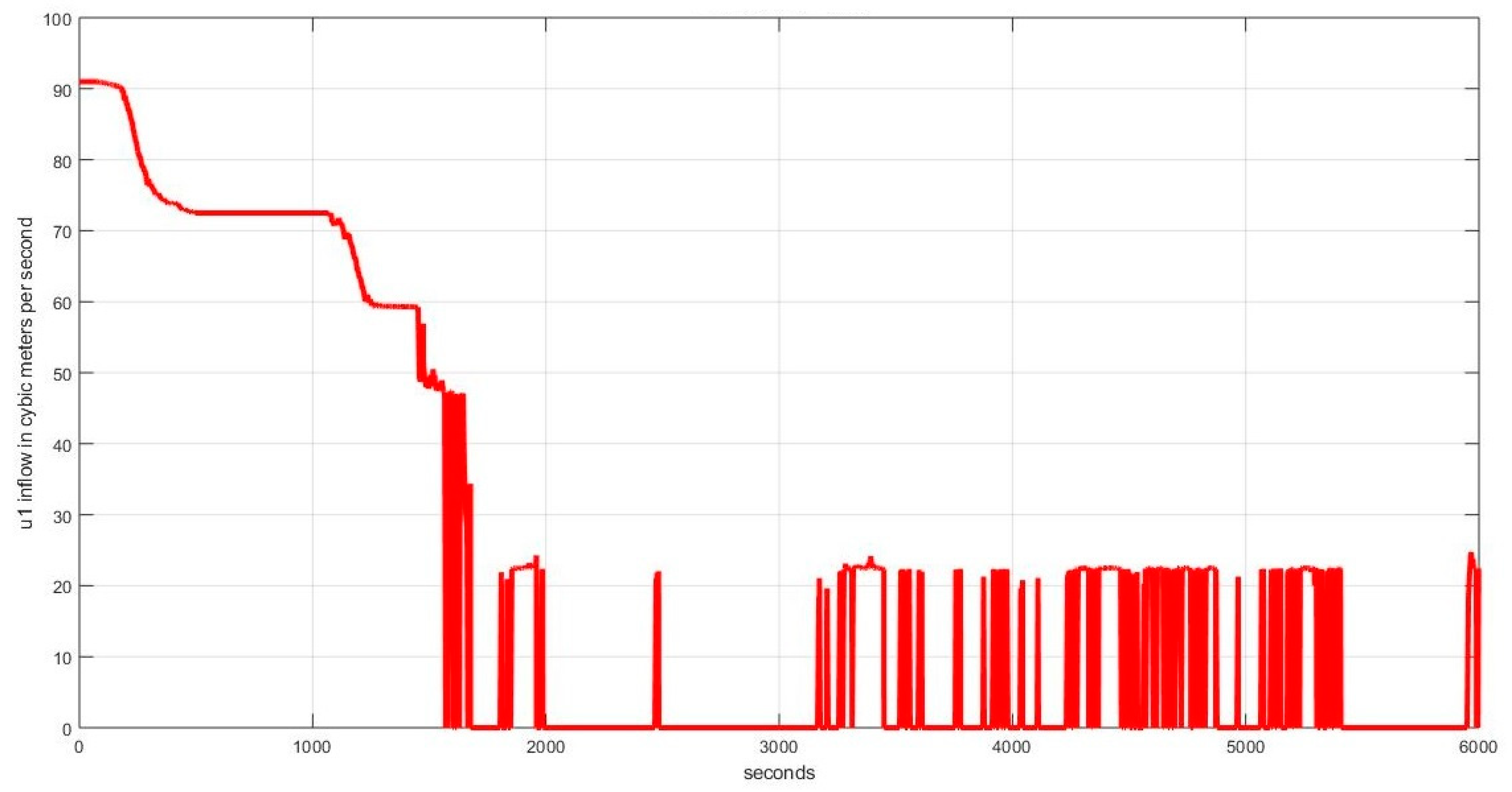
4.1. Level Regulation

This section discusses the results of the suggested F.I.S. for managing water levels in the proposed model. Three different instances are considered. The Case considers the water level in all three ponds to be the same. The second Case considers the water level in pond 0 to be less than in ponds 1 and 2, where ponds 1 and 2 have the same water level. The third Case considers the water levels in all three tanks to be different, such that pond 0 has the lowest water level, followed by pond 1, while pond 2 has the highest water level. Provided following are the results and their discussion.

4.1.1. Case I: ($T_0=30$, $T_1=30$, $T_2=30$)

In this case, a water level of 30 m is required for the three tanks. All three tanks are supposed to be empty initially. All states reach a steady state in almost 30 min. The inaccuracy in steady-state is 0.5 m. Ponds $T_1$ and $T_2$ take different times, as compared to a pond $T_0$, to reach a steady state. They take 27 min to rise to a steady state whereas $T_0$ takes 30 min. Figure 6 shows a graphical representation of these results. The findings suggest that the proposed scheme can maintain the desired water levels. A balance between water inflow and outflow is maintained when the system reaches a steady state. The graphical representation of the control variables U1 and s1 are shown in Figure 7 and Figure 8, respectively. The reason for showing the $U_1$ and $s_1$ variables in different figures is their vast scale difference. As shown in Figure 6, the magnitude of U1 decreases with the increase in the water level reaching the desired level until the current level is just near the required level. At this point, the $U_1$ switches between Level 1 and Level 2 for a while till the equilibrium is reached and the $U_1$ is left at the level 1. Similar is the case with the s1 control variable. The spike in s1 appears a little before x0 reaches the desired level because the level of $x_0$ and $x_1$ (or $x_2$) is increased before all three ponds settle at the required level.

4.1.2. Case II: ($T_0=25$, $T_1=30$, $T_2=30$)

Here, a water level of 25 m is desired for pond 0, whereas 30 m is desired for pond 1. The system takes 30 min to reach desired water levels in ponds 1 and 2. It takes 24 min to reach the desired level in pond 0; for pond 0, the desired water is 25 min, and the steady-state error is 0.5 m. Figure 9 shows these results graphically, where the blue line represents the water level of pond 0, and the dotted green and red lines represent the water levels in ponds 1 and 2, respectively. The control variables U1 and s1 are shown in Figure 10 and Figure 11, respectively. The behavior of U1 and s1 is similar to the previous case with slight differences as the required levels and time required to reach the required levels are changed.

4.1.3. Case III: ($T_0=20$, $T_1=25$, $T_2=30$)

In this case, the water levels of ponds 0, 1, and 2 are 20, 25, and 30 m, respectively. T₀ reaches its desired level in about 18 min, T₁ in 22 min, and T₂ in 27 min. The system takes less than 30 min to reach a steady state. Where a steady-state error of 0.5 m is shown by T₀, an almost negligible steady-state error is shown by T₁ and T₂. Figure 12 shows these results graphically. As the behavior of the control variables is the same as in the previous two cases, they are not shown.

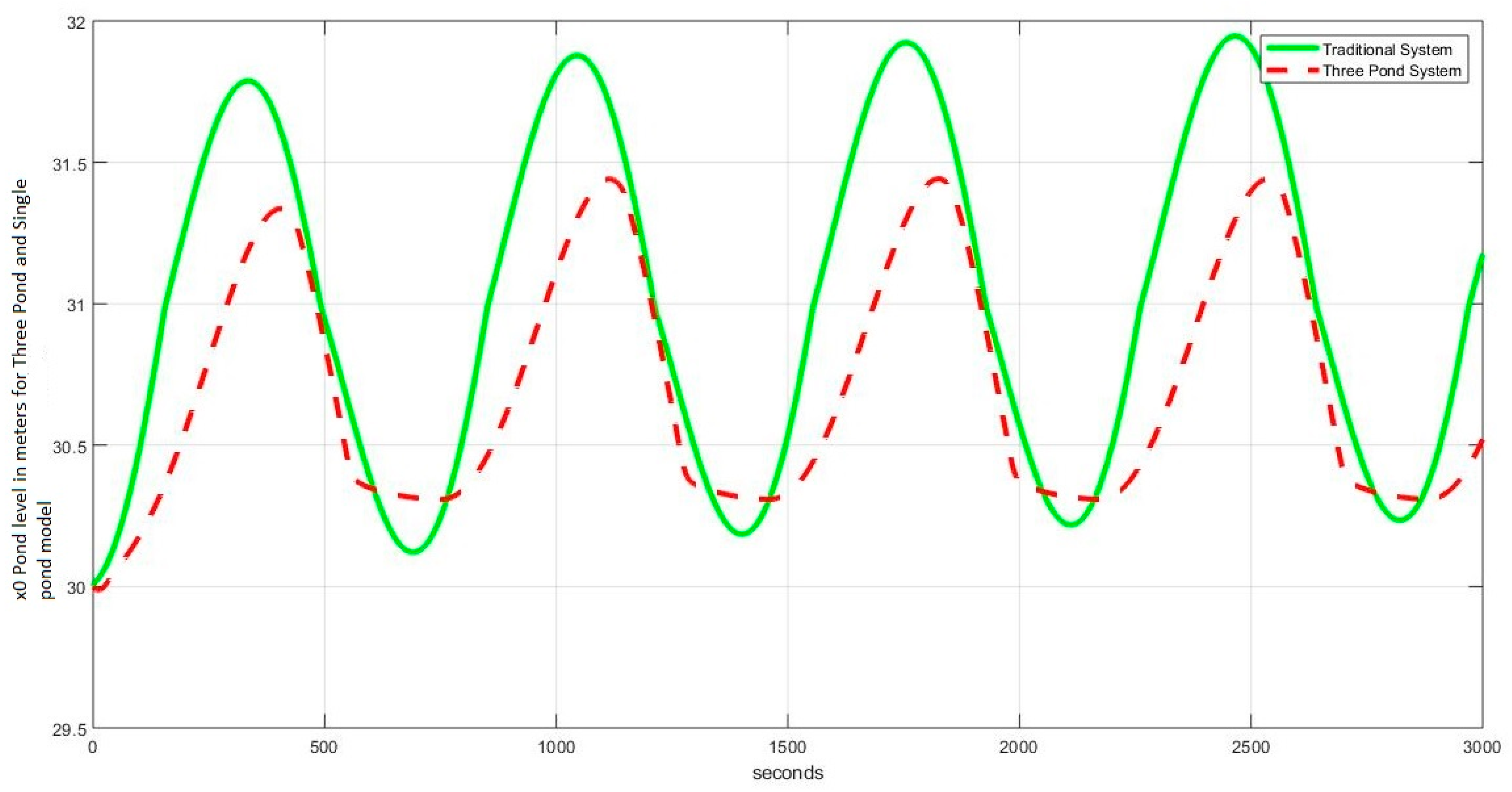
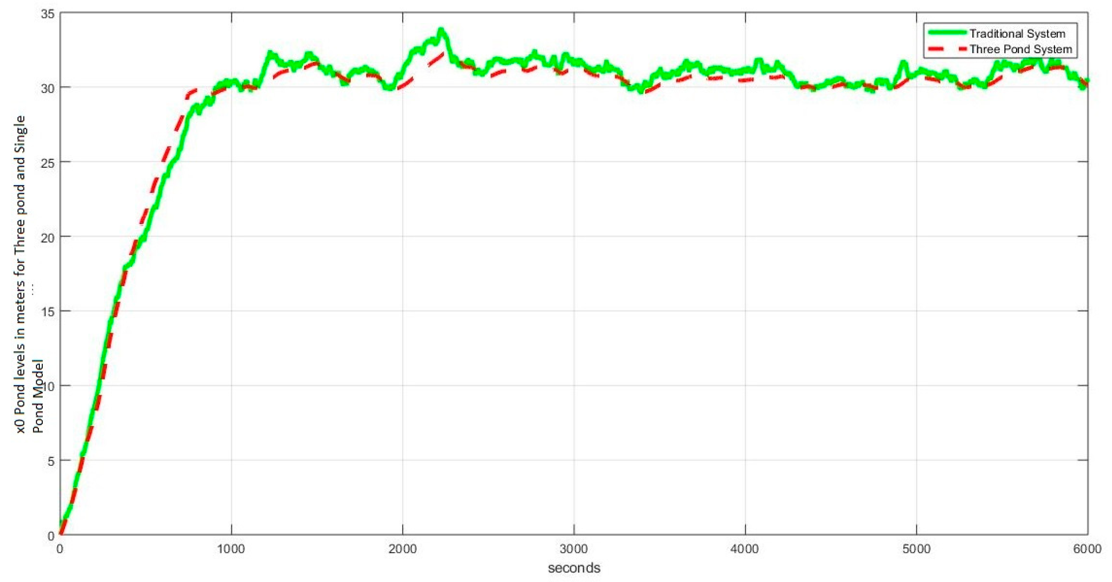
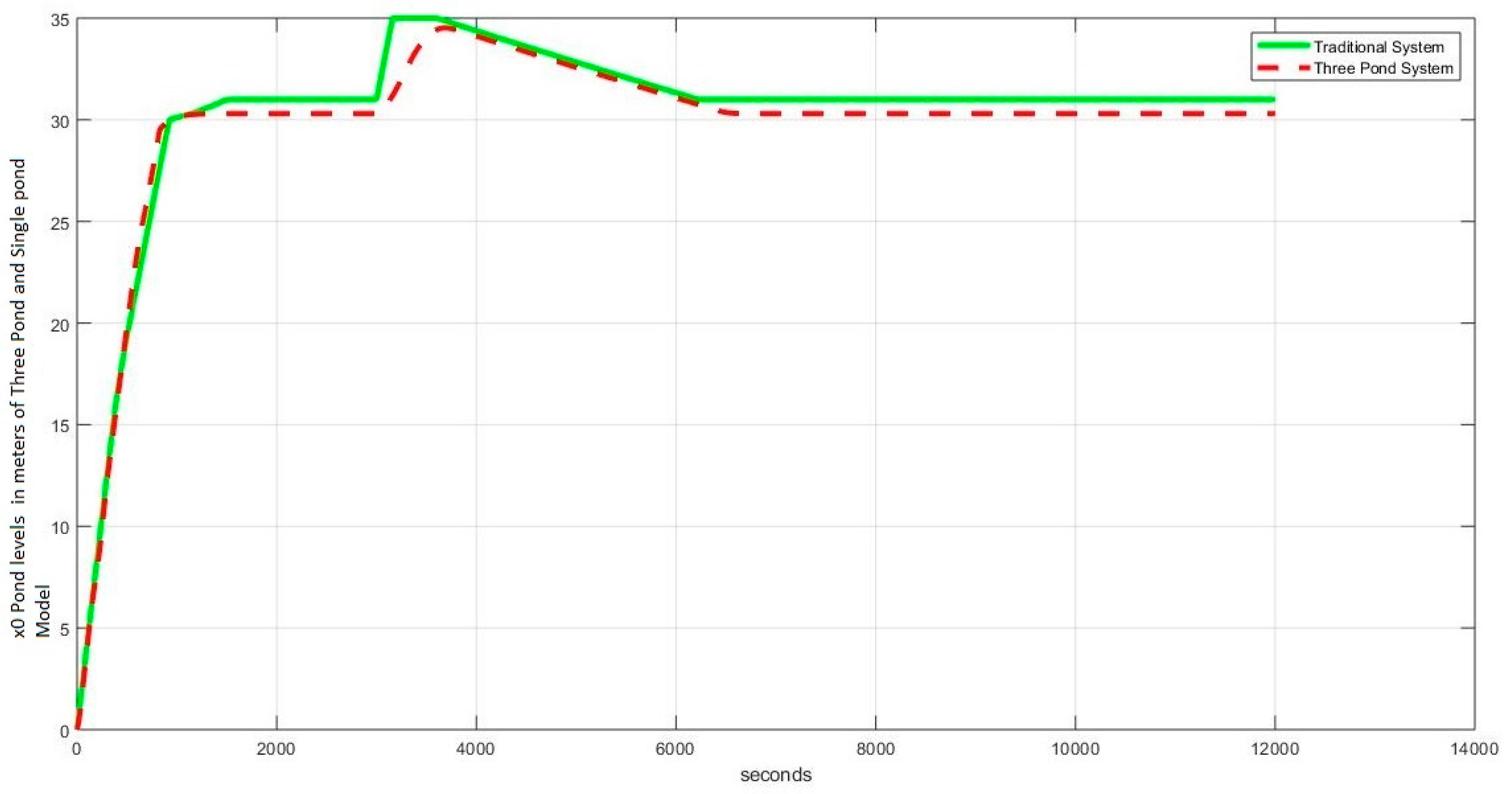
4.2. Robustness Analysis

This section provides analysis and discussion regarding the robustness of the proposed model of ROR HPP controlled with F.I.S. Simulations are done to check the system’s response for four disturbances: white noise, sinusoidal, positive and negative, and sudden surge. The proposed system is compared with a traditional system with fuzzy control and then with a traditional system with fuzzy PID hybrid control. The traditional single-pond systems are controlled by fuzzy control like the proposed system in the first case and with Fuzzy PID hybrid control in the second case. Next, these disturbances are utilized to check the response when the system has half capacity. However, the proposed system is tested only against traditional single-pond systems with fuzzy control. The system’s capacity may be halved by decreasing the depth of the pond or its area to half of the original. We have reduced the area instead of depth because reducing the depth/Height of the pond necessitates redesigning or modifying the fuzzy inference system. The different cases are tested for the system at zero initial conditions (empty ponds) and initial steady-state conditions.

4.2.1. Case Ia: Sinusoidal Disturbance (Three-Pond System vs. Single-Pond System)

For a fair comparison between the systems, the parameters of the three-pond system are matched with that of the traditional single-pond system. Comparison against disturbances is made because the two systems expectedly take the same time to reach desired steady states. An additive sinusoidal disturbance $d=a.sin\left(wt\right)$ with the controllable inflow of water is added to the system $U=\left[U_1,U_2\right]$. Differences in behaviour begin to appear when the three systems approach steady states. During transitory situations, all systems normally perform, as shown in Figure 13. In steady-state, the proposed three-pond system efficiently suppresses the disturbances’ effects, while the traditional single-pond system does not suppress these effects so efficiently. The FuzzyPID has some degree of improvement over the Fuzzy single-pond system, but the proposed three-pond system is markedly better at disturbance suppression. In Figure 14, the steady states of the systems are shown from 3000 s to 6000 s (from 50 min to 1 h 40 min). By analyzing the steady state graphs and data, we find out that the variation in the traditional single-pond system is 0.7 m while the peak variation in pond 0 of the proposed system is 0.3 m, so the proposed system suppresses nearly 57% of the sinusoidal disturbance as compared to the single-pond model. This demonstrates the effectiveness and robustness of the FIS-regulated proposed model against sinusoidal disturbances. Figure 15 and Figure 16 show the behavior of the control variables U1 and s1 when facing a sinusoidal disturbance. The behaviors of U1 and s1 are the same as in Figure 7 and Figure 8 in transitional states, but change considerably as the system reaches a steady state. In a steady state, U1 drops to 0 whenever there is a positive sinusoidal half cycle but is turned on during the negative half cycle. On the other hand, the magnitude of s1 is lowered again and again slightly to keep the level of pond 0 near the desired level.

4.2.2. Case Ib: Sinusoidal Disturbance (Three-Pond System vs. Single-Pond System, Half Capacity)

The simulations described above are repeated for the half-capacity case with some minor modifications. With the system capacity being half, the system rise time is faster. As in the previous case, the effects of disturbance are not so pronounced in the transient states, and difference in behaviour appears only when the systems approach steady states. The responses of the two systems are shown in the figures below. Figure 17 and Figure 18 show that the proposed model efficiently mitigates the effects of the disturbances while they are much more pronounced for the traditional single-pond system. The control actions are the same as in the previous case, so they are not discussed here again.

4.2.3. Case IIa: White Noise Disturbance (Three-Pond System vs. Single-Pond System)

In the previous case, we added sinusoidal disturbances to the systems. Here, we add random additive white noise. Identical amounts of noise are added to two systems. In the case of three-pond systems, the noise is between ponds T₁ and T₂. Contrary to the Case of sinusoidal disturbances, the effects of disturbances are also visible in transient states. However, the proposed system suppresses the effects of the high-frequency components of the disturbance. The Fuzzy PID control also has some degree of disturbance suppression for the single-pond model, but the proposed three-pond model is markedly better. Figure 19 and Figure 20 show this disturbance’s effects on all three systems graphically. Figure 19 shows the steady states from 2500 s to 6000 s. Analyzing the graphs and data, we see that the maximum deviation for the traditional system is around 1.6 m, in addition to being affected by high-frequency components.

In comparison, pond 0 of the 3 pond system has 0.9 m of variation and suppresses the disturbance’s higher frequency components. Overall, the proposed system suppresses nearly 44% of the disturbances compared to the traditional system. As in the previous case, the control variable behaves normally duringthe transient phase, but U1 needs to keep switching between L1 on and L0 off as depicted in Figure 21, while s1 is also observed behavingthe same way but with lesser frequency as shown in Figure 22.

4.2.4. Case IIb: White Noise Disturbance (Three-Pond System vs. Single-Pond System, Half Capacity Case)

Here the two systems are supposed to be operating at half capacities. The effects of the disturbances are visible in the transient and steady states. However, these effects are much less in the Case of the three-pond system. The high-frequency components of the disturbance are also suppressed by the three-pond system. The response of the two systems is graphically given in Figure 23 and Figure 24.

4.2.5. Case IIIa Positive Surge Disturbance (Three-Pond System vs. Single-Pond System)

Equal amounts of positive surges of some predetermined durations are added to the system when they reach steady states, and their response is noted. In this case, it is observed that the proposed model suppresses the positive surge’s effects efficiently. In addition, the traditional system is observed to have been overflown for some time for both controls. However, the proposed system does not overflow. Figure 25 and Figure 26 show the behaviors of the two systems graphically. Analyzing the graphs, we see that the traditional system has a sharper surge which also causes the pond to overflow for a few minutes, while the proposed system has a gentler surge and does not overflow the pond. As the pond of the traditional system overflows, it is not easy to quantify the disturbance suppression of the proposed system. Control variable U1 closes off completely (Figure 27) as soon as the surge appears and opens to the L1 level after its effects have dissipated. At the same time, the control variable s1 behaves normally (Figure 28) in transition and steady states.

4.2.6. Case IIIb Positive Surge (Three-Pond System vs. Single-Pond System (Half Capacity)

The exact process is carried out in this instance for the half-capacity case. When the systems reach steady states, positive surges are added to them. More severity is observed in the two systems’behaviour compared to the previous Case when the plans were operating at full capacity. The proposed model can somewhat suppress the positive surge’s detrimental effects. In this case, the traditional system overflows, and the overflow is more than in the previous Case. The proposed model does not overflow. Figure 29 and Figure 30 graphically show these results.

4.2.7. Case IVa Negative Surge (Three-Pond System vs. Single-Pond System)

This experiment is similar to the previous Case, but a negative surge is provided to the system when they reach steady states instead of a positive surge. The effects of the negative surge in the proposed system are much less than that in the traditional system with both controls. The traditional system shows a sharp dip and then smooths out. Figure 31 and Figure 32 graphically show the behaviors of the two systems. The graphs and data show that the traditional system dips about 1.9 m for the negative surge. In comparison, the proposed system dips only 0.8 m for the same disturbance, thus suppressing nearly 59% of the disturbance. The control variables (u1,s1), as shown in Figure 33 and Figure 34, behave normally, but both inflow U1 and valve s1 open to compensate for the effects of the negative disturbance during its presence.

4.2.8. Case IVb Negative Surge (Three-Pond System vs. Single-Pond System, Half Capacity)

This time, a negative surge is provided to the two systems operating at half capacity on reaching steady states. The effects of the negative surge are observed to be the same, but the severity is more than in the previous Case. The system responses are graphically shown in Figure 35 and Figure 36.

4.3. Observations

As shown in the above test cases, the proposed three-pond model not only suppresses the disturbances about 40% to 60% for most cases, it also smoothes outthe transitions resulting from disturbances. Even when hybrid Fuzzy PID improves the control of the traditional system, the proposed three-pond system is inherently better at smoothing out high frequency disturbances and suppressing disturbances. This means after a turbine or a power generator is installed, this system not only has the potential to provide power more stably, but the power controllers at the distribution end will also be less stressed in trying to attenuate disturbances.

5. Conclusions

This work used a three-pond model in a run-of-river hydropower plant to reduce its dependency on the river’s seasonal flows and make it robust against disturbances. Because the three-pond hydraulic model is highly nonlinear, the fuzzy inference system is used as a control scheme. The demand was stabilizing pond water levels, resulting in long-term energy generation. The results showed that the three-pond model outperformed the standard single-pond model in maintaining water levels. The system has also been tested against four different disturbances, i.e., sinusoidal disturbance, white noise disturbance, and positive and negative disturbance. The system shows better disturbance suppression as it is more robust in frequency and overshoot. This paper uses the three-pond model for a hydropower plant but does not integrate the system with a turbine or a power generation unit. Therefore, a clear future direction is the system’s integration with a turbine or a generator. Another direction this research could take is investigating different adaptive and traditional control techniques for modeling and control. Another future direction of this work is the hardware implementation of this idea. Since the system presented in the manuscript is theoretical or simulated, its hardware implementation must start with a very small-scale lab prototype rather than a full-scale or 20% scale working model. Of course, in the real world, transmission delays and actuator response times are nonzero, so these will have to be incorporated into the design. Another consideration will be carefully redesigning the control law to eliminate any chattering or jittering of the control inputs. After testing the hardware and software model, the model uncertainties will also need to be considered. The main drawback this model has over a single-pond system is the complexity and cost of construction and the requirements of a more complex control system.

References

1. Demirbaş, A. Global Renewable Energy Resources. Energy Sources 2006, 28, 779–792. [Google Scholar] [CrossRef]
2. Gupta, G.; Bogdan, P. Distributed placement of power generation resources in uncertain environments. In Proceedings of the 2017 ACM/IEEE 8th International Conference on Cyber-Physical Systems (ICCPS), Pittsburgh, PA, USA, 18–21 April 2017; Volume 9, pp. 71–79. [Google Scholar] [CrossRef]
3. Jose, S.I.; Fraile-Ardanuy, J.; Perez, J.I.; Wilhelmi, J.R.; Sanchez, J.A. Control of a run of river small hydro power plant. In Proceedings of the 2007 International Conference on Power Engineering, Energy and Electrical Drives, Setubal, Portugal, 12–14 July 2007; pp. 672–677. Available online: https://ieeexplore.ieee.org/abstract/document/4380132/ (accessed on 8 March 2023).
4. Omkar, Y.; Kishor, N.; Fraile-Ardanuy, J.; Mohanty, S.R.; Pérez, J.I.; Sarasúa, J.I. Pond head level control in a run-of-river hydro power plant using fuzzy controller. In Proceedings of the 2011 16th International Conference on Intelligent System Applications to Power Systems, Hersonissos, Greece, 25–28 September 2011; pp. 1–5. Available online: https://ieeexplore.ieee.org/abstract/document/6082177/ (accessed on 8 March 2023).
5. Chen, G.; Weiming, B.; Cheng, Z. The design of A.G.C. program adapted for the run-off-river hydropower plant. In International Conference on Power System Technology; IEEE: New York, NY, USA, 2002; Volume 4, pp. 2308–2312. Available online: https://ieeexplore.ieee.org/abstract/document/1047196 (accessed on 8 March 2023).
6. Lakhdar, B.; Bacha, S.; Roye, D.; Rekioua, T. Experimental validation of direct power control of variable speed micro-hydropower plant. In Proceedings of the IECON 2012-38th Annual Conference on IEEE Industrial Electronics Society, Montreal, QC, Canada, 25–28 October 2012; pp. 995–1000. Available online: https://ieeexplore.ieee.org/abstract/document/6388585/ (accessed on 8 March 2023).
7. Jinho, K.; Gevorgian, V.; Luo, Y.; Mohanpurkar, M.; Koritarov, V.; Hovsapian, R.; Muljadi, E. Supercapacitor to provide ancillary services with control coordination. IEEE Trans. Ind. Appl. 2019, 55, 5119–5127. Available online: https://ieeexplore.ieee.org/abstract/document/8744562/ (accessed on 8 September 2020).
8. Isara, B.; Premrudeepreechacharn, S. Development of expert system for fault diagnosis of an 8-MW bulb turbine downstream irrigation hydro power plant. In Proceedings of the 2017 6th International Youth Conference on Energy (IYCE), Budapest, Hungary, 21–24 June 2017; pp. 1–6. Available online: https://ieeexplore.ieee.org/abstract/document/8003740/ (accessed on 8 September 2020).
9. Jiheng, J.; Qiao, Y.; Lu, Z. The probabilistic production simulation for renewable energy power system considering the operation of cascade hydropower stations. In Proceedings of the 2018 International Conference on Power System Technology (POWERCON), Guangzhou, China, 6–8 November 2018; pp. 331–338. [Google Scholar]
10. Molina, M.G.; Pacas, M. Improved power conditioning system of micro-hydro power plant for distributed generation applications. In Proceedings of the 2010 IEEE International Conference on Industrial Technology, Vi a del Mar, Chile, 14–17 March 2010; pp. 1733–1738. [Google Scholar]
11. Alberto, T.; Luise, F.; Raffin, P.; Degano, M. Traditional hydropower plant revamping based on a variable-speed surface permanent-magnet high-torque-density generator. In Proceedings of the 2011 International Conference on Clean Electrical Power (ICCEP), Ischia, Italy, 14–16 June 2011; pp. 350–356. Available online: https://ieeexplore.ieee.org/abstract/document/6036335/ (accessed on 8 March 2023).
12. Gabriela, H.-G. Predictive control for balancing wind generation variability using run-of-river power plants. In Proceedings of the 2011 IEEE Power and Energy Society General Meeting, Detroit, MI, USA, 24–29 July 2011; pp. 1–8. [Google Scholar]
13. Dariusz, B.; Węgiel, T. Small hydropower plant with integrated turbine-generators working at variable speed. IEEE Trans. Energy Convers. 2003, 28, 452–459. [Google Scholar]
14. Saeed, S.; Asghar, R.; Mehmood, F.; Saleem, H.; Azeem, B.; Ullah, Z. Evaluating a Hybrid Circuit Topology for Fault-Ride through in DFIG-Based Wind Turbines. Sensors 2022, 22, 9314. [Google Scholar] [CrossRef] [PubMed]
15. Camelia, A.; Mircescu, D.; Aştilean, A.; Ghiran, O. Fluid Stochastic Petri Nets based Modelling and simulation of Micro Hydro Power stations behaviour. In Proceedings of the 2014 IEEE International Conference on Automation, Quality and Testing, Robotics, Cluj-Napoca, Romania, 22–24 May 2014; pp. 1–6. [Google Scholar]
16. Huiting, X.; Liu, W.; Wang, L.; Li, M.; Zhang, J. Optimal sizing of small hydro power plants in consideration of voltage control. In Proceedings of the 2015 International Symposium on Smart Electric Distribution Systems and Technologies (EDST), Vienna, Austria, 8–11 September 2015; pp. 165–172. [Google Scholar]
17. Azeem, B.; Ullah, Z.; Rehman, F.; Ali, S.M.; Haider, A.; Saeed, S.; Hussain, I.; Mehmood, C.; Khan, B. Levenberg-Marquardt SMC control of grid-tied Doubly Fed Induction Generator (DFIG) using FRT schemes under symmetrical fault. In Proceedings of the 1st International Conference on Power, Energy and Smart Grid (ICPESG), Mirpur Azad Kashmir, Pakistan, 9–10 April 2018; pp. 1–6. [Google Scholar]
18. Amjad, S.M.; Shah, S.H.A.; Habib, U. Establishment of hydroelectric microgrids, need of the time to resolve energy shortage problems. In Proceedings of the 2017 3rd International Conference on Power Generation Systems and Renewable Energy Technologies (PGSRET), Johor Bahru, Malaysia, 4–6 April 2017; pp. 16–21. Available online: https://ieeexplore.ieee.org/abstract/document/8251794/ (accessed on 8 March 2023).
19. Dariusz, B. Small hydropower plant as a supplier for the primary energy consumer. In Proceedings of the 2015 16th International Scientific Conference on Electric Power Engineering (E.P.E.), KoutynadDesnou, Czech Republic, 20–22 May 2015; pp. 148–151. [Google Scholar]
20. Luiz, D.A.; Saboia, A.L.; Andrade, R.M. An exact multi-plant hydro power production function for mid/long term hydrothermal coordination. In Proceedings of the 2016 Power Systems Computation Conference (PSCC), Genoa, Italy, 20–24 June 2016; pp. 1–7. [Google Scholar]
21. Yue, C.; Liu, F.; Wei, W.; Mei, S.; Chang, N. Robust unit commitment for large-scale wind generation and run-off-river hydropower. CSEE J. Power Energy Syst. 2016, 2, 66–75. [Google Scholar]
22. Liu, Y.; Zhou, J.; Chang, C.; Lu, P.; Wang, C.; Tayyab, M. Short-term joint optimization of cascade hydropower stations on daily power load curve. In Proceedings of the 2016 IEEE International Conference on Knowledge Engineering and Applications (ICKEA), Singapore, 28–30 September 2016; pp. 236–240. [Google Scholar]
23. Qiang, F.; Wen, X.; Lin, C.; Peng, W.; Zhang, Y. Research on influence factors analysis and countermeasures of improving prediction accuracy of run-of-river small hydropower. In Proceedings of the 2017 2nd International Conference on Power and Renewable Energy (ICPRE), Chengdu, China, 20–23 September 2017; pp. 548–552. [Google Scholar]
24. Dejan, P.; Stokelj, T.; Golob, R. Selecting input variables for hpp reservoir water inflow forecasting using mutual information. In Proceedings of the 2001 PowerTech, Porto, Portugal, 10–13 September 2001; Volume 2. [Google Scholar]
25. Martins, L.S.A.; Soares, S. Insights on short-term hydropower scheduling: On the representation of water continuity equations. In Proceedings of the 2016 Power Systems Computation Conference (PSCC), Genoa, Italy, 20–24 June 2016; pp. 1–6. [Google Scholar]
26. Ullah, K.; Basit, A.; Ullah, Z.; Aslam, S.; Herodotou, H. Automatic Generation Control Strategies in Conventional and Modern Power Systems: A Comprehensive Overview. Energies 2021, 14, 2376. [Google Scholar] [CrossRef]
27. Anuradha, W.; Lai, L.L. Small hydro power plant analysis and development. In Proceedings of the 2011 4th International Conference on Electric Utility Deregulation and Restructuring and Power Technologies (DRPT), Weihai, China, 6–9 July 2011; pp. 25–30. [Google Scholar]
28. Karol, O. Impact of carbon financing on the development of small scale run of river hydropower plants in Malaysia during the period 2008–2012. In Proceedings of the 2013 48th International Universities’ Power Engineering Conference (UPEC), Dublin, Ireland, 2–5 September 2013; pp. 1–4. [Google Scholar]
29. Ellen, M.R.N.; Cruz, J.C.D.; Amado, T. Water Quality Analysis: Ecological Integrity Conformance of Run-of-River Hydropower Plants. In Proceedings of the 2018 IEEE 10th International Conference on Humanoid, Nanotechnology, Information Technology, Communication and Control, Environment and Management (HNICEM), Baguio City, Philippines, 29 November–2 December2018; pp. 1–4. [Google Scholar]
30. Ullah, K.; Basit, A.; Ullah, Z.; Albogamy, F.R.; Hafeez, G. Automatic Generation Control in Modern Power Systems with Wind Power and Electric Vehicles. Energies 2022, 15, 1771. [Google Scholar] [CrossRef]
31. Ullah, K.; Basit, A.; Ullah, Z.; Asghar, R.; Aslam, S.; Yafoz, A. Line Overload Alleviations in Wind Energy Integrated Power Systems Using Automatic Generation Control. Sustainability 2022, 14, 11810. [Google Scholar] [CrossRef]
32. Qiang, F.; Lin, C.; Wen, X.; Wen, P.; Chen, Y. Research on application of run-of-river small Hydropower Station group short-term power forecast system in Guizhou Power Grid. In Proceedings of the 2016 IEEE International Conference on Power and Renewable Energy (ICPRE), Shanghai, China, 21–23 October 2016; pp. 328–334. [Google Scholar]
33. Karthik, D.; Chelliah, T.R.; Khare, D. Sustainable operation of small hydropower schemes in changing climatic conditions. In Proceedings of the 2017 IEEE PES Asia-Pacific Power and Energy Engineering Conference (APPEEC), Bangalore, India, 8–10 November 2017; pp. 1–6. [Google Scholar]
34. Azrulhisham, E.A.; ArifAzri, M. Application of LISST instrument for suspended sediment and erosive wear prediction in run-of-river hydropower plants. In Proceedings of the 2018 IEEE International Conference on Industrial Technology (ICIT), Lyon, France, 20–22 February 2018; pp. 886–891. [Google Scholar]
35. Fang, F.; Karki, R. Reliability Implications of Riverflow Variations in Planning Hydropower Systems. In Proceedings of the 2018 IEEE Conference on Technologies for Sustainability (SusTech), Long Beach, CA, USA, 11–13 November 2018; pp. 1–6. [Google Scholar]
36. Wang, Y.; Wu, N.; Tang, T.; Wang, Y.; Cai, Q. Small run-of-river hydropower dams and associated water regulation filter benthic diatom traits and affect functional diversity. Sci. Total Environ. 2022, 813, 152566. [Google Scholar] [CrossRef]
37. Colin, S.; Oladosu, G. Environmental design of low-head run-of-river hydropower in the United States: A review of facility design models. Renew. Sustain. Energy Rev. 2022, 160, 112312. [Google Scholar]
38. Bernardes, J., Jr.; Santos, M.; Abreu, T.; Prado Jr, L.; Miranda, D.; Julio, R.; Viana, P.; Fonseca, M.; Bortoni, E.; Bastos, G.S. Hydropower Operation Optimization Using Machine Learning: A Systematic Review. AI 2022, 3, 78–99. [Google Scholar] [CrossRef]
39. Mariusz, O. Directions and Extent of Flows Changes in Warta River Basin (Poland) in the Context of the Efficiency of Run-of-River Hydropower Plants and the Perspectives for Their Future Development. Energies 2022, 15, 439. [Google Scholar]
40. Paul, A.; Tostado-Véliz, M.; Jurado, F. A novel methodology for comprehensive planning of battery storage systems. J. Energy Storage 2021, 37, 102456. [Google Scholar]
41. Jure, J.D.; Dolanc, G.; Pregelj, B. Utilization of Excess Water Accumulation for Green Hydrogen Production in a Run-of-River Hydropower Plant. Renew. Energy 2022, 195, 780–794. [Google Scholar]
42. Arai, R.; Toyoda, Y.; Kazama, S. Streamflow maps for run-of-river hydropower developments in Japan. J. Hydrol. 2022, 607, 127512. [Google Scholar] [CrossRef]
43. Omni Calculator. Available online: https://www.omnicalculator.com/physics/coefficient-of-discharge#:~:text=The%20discharge%20coefficient%20is%20the%20ratio%20of%20actual%20discharge%20to,velocity%20coefficient%20and%20contraction%20coefficient (accessed on 1 March 2023).
44. Saeed, A.; Shahzad, E.; Aslam, L.; Qureshi, I.M.; Khan, A.U.; Iqbal, M. New Paradigm for Water Level Regulation using Three Pond Model with Fuzzy Inference System for Run of River Hydropower Plant. arXiv 2020, arXiv:201113131. [Google Scholar]
Figure 1. Proposed Three-Pond run-of-river hydropower plant.
Energies 16 02678 g001
Figure 2. Proposed Three-Pond run-of-river hydropower plant (top view).
Energies 16 02678 g002
Figure 3. System model in Simulink.
Energies 16 02678 g003
Figure 4. Fuzzy Control Scheme in Simulink.
Energies 16 02678 g004
Figure 5. Input and output membership functions for FS1.
Energies 16 02678 g005
Figure 6. Desired water levels vs. time. T0, T1, and T2 at 30 m.
Energies 16 02678 g006
Figure 7. U1 control variable indicating the water inflow for the case in Figure 6.
Energies 16 02678 g007
Figure 8. s1 control variable indicating the valve position for the case in Figure 6.
Energies 16 02678 g008
Figure 9. Desired water levels vs. time. T0 at 25 m and T1, T2 at 30 m.
Energies 16 02678 g009
Figure 10. U1 control variable indicating the water inflow for the case in Figure 9.
Energies 16 02678 g010
Figure 11. s1 control variable indicating the valve position for the case in Figure 9.
Energies 16 02678 g011
Figure 12. Desired Level T0 at 20 m, T1 at 25 m, and T2 at 30 m vs. time.
Energies 16 02678 g012
Figure 13. Traditional system (Fuzzy and FuzzyPID) and the proposed system (sinusoidal disturbance).
Energies 16 02678 g013
Figure 14. Traditional system (Fuzzy and Fuzzy PID) vs. Proposed system (sinusoidal disturbance, steady state).
Energies 16 02678 g014
Figure 15. U1 control variable indicating the water inflow for case of sinusoidal disturbance.
Energies 16 02678 g015
Figure 16. s1 control variable indicating the valve position for the case sinusoidal disturbance.
Energies 16 02678 g016
Figure 17. Comparison between the proposed system (half capacity) and the traditional system (sinusoidal disturbance).
Energies 16 02678 g017
Figure 18. Proposed system (half capacity) vs. traditional system (sinusoidal disturbance, steady state).
Energies 16 02678 g018
Figure 19. Three-Pond and Single-Pond (Fuzzy and FuzzyPID) systems (white noise disturbance).
Energies 16 02678 g019
Figure 20. Traditional system (Fuzzy and FuzzyPID) vs. the proposed system (white noise disturbance, steady state).
Energies 16 02678 g020
Figure 21. U1 control variable indicating the water inflow for case of white noise disturbance.
Energies 16 02678 g021
Figure 22. s1 control variable indicating the valve position for the case white noise disturbance.
Energies 16 02678 g022
Figure 23. Comparison between the proposed system (half) and traditional system (white noise disturbance).
Energies 16 02678 g023
Figure 24. Traditional system vs. the proposed system (half) (white noise disturbance, steady state).
Energies 16 02678 g024
Figure 25. Comparison between the traditional (Fuzzy, FuzzyPID) system and the proposed system (positive surge).
Energies 16 02678 g025
Figure 26. Traditional system (Fuzzy, FuzzyPID) vs. the proposed system (positive surge, steady state).
Energies 16 02678 g026
Figure 27. U1 control variable indicating the water inflow in case of a positive surge.
Energies 16 02678 g027
Figure 28. s1 control variable indicating the valve position for the case of a positive surge.
Energies 16 02678 g028
Figure 29. Comparison between the traditional system and the proposed system (half) (positive surge).
Energies 16 02678 g029
Figure 30. Traditional system vs. the proposed system (half) (positive surge, steady state).
Energies 16 02678 g030
Figure 31. Comparison of the traditional (Fuzzy, FuzzyPID) system with the proposed system (negative surge).
Energies 16 02678 g031
Figure 32. Traditional (Fuzzy, FuzzyPID) system vs. proposed system (negative surge, steady state).
Energies 16 02678 g032
Figure 33. U1 control variable indicating the water inflow in case of a negative surge.
Energies 16 02678 g033
Figure 34. s1 control variable indicating the valve position for the case of negative surge.
Energies 16 02678 g034
Figure 35. Comparison between traditional system and the proposed system (half) (negative surge).
Energies 16 02678 g035
Figure 36. Traditional system vs. Proposed system (half) (negative surge, steady state).
Energies 16 02678 g036
Disclaimer/Publisher’s Note: The statements, opinions and data contained in all publications are solely those of the individual author(s) and contributor(s) and not of MDPI and/or the editor(s). MDPI and/or the editor(s) disclaim responsibility for any injury to people or property resulting from any ideas, methods, instructions or products referred to in the content.