
Modelling the Dynamic Linkage Amidst Energy Prices and Twin Deficit in India: Empirical Investigation within Linear and Nonlinear Framework

 ,
,
Abstract
:1. Introduction
- To analyse the long run and short run association between twin deficit on energy inflation.
- To examine the impact of twin deficit on energy inflation in under symmetric and asymmetric frameworks.
- This study fills this gap by analysing the impact of twin deficit on energy inflation. This is critical for a country like India to design their energy, monetary, and fiscal policies.
- Secondly, the majority of the study considers only oil as a proxy for energy, but since electricity is a significant contribution to energy, this study includes both oil and electricity as proxies for energy and develops two regression models and parameter estimates that are explored using advanced econometric methodology, namely NARDL, so the real impact of the twin deficit on energy inflation will be found out.
- Thirdly, the study presents a research model on twin deficit and energy inflation and transmission channel of twin deficit in other macroeconomic variable, which can be food for thought for future research to improve the understanding of the topic.
2. Review of Literature and Transmissions Channel
2.1. Review of Literature
2.2. Transmission Channels via Twin Deficit to Energy Inflation
2.2.1. Fiscal Deficit-Energy Inflation Nexus
2.2.2. Current Account Deficit-Energy Inflation Nexus
3. Materials and Methodology
3.1. Data Source
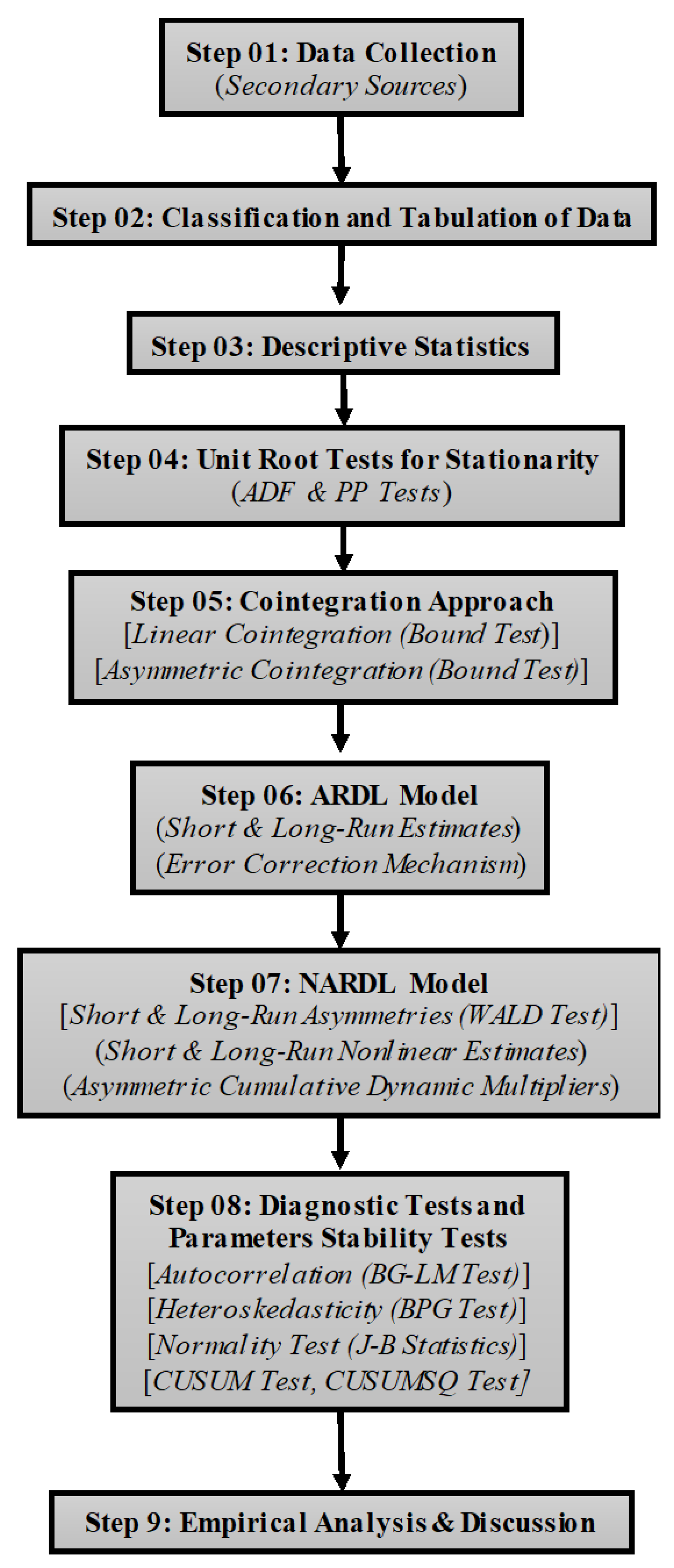
3.2. Methodology
- (i)
- If F-statistic > I(1), we can reject the null hypothesis and conclude the presence of cointegration among the variables.
- (ii)
- If F-statistic < I(0), we failed to reject the null hypothesis and revealed the absence of cointegration among the variables.
- (iii)
- If F-statistic > I(0) and F-statistic < I(1), this implies that the outcome is indecisive.
| Model 3 | Model 4 |
4. Empirical Results
4.1. Preliminary Analysis
4.2. Symmetric and Asymmetric ARDL Estimates
4.2.1. The Symmetric Nexus between Twin Deficit and Energy Inflation
4.2.2. The Asymmetric Nexus between Twin Deficit and Energy Inflation
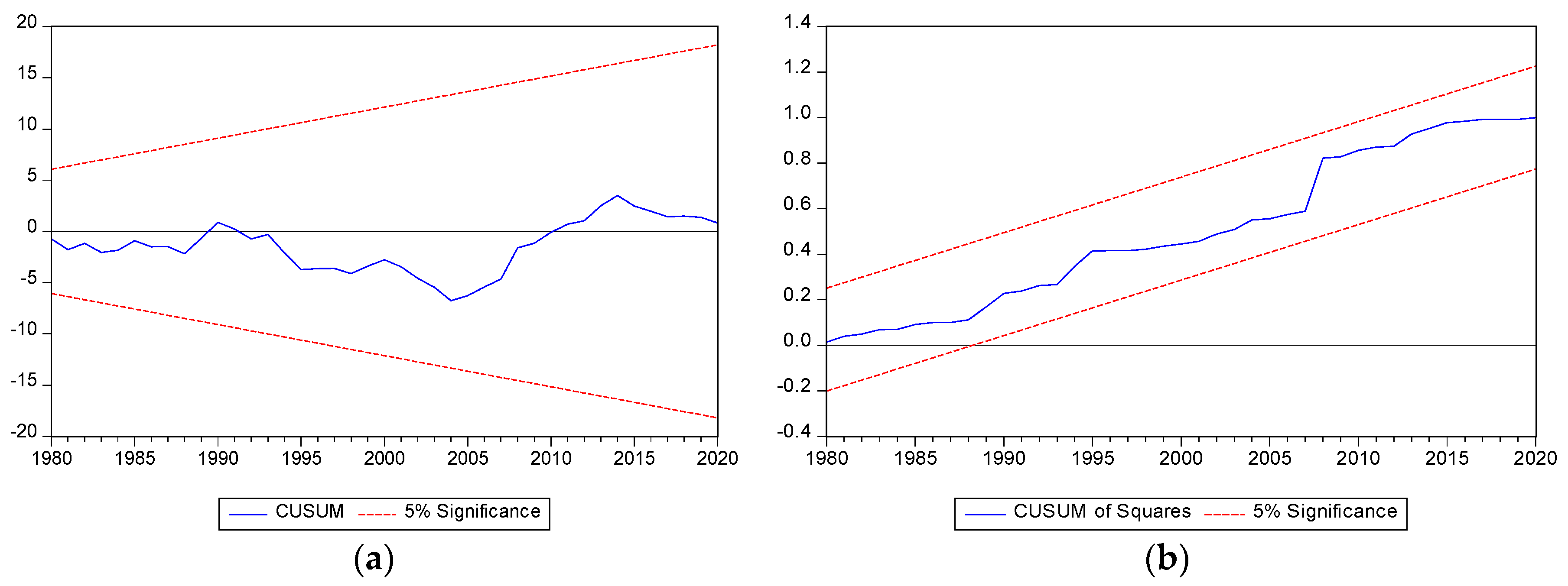
4.3. Diagnostic Checks/Post Estimation Tests and Parameters Stability
Cumulative Dynamic Multipliers
5. Discussion of the Results
6. Conclusions, Policy Implications, Limitations, and Future Research
6.1. Policy Implications
- According to the findings indicated above, the following policy recommendations are proposed by this study.
- First, in order to curtail the favorable effect of the current account deficit and limit its influence on energy prices, authorities should implement policies to limit import payments and stimulate export revenues.
- Second, authorities should broaden the tax base to raise government revenue and stimulate private sector investment in infrastructure projects to mitigate the effect of fiscal deficit on energy prices.
- Third, India’s energy consumption grew dramatically as a result of climate change, exerting upward pressure on prices; thus, to curb energy inflation, the Indian government should execute various initiatives to augment the green environment and reduce energy demand.
- Fourth, in order to curb energy inflation, the usage of renewable energy sources should be fostered.
- Fifth, India has to pursue alternative avenues to purchase oil and gas from the international market at a lower price. Sixth, India needs to stimulate well-planned urbanization as a means of bringing the nation’s energy demand under control.
- Finally, to regulate energy inflation, the RBI also prevents a significant depreciation of the currency, which might exacerbate core inflation.
6.2. Limitations and Future Research
Author Contributions
Funding
Institutional Review Board Statement
Informed Consent Statement
Data Availability Statement
Conflicts of Interest
References
- Ngarava, S. Long term relationship between food, energy and water inflation in South Africa. Water-Energy Nexus 2021, 4, 123–133. [Google Scholar] [CrossRef]
- Norouzi, N. Presenting a conceptual model of water-energy-food nexus in Iran. Curr. Res. Environ. Sustain. 2022, 4, 100119. [Google Scholar] [CrossRef]
- Norouzi, N.; Fani, M.; Talebi, S. Green tax as a path to greener economy: A game theory approach on energy and final goods in Iran. Renew. Sustain. Energy Rev. 2022, 156, 111968. [Google Scholar] [CrossRef]
- Carter, S.; Gulati, M. Understanding the Food Energy Water Nexus Climate Change, the Food Energy Water Nexus and Food Security in South Africa; WWF: Newlands, South Africa, 2014. [Google Scholar]
- Ahmad, T.; Zhang, D. A critical review of comparative global historical energy consumption and future demand: The story told so far. Energy Rep. 2020, 6, 1973–1991. [Google Scholar] [CrossRef]
- Albatayneh, A.; Juaidi, A.; Abdallah, R.; Peña-Fernández, A.; Manzano-Agugliaro, F. Effect of the subsidised electrical energy tariff on the residential energy consumption in Jordan. Energy Rep. 2022, 8, 893–903. [Google Scholar] [CrossRef]
- Carfora, A.; Pansini, R.V.; Scandurra, G. The causal relationship between energy consumption, energy prices and economic growth in Asian developing countries: A replication. Energy Strategy Rev. 2019, 23, 81–85. [Google Scholar] [CrossRef]
- Wang, Z.; Yang, Z.; Zhang, B.; Li, H.; He, W. How does urbanization affect energy consumption for central heating: Historical analysis and future prospects. Energy Build. 2022, 255, 111631. [Google Scholar] [CrossRef]
- Pachar, S. Renewable & Non-Renewable Energy Sources in India: A Study on Future Prospects. Renew. Energy 2020, 29, 8952–8958. [Google Scholar]
- Khan, S.; Haleem, A. Investigation of circular economy practices in the context of emerging economies: A CoCoSo approach. Int. J. Sustain. Eng. 2021, 14, 357–367. [Google Scholar] [CrossRef]
- Ali, S.S.; Kaur, R.; Khan, S. Evaluating sustainability initiatives in warehouse for measuring sustainability performance: An emerging economy perspective. Ann. Oper. Res. 2022, 1–40. [Google Scholar] [CrossRef]
- Amjad, M.A.; Asghar, N.; ur Rehman, H. Investigating the Role of Energy Prices in Enhancing Inflation in Pakistan: Fresh Insight from Asymmetric ARDL Model. Rev. Appl. Manag. Soc. Sci. 2021, 4, 811–822. [Google Scholar] [CrossRef]
- Ogbeide-Osaretin, E.N. Analysing energy consumption and poverty reduction nexus in Nigeria. Int. J. Sustain. Energy 2021, 40, 477–493. [Google Scholar] [CrossRef]
- Abbasi, K.R.; Lv, K.; Radulescu, M.; Shaikh, P.A. Economic complexity, tourism, energy prices, and environmental degradation in the top economic complexity countries: Fresh panel evidence. Environ. Sci. Pollut. Res. 2021, 28, 68717–68731. [Google Scholar] [CrossRef]
- Esen, Ö.; Bayrak, M. Does more energy consumption support economic growth in net energy-importing countries? J. Econ. Financ. Adm. Sci. 2017, 22, 75–98. [Google Scholar] [CrossRef] [Green Version]
- Rubene, I. The role of energy prices in recent inflation outcomes: A cross-country perspective. Econ. Bull. Boxes 2018, 7. Available online: https://ideas.repec.org/a/ecb/ecbbox/201800075.html (accessed on 6 February 2023).
- Murphy, R.G.; Rohde, A. Rational bias in inflation expectations. East. Econ. J. 2018, 44, 153–171. [Google Scholar] [CrossRef]
- Mallick, L.; Behera, S.R.; Murthy, R.R. Does the twin deficit hypothesis exist in India? Empirical evidence from an asymmetric non-linear cointegration approach. J. Econ. Asymmetries 2021, 24, e00219. [Google Scholar] [CrossRef]
- Bilman, M.E.; Karaoğlan, S. Does the twin deficit hypothesis hold in the OECD countries under different real interest rate regimes? J. Policy Model. 2020, 42, 205–215. [Google Scholar] [CrossRef]
- Banday, U.J.; Aneja, R. Twin deficit hypothesis and reverse causality: A case study of China. Palgrave Commun. 2019, 5, 1–10. [Google Scholar]
- Lau, E.; Tang, T.C. Twin deficits in Cambodia: Are there reasons for concern? An empirical study. Monash Univ. Dep. Econ. Disscussion Pap. 2009, 11, 1–9. [Google Scholar]
- Corsetti, G.; Müller, G.J. Twin deficits: Squaring theory, evidence and common sense. Econ. Policy 2006, 21, 598–638. [Google Scholar] [CrossRef]
- Ghatak, A.; Ghatak, S. Budgetary deficits and Ricardian equivalence: The case of India, 1950–1986. J. Public Econ. 1996, 60, 267–282. [Google Scholar] [CrossRef]
- Burney, N.A.; Akhtar, N.; Qadir, G. Government budget deficits and exchange rate determination: Evidence from Pakistan [with Comments]. Pak. Dev. Rev. 1992, 31, 871–882. [Google Scholar] [CrossRef] [Green Version]
- Akanbi, O.A. Fiscal policy and current account in an oil-rich economy: The case of Nigeria. Empir. Econ. 2015, 48, 1563–1585. [Google Scholar] [CrossRef]
- IEA. India Energy Outlook 2021; OECD Publishing: Paris, France, 2021. [Google Scholar] [CrossRef]
- Pundhir, S.K.S.; Agrawal, A.M. Prediction Model for Petroleum Consumption in India using the Best Fit Model concept. In Proceedings of the 2021 5th International Conference on Information Systems and Computer Networks (ISCON), Mathura, India, 22–23 October 2021; pp. 1–6. [Google Scholar]
- Giri, F. The relationship between headline, core, and energy inflation: A wavelet investigation. Econ. Lett. 2022, 210, 110214. [Google Scholar] [CrossRef]
- Andreani, M.; Giri, F. Not a short-run noise! The low-frequency volatility of energy inflation. Financ. Res. Lett. 2023, 51, 103477. [Google Scholar] [CrossRef]
- Kilian, L.; Zhou, X. Oil prices, gasoline prices, and inflation expectations. J. Appl. Econom. 2022, 37, 867–881. [Google Scholar] [CrossRef]
- Hasenzagl, T.; Pellegrino, F.; Reichlin, L.; Ricco, G. A Model of the Fed’s View on Inflation. Rev. Econ. Stat. 2022, 104, 686–704. [Google Scholar] [CrossRef]
- Osoro, K.O.; Gor, S.O.; Mbithi, M.L. The twin deficit and the macroeconomic variables in Kenya. Int. J. Innov. Educ. Res. 2014, 2, 64–85. [Google Scholar] [CrossRef]
- ABBASI, M.A.; AMRAN, A.; REHMAN, N.A.; ALI, A. Twin Deficit and Macroeconomic Indicators in Emerging Economies: A Comparative Study of Iran and Turkey. J. Asian Financ. Econ. Bus. 2021, 8, 617–626. [Google Scholar]
- Handoyo, R.D.; Erlando, A.; Astutik, N.T. Analysis of twin deficits hypothesis in Indonesia and its impact on financial crisis. Heliyon 2020, 6, e03248. [Google Scholar] [CrossRef] [Green Version]
- Premaratne, S.P.; Ravinthirakumaran, N.; Kesavarajah, M. Twin Deficits in Sri Lanka: An Econometric Analysis. Sri Lanka Econ. J. 2011, 12, 31–63. [Google Scholar]
- Lau, E.; Mansor, S.A.; Puah, C.H. Revival of the twin deficits in Asian crisis-affected countries. Econ. Issues 2010, 15 Pt 1, 29–53. [Google Scholar]
- Nautiyal, N.; Belwal, S.; Belwal, R. Assessment, Interaction and the Transmission Process of Twin deficit Hypothesis: Fresh Evidence from India. Bus. Perspect. Res. 2022. [Google Scholar] [CrossRef]
- Anoruo, E.; Ramchander, S. Current account and fiscal deficits: Evidence from India. Indian Econ. J. 1998, 45, 66–80. [Google Scholar] [CrossRef]
- Abbas, S.; Waheed, A. Fiscal deficit and trade deficit nexus in Pakistan: An econometric inquiry. Panoeconomicus 2020, 1–23. [Google Scholar] [CrossRef]
- Dey, S.R.; Tareque, M. Twin deficits hypothesis in Bangladesh: An empirical investigation. Int. J. Emerg. Markets. 2022, 17, 2350–2379. [Google Scholar] [CrossRef]
- Shastri, S. Re-examining the twin deficit hypothesis for major South Asian economies. Indian Growth Dev. Rev. 2019, 12, 265–287. [Google Scholar] [CrossRef]
- Oladipo, S.O.; Akinbobola, T.O. Budget deficit and inflation in Nigeria: A causal relationship. J. Emerg. Trends Econ. Manag. Sci. 2011, 2, 1–8. [Google Scholar]
- Saleh, A.S.; Nair, M.; Agalewatte, T. The twin deficits problem in Sri Lanka: An econometric analysis. South Asia Econ. J. 2005, 6, 221–239. [Google Scholar] [CrossRef]
- Ramakrishnan, R.; Raju, G.R.; Gopakumar, K.U. Analysis of the Sustainability of India’s Current Account Deficit. J. Int. Econ. 2020, 11, 2–18. [Google Scholar]
- Dhar, B.; Rao, K.C. India’s current account deficit: Causes and cures. Econ. Political Wkly. 2014, 41–45. [Google Scholar]
- Manuel, V.; Mbazima-Lando, D.; Naimhwaka, E. Effects of Government Expenditure on Foreign Exchange Reserves: Evidence for Namibia. Int. J. Econ. Financ. Issues 2023, 13, 172. [Google Scholar] [CrossRef]
- Rasool, H. Identifying Inflation Dynamics in India in the Post Reform Period. South Asian J. Macroecon. Public Financ. 2022. [Google Scholar] [CrossRef]
- Okoli, T.T.; Tewari, D.D.; Ileasanmi, K.D. Investigating a threshold effect in Twin Deficit Hypothesis: Evidence from the BRICS Economies. Cogent Econ. Financ. 2021, 9, 1886451. [Google Scholar] [CrossRef]
- Ayinde, T.O.; Ogunsiji, M.O.; Ibikunle, K.O. Twin Deficit Hypothesis and Macroeconomic Fundamentals: New Evidence from Nigeria. Q. J. Econom. Res. 2021, 7, 1–12. [Google Scholar] [CrossRef]
- Knee, K.L.; Masker, A.E. Association between unconventional oil and gas (UOG) development and water quality in small streams overlying the Marcellus Shale. Freshw. Sci. 2019, 38, 113–130. [Google Scholar] [CrossRef]
- Bhat, J.A.; Ganaie, A.A.; Sharma, N.K. Macroeconomic response to oil and food price shocks: A structural var approach to the Indian economy. Int. Econ. J. 2018, 32, 66–90. [Google Scholar] [CrossRef]
- Alom, F.; Ward, B.D.; Hu, B. Macroeconomic effects of world oil and food price shocks in Asia and Pacific economies: Application of SVAR models. OPEC Energy Rev. 2013, 37, 327–372. [Google Scholar] [CrossRef]
- Khan, M.A.; Ahmed, A. Macroeconomic effects of global food and oil price shocks to the Pakistan economy: A structural vector autoregressive (SVAR) analysis. Pak. Dev. Rev. 2011, 50, 491–511. [Google Scholar] [CrossRef] [Green Version]
- Tang, W.; Wu, L.; Zhang, Z. Oil price shocks and their short-and long-term effects on the Chinese economy. Energy Econ. 2010, 32, S3–S14. [Google Scholar] [CrossRef] [Green Version]
- Jones, D.W.; Leiby, P.N.; Paik, I.K. Oil price shocks and the macroeconomy: What has been learned since 1996. Energy J. 2004, 25, 1–32. [Google Scholar] [CrossRef]
- Yuan, J.H.; Kang, J.G.; Zhao, C.H.; Hu, Z.G. Energy consumption and economic growth: Evidence from China at both aggregated and disaggregated levels. Energy Econ. 2008, 30, 3077–3094. [Google Scholar] [CrossRef]
- Shakeel, S.R.; Takala, J.; Shakeel, W. Renewable energy sources in power generation in Pakistan. Renew. Sustain. Energy Rev. 2016, 64, 421–434. [Google Scholar] [CrossRef]
- Yasmeen, H.; Wang, Y.; Zameer, H.; Solangi, Y.A. Does oil price volatility influence real sector growth? Empirical evidence from Pakistan. Energy Rep. 2019, 5, 688–703. [Google Scholar] [CrossRef]
- Iqbal, S.; Yasmin, F.; Safdar, N.; Safdar, M. Investigation of energy inflation dynamics in Pakistan: Revisiting the role of structural determinants. Rev. Appl. Manag. Soc. Sci. 2021, 4, 371–380. [Google Scholar] [CrossRef]
- Talha, M.; Sohail, M.; Tariq, R.; Ahmad, M.T. Impact of oil prices, energy consumption and economic growth on the inflation rate in Malaysia. Cuad. Econ. 2021, 44, 26–32. [Google Scholar]
- Haider, A.; Ahmed, Q.M.; Jawed, Z. Determinants of energy inflation in Pakistan: An empirical analysis. Pak. Dev. Rev. 2014, 53, 491–504. [Google Scholar] [CrossRef] [Green Version]
- Acheampong, A.O.; Boateng, E.; Amponsah, M.; Dzator, J. Revisiting the economic growth–energy consumption nexus: Does globalization matter? Energy Econ. 2021, 102, 105472. [Google Scholar] [CrossRef]
- Wong, B. Do inflation expectations propagate the inflationary impact of real oil price shocks?: Evidence from the michigan survey. J. Money Credit. Bank. 2015, 47, 1673–1689. [Google Scholar] [CrossRef]
- Norouzi, N. Post-COVID-19 and globalization of oil and natural gas trade: Challenges, opportunities, lessons, regulations, and strategies. Int. J. Energy Res. 2021, 45, 14338–14356. [Google Scholar] [CrossRef]
- Kousar, S.; Sabir, S.A.; Ahmed, F.; Bojnec, Š. Climate Change, Exchange Rate, Twin Deficit, and Energy Inflation: Application of VAR Model. Energies 2022, 15, 7663. [Google Scholar] [CrossRef]
- El Anshasy, A.A.; Bradley, M.D. Oil prices and the fiscal policy response in oil-exporting countries. J. Policy Model. 2012, 34, 605–620. [Google Scholar] [CrossRef]
- Eregha, P.B.; Aworinde, O.B.; Vo, X.V. Modeling twin deficit hypothesis with oil price volatility in African oil-producing countries. Resour. Policy 2022, 75, 102512. [Google Scholar] [CrossRef]
- Adedokun, A. The effects of oil shocks on government expenditures and government revenues nexus in Nigeria (with exogeneity restrictions). Future Bus. J. 2018, 4, 219–232. [Google Scholar] [CrossRef]
- Sharma, V.; Mittal, A. Fiscal deficit, capital formation, and economic growth in India: A nonlinear ARDL model. Decision 2019, 46, 353–363. [Google Scholar] [CrossRef]
- Vishal, S.; Ashok, M. Revisiting the dynamics of the fiscal deficit and inflation in India: The nonlinear autoregressive distributed lag approach. Econ. Reg. 2021, 17, 318–328. [Google Scholar]
- Sharma, V.; Adil, M.H.; Fatima, S.; Mittal, A. Asymmetric effect of fiscal deficit on current account deficit: Evidence from India. Vision 2021, 09722629211057221. [Google Scholar] [CrossRef]
- Khan, W.; Sharma, V.; Ansari, S.A. Modeling the dynamics of oil and agricultural commodity price nexus in linear and nonlinear frameworks: A case of emerging economy. Rev. Dev. Econ. 2022, 26, 1733–1784. [Google Scholar] [CrossRef]
- Destek, M.A.; Manga, M. Technological innovation, financialization, and ecological footprint: Evidence from BEM economies. Environ. Sci. Pollut. Res. 2021, 28, 21991–22001. [Google Scholar] [CrossRef]
- Bahmani-Oskooee, M.; Ghodsi, H.; Hadzic, M.; Marfatia, H. Asymmetric relationship between money supply and house prices in states across the US. Appl. Econ. 2022, 1–29. [Google Scholar] [CrossRef]
- Engle, R.F.; Granger, C.W. Co-integration and error correction: Representation, estimation, and testing. Econom. J. Econom. Soc. 1987, 251–276. [Google Scholar] [CrossRef]
- Johansen, S. Statistical analysis of cointegration vectors. J. Econ. Dyn. Control. 1988, 12, 231–254. [Google Scholar] [CrossRef]
- Johansen, S.; Juselius, K. Maximum likelihood estimation and inference on cointegration--with applications to the demand for money. Oxf. Bull. Econ. Stat. 1990, 52, 169–210. [Google Scholar] [CrossRef]
- Pesaran, M.H.; Shin, Y.; Smith, R.J. Bounds testing approaches to the analysis of level relationships. J. Appl. Econom. 2001, 16, 289–326. [Google Scholar] [CrossRef]
- Siddiki, J.U. Demand for money in Bangladesh: A cointegration analysis. Appl. Econ. 2000, 32, 1977–1984. [Google Scholar] [CrossRef]
- Shin, Y.; Yu, B.; Greenwood-Nimmo, M. Modelling asymmetric cointegration and dynamic multipliers in a nonlinear ARDL framework. In Festschrift in Honor of Peter Schmidt: Econometric Methods and Applications; Springer: New York, NY, USA, 2014; pp. 281–314. [Google Scholar]
- Panagiotou, D. Asymmetric price responses of the US pork retail prices to farm and wholesale price shocks: A nonlinear ARDL approach. J. Econ. Asymmetries 2021, 23, e00185. [Google Scholar] [CrossRef]
- Sharma, R.; Kautish, P. Dynamism between selected macroeconomic determinants and electricity consumption in India: An NARDL approach. Int. J. Soc. Econ. 2019, 46, 805–821. [Google Scholar] [CrossRef]
- Van Hoang, T.H.; Lahiani, A.; Heller, D. Is gold a hedge against inflation? New evidence from a non-linear ARDL approach. Econ. Model. 2016, 54, 54–66. [Google Scholar] [CrossRef] [PubMed]
- Pesaran, M.H.; Shin, Y. An autoregressive distributed-lag modelling approach to cointegration analysis. Econom. Soc. Monogr. 1998, 31, 371–413. [Google Scholar]
- Dickey, D.A.; Fuller, W.A. Distribution of the estimators for autoregressive time series with a unit root. J. Am. Stat. Assoc. 1979, 74, 427–431. [Google Scholar]
- Phillips, P.C.; Perron, P. Testing for a unit root in time series regression. Biometrika 1988, 75, 335–346. [Google Scholar] [CrossRef]
- Bahmani, M.; Harvey, H.; Hegerty, S.W. Empirical tests of the Marshall-Lerner condition: A literature review. J. Econ. Stud. 2013, 40, 411–443. [Google Scholar] [CrossRef]
- Kathuria, K.; Kumar, N. Are exports and imports of India’s trading partners cointegrated? Evidence from Fourier bootstrap ARDL procedure. Empir. Econ. 2022, 62, 1177–1191. [Google Scholar] [CrossRef]
- Brini, R.; Amara, M.; Jemmali, H. Renewable energy consumption, International trade, oil price and economic growth inter-linkages: The case of Tunisia. Renew. Sustain. Energy Rev. 2017, 76, 620–627. [Google Scholar] [CrossRef]
- Guo, Y.; Yu, C.; Zhang, H.; Cheng, H. Asymmetric between oil prices and renewable energy consumption in the G7 countries. Energy 2021, 226, 120319. [Google Scholar] [CrossRef]
- Shahbaz, M.; Sarwar, S.; Chen, W.; Malik, M.N. Dynamics of electricity consumption, oil price and economic growth: Global perspective. Energy Policy 2017, 108, 256–270. [Google Scholar] [CrossRef] [Green Version]
- NITI Aayog; RMI. Towards a Clean Energy Economy-Post-COVID-19 Opportunities for India’s Energy and Mobility Sectors. 2020. Available online: https://niti.gov.in/sites/default/files/2020-06/India_Green_Stimulus_Report_NITI_VF_June_29.pdf (accessed on 6 February 2023).
- IRENA. Renewable Power Generation Costs in 2020; International Renewable Energy Agency: Abu Dhabi, UAE, 2020; ISBN 978-92-9260-348-9. [Google Scholar]
- Kumar, J.C.R.; Majid, M.A. Renewable energy for sustainable development in India: Current status, future prospects, challenges, employment, and investment opportunities. Energy Sustain. Soc. 2020, 10, 1–36. [Google Scholar] [CrossRef]


| Variables | Acronyms | Definition | Source | Sign |
|---|---|---|---|---|
| Dependent Variables | ||||
| Oil Prices | OP | Log of oil prices | Energy Information Administration, USA | |
| Electricity Prices | EP | Log of electricity prices | Office of the Economic Adviser, Ministry of Commerce and Industry, India | |
| Independent Variables | ||||
| Fiscal Deficit | CFD | Central government’s fiscal deficit (as a % of GDP) | RBI | + |
| Current Account Deficit | CAD | Current account deficit (as a % of GDP) | RBI | + |
| Control Variables | ||||
| Energy Consumption | EC | Log of renewable energy consumption | BP Statistical Review of World Energy | - |
| Carbon Emissions | CO2 | Log of carbon dioxide | BP Statistical Review of World Energy | + |
| Urbanization | UB | Urbanization (annual % of total population) | WDI | + |
| OP | EP | CFD | CAD | EC | CO2 | UB | |
|---|---|---|---|---|---|---|---|
| Mean | 5.155 | 5.213 | 5.160 | −1.120 | 12.865 | 6.626 | 2.938 |
| Median | 5.189 | 5.190 | 5.080 | −1.200 | 10.231 | 6.716 | 2.749 |
| Maximum | 6.554 | 6.309 | 9.183 | 2.317 | 34.060 | 7.873 | 3.955 |
| Minimum | 2.645 | 4.623 | 2.530 | −4.824 | 2.730 | 5.258 | 2.295 |
| Std. Dev. | 0.893 | 0.469 | 1.505 | 1.34 | 9.295 | 0.825 | 0.560 |
| Skewness | −0.701 | 0.438 | 0.391 | 0.050 | 0.819 | −0.078 | 0.699 |
| Kurtosis | 3.824 | 2.257 | 2.712 | 4.089 | 2.492 | 1.744 | 2.174 |
| J-B Stats. | 5.621 | 2.807 | 1.475 | 2.540 | 6.134 | 3.402 | 5.499 |
| Probability | 0.062 | 0.246 | 0.478 | 0.281 | 0.046 | 0.182 | 0.064 |
| Variables | ADF | PP | Remarks | ||
|---|---|---|---|---|---|
| I(0) | I(1) | I(0) | I(1) | ||
| OP | −2.81 (0.06) | −6.47 *** (0.00) | −2.81 (0.06) | −6.47 *** (0.00) | I(1) |
| EP | −1.84 (0.35) | −6.76 (0.00) | −1.90 (0.32) | −6.76 *** (0.00) | I(1) |
| CFD | −3.04 ** (0.03) | - | −3.05 ** (0.03) | - | I(0) |
| CAD | −3.34 (0.01) | - | −3.32 (0.01) | - | I(0) |
| EC | 10.37 (1.00) | −0.95 (0.76) | 10.05 (1.00) | −3.77 ** (0.01) | I(1) |
| CO2 | −1.58 (0.48) | −3.16 ** (0.02) | −1.54 (0.50) | −2.97 ** (0.04) | I(1) |
| Ub | −1.52 (1.00) | −4.78 *** (0.00) | −1.45 (0.54) | −4.64 (0.00) | I(1) |
| Models | Test Statistic | Value | Null Hypothesis: No Levels Relationship | |||
|---|---|---|---|---|---|---|
| Sig. | I(0) | I(1) | ||||
| ARDL | Model 1 | F-statistic | 7.57 | 10% | 2.49 | 3.38 |
| k | 5 | 05% | 2.81 | 3.76 | ||
| Model 2 | F-statistic | 5.51 | 2.5% | 3.11 | 4.13 | |
| k | 5 | 01% | 3.5 | 4.63 | ||
| NARDL | Model 3 | F-statistic | 7.07 | 10% | 2.22 | 3.17 |
| k | 7 | 05% | 2.5 | 3.5 | ||
| Model 4 | F-statistic | 4.94 | 2.5% | 2.76 | 3.81 | |
| k | 7 | 01% | 3.07 | 4.23 | ||
| Variables | ARDL | NARDL | ||||||
|---|---|---|---|---|---|---|---|---|
| Model 1 (1, 0, 0, 0, 0, 0) | Model 2 (1, 0, 0, 0, 0, 0) | Model 3 (1, 0, 0, 1, 0, 0, 0, 0) | Model 4 (1, 2, 0, 0, 0, 1, 2, 1) | |||||
| Coef. | p-Value | Coef. | p-Value | Coef. | p-Value | Coef. | p-Value | |
| Panel A: Short-run estimates | ||||||||
| ΔCFD | 0.08 * | 0.00 | 0.07 *** | 0.06 | − | − | − | − |
| ΔCFD+ | − | − | − | − | −0.06 | 0.11 | 0.11 ** | 0.04 |
| ΔCFD+−1 | − | − | 0.02 | 0.39 | ||||
| ΔCFD− | − | − | − | − | −0.08 | 0.10 | 0.09 ** | 0.05 |
| ΔCAD | 0.15 * | 0.00 | 0.19 * | 0.00 | − | − | − | − |
| ΔCAD+ | − | − | − | − | 0.10 ** | 0.01 | 0.08 *** | 0.08 |
| ΔCAD+−1 | − | − | − | − | −0.15 * | 0.00 | − | − |
| ΔCAD− | − | − | − | − | −0.23 * | 0.00 | −0.06 | 0.18 |
| ΔEC | −0.04 ** | 0.02 | −0.06 ** | 0.01 | −0.05 * | 0.00 | −0.07 * | 0.00 |
| ΔEC−1 | − | − | − | − | − | − | 0.14 | 0.27 |
| ΔCO2 | 1.99 ** | 0.05 | 3.42 ** | 0.01 | 2.20 * | 0.03 | 1.43 | 0.12 |
| ΔCO2,−1 | − | − | − | − | − | − | 5.81 * | 0.00 |
| ΔUb | 0.61 *** | 0.07 | 0.55 | 0.24 | 0.69 ** | 0.03 | 0.39 | 0.09 |
| ΔUb−1 | − | − | − | − | − | − | 0.83 ** | 0.05 |
| Trend | 0.17 * | 0.00 | 0.27 * | 0.00 | 0.15 * | 0.01 | −0.13 * | 0.00 |
| ECT (−1) | −0.34 * | 0.00 | −0.54 * | 0.00 | −0.46 * | 0.00 | −0.42 ** | 0.01 |
| Panel B: Long-run estimates | ||||||||
| CFD | 0.23 ** | 0.01 | 0.14 ** | 0.04 | − | − | − | − |
| CFD+ | − | − | − | − | 0.14 ** | 0.04 | 0.25 ** | 0.02 |
| CFD− | − | − | − | − | −0.19 | 0.10 | −0.22 | 0.16 |
| CAD | 0.43 * | 0.00 | 0.35 * | 0.00 | − | − | − | − |
| CAD+ | − | − | − | − | 0.33 * | 0.00 | 0.19 *** | 0.06 |
| CAD− | − | − | − | − | 0.49 * | 0.00 | 0.16 *** | 0.09 |
| EC | −0.13 ** | 0.02 | −0.11 * | 0.00 | −0.12 * | 0.00 | −0.17 * | 0.00 |
| CO2 | 5.70 * | 0.00 | 6.28 * | 0.00 | 4.69 * | 0.00 | 8.55 * | 0.00 |
| Ub | 1.78 * | 0.00 | 1.02 * | 0.00 | 1.48 ** | 0.05 | 0.19 *** | 0.09 |
| Trend | 0.48 * | 0.00 | 0.49 * | 0.00 | 0.33 * | 0.00 | −0.30 ** | 0.01 |
| Panel C: Diagnostic tests | ||||||||
| Adj R2 | 0.78 | 0.81 | 0.81 | 0.88 | ||||
| χ2SC | 2.18 | 0.11 | 0.33 | 0.80 | −1.87 | 0.13 | −0.25 ** | 0.02 |
| χ2HET | 1.77 | 0.11 | 1.66 | 0.14 | 0.79 | 0.63 | 0.22 | 0.06 |
| χ2NOR | 0.60 | 0.73 | 0.35 | 0.65 | 0.93 | 0.62 | − | − |
| CUSUM | Stable | Stable | Stable | Stable | ||||
| CUSUMQ | Stable | Stable | Stable | Stable | ||||
| WLR CFD | − | − | − | − | 8.12 * | 0.00 | 20.17 * | 0.00 |
| WSR CFD | − | − | − | − | 0.69 | 0.45 | 1.55 | 0.76 |
| WLR CAD | − | − | − | − | 6.48 ** | 0.04 | 5.19 *** | 0.08 |
| WSR CAD | − | − | − | − | 0.31 | 0.23 | −1.79 *** | 0.09 |
Disclaimer/Publisher’s Note: The statements, opinions and data contained in all publications are solely those of the individual author(s) and contributor(s) and not of MDPI and/or the editor(s). MDPI and/or the editor(s) disclaim responsibility for any injury to people or property resulting from any ideas, methods, instructions or products referred to in the content. |
© 2023 by the authors. Licensee MDPI, Basel, Switzerland. This article is an open access article distributed under the terms and conditions of the Creative Commons Attribution (CC BY) license (https://creativecommons.org/licenses/by/4.0/).
Share and Cite
Asif, M.; Sharma, V.; Chandniwala, V.J.; Khan, P.A.; Muneeb, S.M. Modelling the Dynamic Linkage Amidst Energy Prices and Twin Deficit in India: Empirical Investigation within Linear and Nonlinear Framework. Energies 2023, 16, 2712. https://doi.org/10.3390/en16062712
Asif M, Sharma V, Chandniwala VJ, Khan PA, Muneeb SM. Modelling the Dynamic Linkage Amidst Energy Prices and Twin Deficit in India: Empirical Investigation within Linear and Nonlinear Framework. Energies. 2023; 16(6):2712. https://doi.org/10.3390/en16062712
Chicago/Turabian StyleAsif, Mohammad, Vishal Sharma, Vinay Joshi Chandniwala, Parvez Alam Khan, and Syed Mohd Muneeb. 2023. "Modelling the Dynamic Linkage Amidst Energy Prices and Twin Deficit in India: Empirical Investigation within Linear and Nonlinear Framework" Energies 16, no. 6: 2712. https://doi.org/10.3390/en16062712