Abstract
With the centralization of wind power development, power-prediction technology based on wind power clusters has become an important means to reduce the volatility of wind power, so a large-scale power-prediction method of wind power clusters is proposed considering the prediction stability. Firstly, the fluctuating features of wind farms are constructed by acquiring statistical features to further build a divided model of wind power clusters using fuzzy clustering algorithm. Then the spatiotemporal features of the data of wind power are obtained using a spatiotemporal attention network to train the prediction model of wind power clusters in a large scale. Finally, the stability of predictive performance of wind power is analyzed using the comprehensive index evaluation system. The results show that the RMSE of wind power prediction is lower than 0.079 at large-scale wind farms based on the prediction method of wind power proposed in this paper using experience based on the data of 159 wind farms in the Nei Monggol Autonomous Region in China and the extreme error is better than 25% for the total capacity of wind farms, which indicates high stability and accuracy.
1. Introduction
The sharp decline in storage of fossil energy sources has resulted in a new energy revolution all around the world. It has become a new consensus that renewable energies need to be embraced speedily. Wind power is used in large-scale as a new source that is pollution-free and low-carbon in the field of electricity generation with renewable energies. The global capacity of wind fans has reached 837 GW by the end of 2021 and wind power is transforming from a standby power to a main power source [1]. Wind power is an intermittent power source and its volatility and intermittency adversely affect the safe and stable operation of power systems. The accurate prediction of wind power is the basis for power systems to formulate a reasonable dispatch plan, which is conducive to improving the safety and economic operation of the power systems and promotes the consumption of wind power [2].
From the spatial scale, the current research on the level of wind farms is extensive. The output power of a single wind farm can be used as a prediction target. Simple power prediction for a wind farm on its own is not sufficient for a power system to dispatch from the perspective and demand of grid dispatch. On one hand, dispatchers pay more attention to the amount of uncertain power in the entire power system when arranging the operation mode and rotating backup rather than to single wind farms. On the other hand, the increase in penetration power of wind power increases the difficulty in controlling the dispatch in real-time and exchange power of tie lines. So, the power prediction of the wind power clusters is more conducive to formulate a dispatch plan [3].
The methods for power prediction of wind farm clusters [4] mainly include superposition [5], matching methods of spatial resources, and statistical scaling methods [6]. The superposition can directly integrate the results of power prediction of all wind farm clusters involved as soon as it is applied to small wind farms that are sparsely distributed because of simplicity and economy with low prediction accuracy [7]. The matching method of spatial resources, based on a large amount of historical data obtained by extrapolation from similar historical data [8], firstly divides the wind farm clusters into several sub-regions according to the correlation of wind farm resources and grid topology [9]; then it analyzes the similarity between the predicted data of numerical weather [10] and the data of historical meteorological phenomena [11] for every region. The dataset of historical wind speed with the highest similarity with the predicted wind speed was selected as the analysis object and a moving average model was established [12]. Wind power is predicted based on kernel functions [13], regression, and related methods [14] using historical data. The total prediction power is obtained by adding the value predicted within the scope of power prediction of every region. The advantage of the matching method of spatial resource is that it does not need to select a standard wind farm [6] because it only considers the correlation of wind speed. The correlation of wind direction and temperature of wind farms is neglected. In addition, it is highly dependent on historical data, so the predicted result may contain errors [15]. In order to further improve the prediction accuracy of these methods, a statistical scaling method based on statistical techniques and spatiotemporal correlation is proposed [16], which can be used for regional wind power forecasting. In this approach, the entire wind farm cluster is divided into several sub-regions. Wind farms with strong correlation and high prediction accuracy of power are selected as representatives of every region, and the weighting coefficient of each zone is calculated using statistical methods. Then the power of total region is predicted using superposition [17]. However, the method lacks the analysis and utilization of factors related to inter-zonal wind power and with the weighting coefficient it is difficult to objectively reflect the change in operating conditions, so the prediction accuracy is lower.
In addition, Liu et al. [18] propose a regional forecasting method of wind power based on adaptive subareas and long-term and short-term matching. The power of the total region is evaluated during every time frame by adding the predicted power of every subregion. The prediction accuracy of this method depends on the quality of historical data because the correlation among wind farms of wind farm clusters is not considered. Lobo et al. [19] propose a matching method of single-feature relationship to construct the result of total power. Qu et al. [20] propose extracting the correlations of different features from the data of several wind power clusters and express and standardize vine genealogy, combining it with segmented cloud to build the target model. The algorithm is robust enough to compensate for the complex implementation process. Damousis et al. [21] propose a genetic fuzzy model that uses a set of weather stations surrounding a cluster of wind farms with a radius exceeding 15 km to predict the change in wind speed in different time windows in the future. Jursa et al. [22] propose a technique that can select the input parameters and internal model parameters automatically based on particle swarm optimization and the technology that is assessed with the data of 30 wind farms in the extended area. Kumari et al. [23] propose a deep mixed approach to predict solar irradiance. Meanwhile, a spatial characteristic matrix is generated using a single correlation analysis method with long short-term memory (LSTM) neural networks to extract features and convolutional neural networks (CNNs) to predict solar irradiance.
In previous studies, the overall research direction of cluster prediction has been fully studied, especially the improvement of prediction models and algorithms, while the current research questions that are waiting to be solved are as follows:
- The current prediction methods for wind power clusters are mostly optimized for small and medium-sized enterprises, while the prediction methods for large-scale wind power clusters have not been fully developed yet. In fact, the power prediction results of large-scale wind farms are of greater significance for the dispatch in regional grids.
- Different from the power prediction mode of a single wind farm, the input data of the wind power cluster prediction is a data set that is provided by a single wind farm. Additionally, the data divergence is difficult to express in the power feature of wind power clusters directly. It is necessary to further extract the mode of characterizing the output of the wind power cluster from the data set of single wind farm.
- The modeling efficiency of a large number of large-scale wind farms decreases as the number of wind farms increases. Therefore, an urgent problem to be solved is how to improve the efficiency of these models.
Based on the above analysis, this paper proposes an ultra-short-term prediction method for wind power of massive wind power clusters based on feature mining of spatiotemporal correlations. The main contributions of this method are as follows:
- Through the construction of statistical features to describe the fluctuation feature of wind farms, the 159 wind farms are divided into several wind power clusters in the region using a fuzzy clustering algorithm to simplify the number of models aiming at every wind power cluster.
- The data of wind power clusters is reduced in dimensionality using the Kernel principal component analysis algorithm and combined with an average sequence that can reflect the meteorological attributes of wind power clusters in a region to form a spatiotemporal feature representation matrix to reduce the dimensionality of data and accelerate the model convergence in the training stage.
- Under the Seq2Seq framework, a spatiotemporal attention neural network is constructed and key features are dynamically given important attention in the model training stage to improve the training accuracy.
2. Ultra-Short-Term Forecasting Method for Large-Scale Wind Power Clusters
2.1. Sub-Regional Division of Large-Scale Wind Power Clusters
2.1.1. Necessity Analysis of Cluster Division
The behavior of atmospheric circulation from different regions is consistent with the overall behavior of atmospheric circulation. Meanwhile, the change in weather from different regions expresses special characteristics duo to the influence of local effects and the time lag of atmospheric motions. The change in wind power is completely determined by weather conditions. The wind power in a region maintains regularity under the atmospheric movement, i.e., it is a combination of trends and special characteristics, and different wind farms shows differences compared to each other [24].
The traditional wind power prediction theory holds that the smaller the prediction unit, the more complete the information of the predicted result it holds. A single wind farm obtains accuracy of predicted results by adding predictions under the influence of regional smoothing effects [25]. At the moment, the minimum prediction unit of a prediction system for provincial wind power is a single wind farm and the provincial prediction results from every single wind farm are added. In fact, the smaller the predicted unit becomes, the more violently high-frequency pulsatile it seems. However, the random fluctuations of numerical weather predictions (NWP) are obscured by local effects. So, the fluctuation of a predicted model is difficult to distinguish. Such a random fluctuation will be smoothed over by wind farm clusters that have similar power features. The output curves are smoother in macroscopic regional wind farms with stronger tendencies. If the regional wind farms are divided effectively and built models exclusively aim at particular power features of wind farm clusters, the efficiency of the built model will be improved under the predicted accuracy [26].
2.1.2. Fuzzy Clustering
Fuzzy clustering analysis is widely used. Compared to the traditional hard clustering method, the concept of membership degree is introduced in fuzzy clustering. A sample can be divided into several disjoint subsets according to several memberships that belong to different clusters. The matrix of observation data is shown in Equation (1):
In Equation (1), xj = [xi1, xi2, …, xib], xib is the bth observed result of ith sample. i = 1, 2, …, n. s is the quality of the variable.
The objective function is defined as shown in Equation (2):
where V is the matrix of the cluster’s center, V = [V1, V2, …, Vc], c is the quality of the cluster’s center, U = (ujk)c×M is the matrix of membership, ujk is the kth sample which is named, xk is the subordinate to the membership of the type of the jth sample, djk = ‖xk − vj‖ is the Euclidean distance between sample xk and cluster center vj. M is the quality of the sample.
Fuzzy clustering is based on initialized cluster centers and works by continuously updating the matrix of membership and cluster center. Additionally, the minimum of the objective function is optimized to get a divided category. The updating methods of cluster centers and memberships are shown as Equations (3) and (4); l is the number of iterations.
2.1.3. Cluster Division of Wind Power
Representative input characteristics are the fundamental conditions necessary to ensure the convergence of the algorithm. The fluctuating characteristics of wind farms are characterized using statistical feature construction. The fluctuating characteristics are taken as input and the fuzzy clustering algorithm is used as a classifier to realize the division of wind power clusters. The construction schemes of fluctuation characteristics of wind farms are as follows:
- The first statistical feature is the per unit of the maximum output of a wind farm, which represents the maximum output level of the wind farm;
- The second statistical feature is the maximum of wind speed of a wind farm, which reflects the maximum of wind speed of the wind farm;
- The third statistical feature is the power variance of a wind farm, which reflects the power fluctuation of the wind farm;
- The fourth statistical feature is the variance of wind speed in a wind farm, which reflects the fluctuation of wind speed in the wind farm;
- The fifth statistical feature is the average of wind speed, reflecting the distribution of average wind speed;
- The sixth statistical feature is the average per unit of power, which reflects the average distribution of power;
Taking these 6 statistical characteristics of 159 wind farms as input, the fuzzy clustering algorithm was used to divide them into several wind power clusters.
2.2. Power Forecast of Large-Scale Wind Power Clusters
2.2.1. Spatiotemporal Attention Neural Network Algorithm
Under the Seq2Seq framework, a spatiotemporal attention neural network was constructed. In the encoding–decoding structure, the attention mechanism is introduced from two dimensions of space and time to improve the level of attention for spatial characteristics and temporal characteristics in the stage of training the model. STAN provides the spatiotemporal context vector that is aligned directly with the output of the variables. The spatial attention alone is designed with time parallels of attention in the decoder layer to pay attention to the time steps which is the most relevant step and the variable that is most important. Meanwhile, the inputs of the spatial and temporal attention are spatial embeddings and temporal embeddings separately, and the generation of temporal and spatial embeddings is independent of each other [27].
Multivariable time series are provided with the number of features being N, X = [X1, X2, … XN]T ∈ RN×k, whereby k represents the length of the input sequence. Additionally, xi = [x1i, x2i, …,xki], i ∈ {1, 2, …, N}, whereby xi means the input of time series that is the ith input variable.
For each feature xi = [x1i, x2i, …, xki]T, i ∈ {1, 2, …, N}, the spatial embedding is calculated using a feedforward neural network. As for the input of data X = [X1, X2, …, XN]T, the embedded calculation result of all input variables is D = [D1, D2, …, DN]T. As for the time steps X = [X1, X2, …, Xk], the time step embedding H is calculated by coding layers with LSTM, that is two layers, H = [h1, h2, …, hk].
The weight value of spatial attention is calculated using the feedforward neural network as an alignment model. As for the output of time steps j, the ith spatial attention weight βji is described in Equations (5) and (6):
Hereby, , is the state of a hidden layer for the LSTM decoder. represents the ith attention of spatial embedding. Furthermore, the context vector gj can be calculated by the weight value of the spatial attention weight.
For the output j of the time steps, the weight value of time attention can be calculated by aligning model calculations and time attention weight to correspond to ht; is the function containing ht and the last state of the hidden layer . This is shown in Formula (7):
where . Furthermore, the weight value of attention is calculated using the spatiotemporal context vector sj. Spatial and temporal attention depends on the state of the hidden layer of the LSTM decoder—LSTMG and LSTMS. When the context vector gj is calculated, the state of the hidden layer and the neuron of LSTM is defined as and , respectively. For the output of time steps, j, the gj is calculated using the statement of the decoder of the hidden layer as input in spatial attention. The can be acquired by splicing and . The statement of the hidden layer is updated by inputting to LSTMG. Formula (8) is as shown below:
As for the time context vector sj of LSTM, the hidden layer and the neuron of LSTM are and , respectively. As for the time step j, represents the time attention of the context vector to calculate the time. The statement of the hidden layer is updated by inputting and after splicing them to LSTMS. As shown in Formula (9)
the last step is the hidden state of two LSTM updates and connects to as predicted. The calculation process of Spatial–temporal attention weight for time step j is shown in Figure 1.
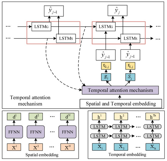
Figure 1.
Spatial–temporal attention weight calculation for time step j.
2.2.2. Wind Power Cluster Power Forecasting
The spatial–temporal fusion data structured is the input coming from the STAN model which is the predictor. The steps are as follows:
- Combining speed, temperature, and humidity of wind farm clusters, the several features whose contribution rates to principal components are higher than those of other features are spatial fusion features such as speed, temperature, and humidity after dimension reduction using principal component analysis.
- The average value of speed and historical power is the second type of statistical characteristic. Supposing the current time is t and the number of features is k, every input of feature will be taken 16 steps forward. That is, the feature at the time point will be used as input.
The data structure of the spatiotemporal characteristics is shown in Figure 2:
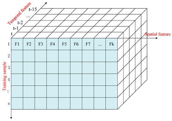
Figure 2.
Space−time feature matrix.
The final wind cluster power prediction framework of wind cluster power is shown in Figure 3 and the following steps are as follows:
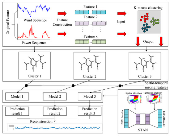
Figure 3.
Wind power cluster forecasting framework.
- The fluctuation characteristics of wind farms are characterized according to the statistical characteristics of meteorological and historical power structures. The input of features is clustered using a K-Means algorithm to divide farms into wind power clusters.
- The wind speed, temperature, and humidity of each wind power cluster are reduced in dimensionality using principal component analysis combining the average values of wind speed, temperature, humidity, and air pressure to construct a spatial feature set.
- The spatiotemporal attention network is built to divide the training set and the test set. The ultra-short-term model of power prediction can be obtained by training the spatiotemporal attention network with the training set.
- The result predicted for a given wind power cluster is added to construct the result predicted for the wind power base;
- Combining this with a comprehensive index of an evaluation system, the accuracy and stability of the ultra-short-term results of power prediction for large-scale wind power clusters are comprehensively evaluated.
2.2.3. Assessment of Power Supply Stability of Large-Scale Wind Power Clusters
The performance of proposed ultra-short-term prediction model of wind power is assessed using root mean square error, average absolute error and qualified rate. The root mean square error (RMSE) is calculated as shown in Equation (10):
In Equation (10), yi is ith time actual power. is ith time actual power. n is the length of the test set. Cap is the actual operating capacity of actual wind power. Because the actual operating capacity is difficult to be obtained, in this paper, the actual operating capacity is replaced by an installed capacity.
The mean absolute error (MAE) is calculated as shown in Equation (11):
The calculation formulas for qualified rate are shown below:
In Equation (12), Bi are the criteria for the qualification rate. Bi = 0 means the value predicted of the ith sample is eligible. Bi = 1 means the value predicted of the ith sample is not eligible. In addition, the maximum positive error and minimum negative error are used to evaluate extreme error events, and the error is calculated as follows:
The maximum positive error is shown in the equation below:
The minimum negative error is shown in the equation below:
3. Experimental Analysis
An experimental analysis was carried out for large-scale wind power clusters of 159 wind farms in inner Mongolia, including the data of measured power and the data of numerical weather predictions from 1 March 2019 to July 2019, with a data resolution of 15 min. The data do not include curtailment when the wind power is reduced. If the sample of wind power is less than 0, the power will be set to zero.
In order to achieve uniform dimensions and improve the calculation efficiency, the maximum–minimum normalization method is used to normalize the input and output data. By taking a certain feature as an example, the principle of normalization is as follows:
In Equation (16), x′ is the feature vector after normalization. xmin and xmax represent the maximum and minimum of x, respectively.
In the stage of prediction, the predicted results are restored to the original power interval according to the denormalization formula, and the denormalization principle is shown in Equation (17):
The fluctuating characteristics are taken as input and the fuzzy clustering algorithm is used as the classifier to realize the division of wind power clusters. The results of the cluster division are shown in Table 1.

Table 1.
Cluster segmentation results.
Taking cluster No. 1 as an example, the principal component analysis was used to reduce the dimension for the three characteristics wind speed, temperature, and humidity of 32 wind farms in a defined space. The number of principal components was taken as 10. The contribution rate of the principal component of each feature is shown in Figure 4. The first and second contribution rate of principal components of wind speed were relatively high and the sum was higher than 70%, so the first and second principal components of wind speed were taken as inputs of modeling inputs. The first principal component of temperature was higher than 90%, so the first principal component of temperature was taken as the input of modeling. The first principal component of humidity was higher than 70%, so the first principal component of temperature was chosen as the input of m spatial features composed of wind speed, temperature, and humidity modeling. The analysis algorithm of principal component reduces the value of spatial features for wind speed, temperature, and humidity from 96 to 4, which greatly reduces the data dimension, retains the consistency of spatial features, and promotes the convergence of the algorithm.
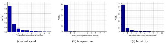
Figure 4.
Principal component contribution rates for different characteristics.
Table 2 shows the training parameters of the data-driven model. To reduce the risk of overfitting, the dropout was set to 0.2.
Table 2.
Training parameters.
The attention weights of the training set of the No. 1 wind power cluster are shown in Figure 5. For the power extrapolation modeling of 16 steps, the spatial attention weights of different prediction steps change little. However, for a certain prediction step, historical power has the highest attention weight, which shows that the autocorrelation of the power series plays a leading role in ultra-short-term power prediction modeling. Then, the first principal component of wind speed and spatial average wind speed also play a leading role in building a model, so the wind speed provided by numerical weather prediction contributes to build model. Strictly speaking, there is a causal correlation between wind speed and wind power; the attention weight of wind speed should be high. However, the causal relationship is diluted in the externalization of attention weight because of the error of numerical weather prediction.
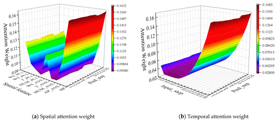
Figure 5.
Spatial–temporal attention weight.
Compared to wind speed and historical power, temperature, humidity, and pressure contribute little to model.
The prediction curves of the 16th step for every wind power cluster and wind power group are shown in Figure 6. The prediction curve of every cluster can accurately track the actual power curve with less error. However, it is worth to be pointed out that the STAN model, like other multi-step prediction models, also has a delay in the time series for its prediction results. The delay becomes more obvious as the prediction step increases. Table 3, Table 4, Table 5, Table 6 and Table 7 explain performance of each wind power cluster.
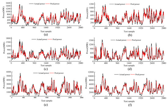
Figure 6.
Predicted power curve: (a) No. 1 cluster prediction curve, (b) No. 2 cluster prediction curve, (c) No. 3 cluster prediction curve, (d) No. 4 cluster prediction curve, (e) No. 5 cluster prediction curve, (f) regional cluster prediction curve.
Table 3.
Cluster performance No. 1.
Table 4.
Cluster performance No. 2.
Table 5.
Cluster performance No. 3.
Table 6.
Cluster performance No. 4.
Table 7.
Cluster performance No. 5.
The prediction indicators of the STAN model are shown in Figure 7. The index of the qualified rate is almost stable at 100%. The absolute error of most sample predictions is less than 25% of the installed capacity. The correlation coefficient and R2 coefficient showed a downward trend with the increase in the predicted time scale. However, they still maintained high values when extrapolated to the 16th step. This indicates that the curve of prediction and actual power maintain the high degree of similarity, and wave peaks and wave troughs can be effectively fitted. The two evaluation indicators of error, MAE and RMSE, have a slight upward trend, which indicates the error is lower in the test set. The RMSE can still be stable within 10% of the installed capacity for the prediction result of the 4th hour. The performance of the power prediction for the STAN model for large-scale wind power clusters is stable.
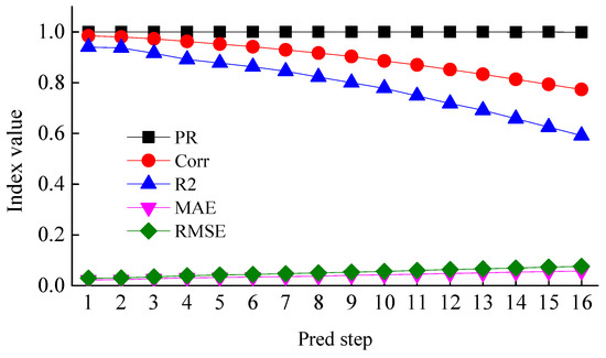
Figure 7.
Overall performance.
Extreme error events have the greatest impact on the power system, and extreme positive errors indicate that the predicted value is seriously lower than the actual value. If the actual output of wind power is higher, the system will be prone to wind abandonment. The extreme negative errors indicate that the predicted value is seriously higher than the actual value. If the actual output of wind power is lower, load shedding events will be prone to occur. The extreme error statistics of the 16-step prediction of the STAN model are shown in Figure 8. According to a description in the literature [28,29], an absolute error that exceeds 40% of the installed capacity is recognized as an extreme error event. According to this statement, comparing the forecast on a single-field basis, extreme error events of wind power clusters are rare in the large scale. As the prediction step increases, the absolute value of the extreme error tends to increase approximately. For the 16th step, the extreme of the positive error of the installed capacity is 25.278%, and the extreme negative error of the installed capacity is 25.719%. They are lower than the described 40% of the installed capacity, so the stability of our STAN model is proven.
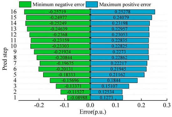
Figure 8.
Extreme error events.
The performance of STAN, a time convolutional network, a long short-term memory network (LSTM), a bidirectional long short-term memory network (BiLSTM), and an LSTM cyclic autoencoder proposed in this paper are compared. As shown in Figure 9, the comparison index is the average RMSE of the predicted result during the 4th in the future. The error is lowest for the STAN algorithm. The TCN algorithm has the lowest performance. The difference between the highest RMSE and the lowest RMSE is 0.00734. However, the total installed capacity of wind power clusters is 16,887 MW. The error between TCN and STAN is 124 MW, which is equivalent to the installed capacity of a small or medium-sized wind farm.
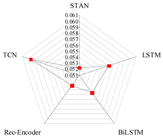
Figure 9.
Comparison of different models.
The performance of the cluster–subcluster prediction result superimposed in this paper, the prediction mode superimposed on the single-field prediction, and the prediction mode directly predicted by the total cluster are compared, and the performance is also the average RMSE of 4 h predictions. The average RMSE of the prediction mode in this paper is 0.0522, the average RMSE of single-field prediction overlay is 0.0618, and the average RMSE of the prediction mode of the direct total cluster is 0.0639. The prediction model proposed in this paper has the lowest error and makes greater contribution to ensuring the power supply capacity of the area.
At the same time, we compare STAN, vanishing gradient mitigation and recurrent neural network (VGM–RNN), sequential floating forward selection feature selection and bidirectional long short-term memory (SFFS–BLSTM), complementary ensemble empirical mode decomposition and multi-scale permutation entropy (CEEMD–MPE), and combining complementary ensemble empirical mode decomposition, multi-scale permutation entropy, least squares support vector machine and particle swarm optimization (CEEMDAN–MPE–LSSVM–PSO). The comparison index is the RMSE of the predicted results in the next 4 h. As shown in Figure 10, compared to other prediction models, the STAN model has the smallest error value and its prediction accuracy is increased by 24.1%, 20.1%, 16.2%, and 10.5%, respectively.
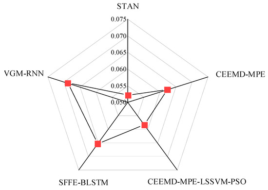
Figure 10.
Comparison of the latest prediction models.
4. Conclusions
- Based on the clustering method of statistical characteristics of wind farms, the output characteristics of wind farms can be effectively identified. Additionally, the wind farm clusters can be divided reasonably.
- The principal component analysis algorithm can realize the extraction of spatial features of wind power clusters, realize the dimensionality reduction of input data, accelerate the training speed of algorithm, and promote the convergence of the algorithm.
- The STAN model can realize rapid modeling and predictions for regional wind power. The RMSE of a test set in the 4th hour is 0.07631 and the extreme error is about 25% of the installed capacity. The qualified rate is close to 100%, and the prediction performance is relatively stable.
5. Research Prospects
Some key information is lost after spatial dimensionality reduction using principal components analysis as well as the physical guidance is lost during cluster division. So, we will further improve the accuracy of data dimensionality reduction. Artificial intelligence and physical knowledge are fused to further improve the rationality of modeling and better serve the development of wind power businesses.
Author Contributions
Methodology, D.H. and D.G.; Formal analysis, T.W.; Investigation, M.Y.; Data curation, C.H.; Writing—original draft, B.W. All authors have read and agreed to the published version of the manuscript.
Funding
This work was supported by the Open Fund of the State Key Laboratory of Operation and Control of Renewable Energy & Storage Systems (China Electric Power Research Institute) (NBY51202201693).
Data Availability Statement
The authors do not have permission to share data.
Conflicts of Interest
The authors declare no conflict of interest.
References
- Yang, M.; Zhang, L.; Cui, Y.; Zhou, Y.; Chen, Y.; Yan, G. Investigating the Wind Power Smoothing Effect Using Set Pair Analysis. IEEE Trans. Sustain. Energy 2019, 11, 1161–1172. [Google Scholar] [CrossRef]
- Peng, X.; Cheng, K.; Lang, J.; Zhang, Z.; Cai, T.; Duan, S. Short-Term Wind Power Prediction for Wind Farm Clusters Based on SFFS Feature Selection and BLSTM Deep Learning. Energies 2021, 14, 1894. [Google Scholar] [CrossRef]
- Mao, Y.A.; Cs, A.; Hl, B. Day-ahead wind power forecasting based on the clustering of equivalent power curves. Energy 2020, 218, 119515. [Google Scholar]
- Huang, S.; Wu, Q.; Guo, Y.; Lin, Z. Bi-level decentralized active and reactive power control for large-scale wind farm cluster. Int. J. Electr. Power Energy Syst. 2019, 111, 201–215. [Google Scholar] [CrossRef]
- Feng, S.; Zhang, G.; Wan, D.; Jiang, S.; Sun, Z.; Zong, Z. On the treatment of hydroelastic slamming by coupling boundary element method and modal superposition method. Appl. Ocean Res. 2021, 112, 102595–102609. [Google Scholar] [CrossRef]
- Valsaraj, P.; Thumba, A.D.; Asokan, K.; Kumar, S.K. Symbolic regression-based improved method for wind speed extrapolation from lower to higher altitudes for wind energy applications. Appl. Energy 2020, 260, 114270–114279. [Google Scholar] [CrossRef]
- Zhang, L.; Gu, T.; Liu, X. Overlapping restricted additive Schwarz method with damping factor for H-matrix linear complementarity problem. Appl. Math. Comput. 2015, 271, 1–10. [Google Scholar] [CrossRef]
- Zhang, Y.; Xiao, F.; Qian, F.; Li, X. VGM-RNN: HRRP Sequence Extrapolation and Recognition Based on a Novel Optimized RNN. IEEE Access 2020, 8, 70071–70081. [Google Scholar] [CrossRef]
- Mu, G.; Guo, G.; Li, J.; Yan, G. The control strategy of energy storage externality for reducing wind curtailment from wind farm cluster. Energy Procedia 2018, 152, 233–239. [Google Scholar] [CrossRef]
- Thang, P.Q.; Kang, W.Y.; Dung, P.Q. A hybrid wind power forecasting model with XGBoost, data preprocessing considering different NWPs. Appl. Sci. 2021, 11, 1100. [Google Scholar]
- Piotrowski, P.; Baczynski, D.; Kopyt, M.; Szafranek, K.; Helt, P.; Gulczynski, T. Analysis of forecasted meteorological data (NWP) for efficient spatial forecasting of wind power generation. Electr. Power Syst. Res. 2019, 175, 105891–105899. [Google Scholar] [CrossRef]
- Pavan, S.K.; Nitin, S.; Richa, N. Short-term wind power prediction using hybrid auto regressive integrated moving average model and dynamic particle swarm optimization. Int. J. Cogn. Inform. Nat. Intell. 2021, 15, 124–151. [Google Scholar]
- Lu, P.; Ye, L.; Tang, Y.; Zhao, Y.; Zhong, W.; Qu, Y.; Zhai, B. Ultra-short-term combined prediction approach based on kernel function switch mechanism. Renew. Energy 2021, 164, 848–866. [Google Scholar] [CrossRef]
- Dong, Y.; Zhang, H.; Wang, C.; Zhou, X. A novel hybrid model based on Bernstein polynomial with mixture of Gaussians for wind power forecasting. Appl. Energy 2021, 286, 116545–116559. [Google Scholar] [CrossRef]
- Ma, Y.; Huang, J. Asymptotic error expansions and splitting extrapolation algorithm for two classes of two-dimensional Cauchy principal-value integrals. Appl. Math. Comput. 2019, 357, 107–118. [Google Scholar] [CrossRef]
- Saint-Drenan, Y.M.; Good, G.H.; Braun, M.; Freisinger, T. Analysis of the uncertainty in the estimates of regional PV power generation evaluated with the upscaling method. Sol. Energy 2016, 135, 536–550. [Google Scholar] [CrossRef]
- Foley, A.M.; Leahy, P.G.; Marvuglia, A.; McKeogh, E.J. Current methods and advances in forecasting of wind power generation. Renew. Energy 2012, 37, 1–8. [Google Scholar] [CrossRef]
- Liu, C.; Zhang, X.; Mei, S.; Liu, F. Local-pattern-aware forecast of regional wind power: Adaptive partition and long-short-term matching. Energy Convers. Manag. 2021, 231, 113799–113812. [Google Scholar] [CrossRef]
- Lobo, M.G.; Sanchez, I. Regional Wind Power Forecasting Based on Smoothing Techniques, with Application to the Spanish Peninsular System. IEEE Trans. Power Syst. 2012, 27, 1990–1997. [Google Scholar] [CrossRef]
- Qu, K.; Si, G.; Yang, Z.; Huang, Y.; Li, P. Correlation modeling of multiple wind farms based on piecewise cloud representation and regular vine copulas. Energy Rep. 2020, 6, 289–297. [Google Scholar] [CrossRef]
- Damousis, I.G.; Alexiadis, M.C. A Fuzzy Model for Wind Speed Prediction and Power Generation in Wind Parks Using Spatial Correlation. IEEE Trans. Energy Convers. 2004, 19, 352–361. [Google Scholar] [CrossRef]
- Jursa, R.; Rohrig, K. Short-term Wind Power Forecasting using Evolutionary Algorithms for Automated Specification of Artificial Intelligence Models. Int. J. Forecast. 2008, 24, 694–709. [Google Scholar] [CrossRef]
- Kumari, P.; Toshniwal, D. Long short term memory–convolutional neural network based deep hybrid approach for solar irradiance forecasting. Appl. Energy 2021, 295, 117061–117081. [Google Scholar] [CrossRef]
- Qin, Y.; Li, K.; Liang, Z.; Lee, B.; Zhang, F.; Gu, Y.; Zhang, L.; Wu, F.; Rodriguez, D. Hybrid forecasting model based on long short term memory network and deep learning neural network for wind signal. Appl. Energy 2019, 236, 262–272. [Google Scholar] [CrossRef]
- Liu, Y.; Tian, R.; Zhang, D.; Zhang, X.; Zhou, J. Analysis and application of wind farm output smoothing effect. Power Syst. Technol. 2013, 37, 987–991. (In Chinese) [Google Scholar]
- Yang, M.; Zhao, M.; Huang, D.W.; Su, X. A composite framework for photovoltaic day-ahead power prediction based on dual clustering of dynamic time warping distance and deep autoencoder. Renew. Energ. 2022, 194, 659–673. [Google Scholar] [CrossRef]
- Gangopadhyay, T.; Tan, S.Y.; Jiang, Z.; Meng, R.; Sarkar, S. Spatiotemporal attention for multivariate time series prediction and interpretation. In Proceedings of the ICASSP 2021–2021 IEEE International Conference on Acoustics, Speech and Signal Processing (ICASSP), Toronto, ON, Canada, 6–11 June 2021; pp. 3560–3564. [Google Scholar]
- Yang, M.; Xu, C.; Wang, K. Ultra-Short-Term Wind Power Forecasting Based on Switching Output Mechanism. High Voltage Eng. 2022, 48, 420–430. [Google Scholar]
- Yang, M.; Xu, C.; Bai, Y.; Ma, M.; Su, X. Investigating black-box model for wind power forecasting using local interpretable model-agnostic explanations algorithm: Why should a model be trusted? CSEE JPES. 2021, 07470. [Google Scholar]


Disclaimer/Publisher’s Note: The statements, opinions and data contained in all publications are solely those of the individual author(s) and contributor(s) and not of MDPI and/or the editor(s). MDPI and/or the editor(s) disclaim responsibility for any injury to people or property resulting from any ideas, methods, instructions or products referred to in the content. |
© 2023 by the authors. Licensee MDPI, Basel, Switzerland. This article is an open access article distributed under the terms and conditions of the Creative Commons Attribution (CC BY) license (https://creativecommons.org/licenses/by/4.0/).