Article

Automated Quantification of Wind Turbine Blade Leading Edge Erosion from Field Images

by
Jeanie A. Aird
1,*,
Rebecca J. Barthelmie
1 and
Sara C. Pryor
2
1
Sibley School of Mechanical and Aerospace Engineering, Cornell University, Ithaca, NY 14853, USA
2
Department of Earth and Atmospheric Sciences, Cornell University, Ithaca, NY 14853, USA
*
Author to whom correspondence should be addressed.
Energies 2023, 16(6), 2820; https://doi.org/10.3390/en16062820
Submission received: 24 February 2023 / Revised: 13 March 2023 / Accepted: 14 March 2023 / Published: 17 March 2023

Abstract

:
Wind turbine blade leading edge erosion is a major source of power production loss and early detection benefits optimization of repair strategies. Two machine learning (ML) models are developed and evaluated for automated quantification of the areal extent, morphology and nature (deep, shallow) of damage from field images. The supervised ML model employs convolutional neural networks (CNN) and learns features (specific types of damage) present in an annotated set of training images. The unsupervised approach aggregates pixel intensity thresholding with calculation of pixel-by-pixel shadow ratio (PTS) to independently identify features within images. The models are developed and tested using a dataset of 140 field images. The images sample across a range of blade orientation, aspect ratio, lighting and resolution. Each model (CNN v PTS) is applied to quantify the percent area of the visible blade that is damaged and classifies the damage into deep or shallow using only the images as input. Both models successfully identify approximately 65% of total damage area in the independent images, and both perform better at quantifying deep damage. The CNN is more successful at identifying shallow damage and exhibits better performance when applied to the images after they are preprocessed to a common blade orientation.

1. Introduction

In 2021, U.S. wind power installed capacity grew by 13.4 GW, representing 32% of the nation’s electric-power capacity additions [1]. Wind turbine rated capacity and dimensions (hub height, rotor diameter) are also increasing. In 2021, the average rated capacity of newly installed wind turbines in the U.S. grew to 3.0 MW, an increase of 9% relative to 2020 [1,2]. Offshore wind turbine dimensions and capacities are also increasing annually, with average capacities of offshore wind turbines totaling over 7 MW and average rotor diameters increasing to 156 m [3]. As wind turbine dimensions and deployment offshore and onshore increase globally and domestically, it is pertinent to quantify longevity and reliability of new and existing wind turbine installations and pursue measures to enhance longevity [4].
Blade integrity is a fundamental determinant of power generation. Blades contribute at least 20% of the overall cost of wind turbines and are also a major source of failures and maintenance costs [5]. Accordingly, an important contributing factor to wind turbine lifespan is leading edge erosion (LEE), which decreases blade performance and longevity, increases maintenance costs, and causes reductions in annual energy production (AEP) [6,7,8,9,10]. Computational modeling may be utilized to estimate the progression of damage along the blade due to hydrometeor impacts and derive estimates for blade lifetime predictions [9,11,12]. Analytical and finite element modeling are being utilized to develop further understanding of materials’ stress from raindrop impacts [7]. Further, computational fluid dynamics (CFD) simulations of leading edge eroded blades show promise for progressing the understanding of the aerodynamic impacts of LEE and forecasting wind turbine operating life [13]. CFD simulations using a 5 MW NREL reference wind turbine model concluded that AEP losses due to leading edge erosion may range between 2 and 3.7%, dependent on the extent and severity of the damage [14]. Severe damage, such as delamination, may result in AEP losses of up to 9% [15]. This reduction in AEP can, in part, be attributed to severe aerodynamic performance reductions attributed to roughness or blade shape changes [16]. Wind tunnel tests with 18% thick commercial wind turbine airfoils (i.e., the vertical thickness of the airfoil is 18% of the distance between the leading and trailing edges of the airfoil) indicate up to a 40% reduction in lift/drag coefficients due to LEE, depending on the erosion pattern and angle of attack [17].
LEE is largely attributable to materials stresses resulting from the impact of hydrometeors (rain, hail) on the rotating blades [18]. The materials stresses are a function of hydrometeor droplet size and impact velocity, angle, and frequency. Analyses using a coupled fluid structure interaction computational model for simulating rain droplet impact on offshore wind turbine blades found that the blade coating had the strongest responses to impacts from larger droplets at impact angles perpendicular to the blade [19]. LEE may then be amplified by icing, lightning, and strong wind gusts that enhance rotor plane turbulence, increase the tip speed and produce irregular aerodynamic loading along the moving blades [3,20,21,22]. Thus, LEE is highly dependent on precipitation and wind climates, wind turbine dimensions and blade materials [23,24]. Higher tip speeds associated with larger wind turbine dimensions may result in increased lifespan losses due to LEE by increasing the closing velocity between the hydrometeors and blade tip [25]. Precipitation-induced LEE risk exhibits high spatial variability across the US, with the highest risks occurring in regions that exhibit more frequent hail (due to increased hydrometeor radii and terminal droplet velocities associated with hail) [26,27].
Estimates of lifetime fatigue predictions for coated substrates are often calculated with the Springer model, which describes the incubation and evolution of erosion as a function of accumulated impacts of rain droplets [28,29,30,31]. During the incubation period, hydrometeor impacts do not result in material loss. Once a threshold level of accumulated impacts is reached, material removal proceeds at an increasing rate with the number of droplet impacts (i.e., pitting damage evolves into cratering damage as droplet impacts increase) [32,33].
In the case of severe damage, blade replacement costs for a single blade can total more than $200,000 [34,35]. Leading edge protection tapes, coatings and/or shells may be employed to reduce damage and LEE-induced aerodynamic losses, but standard leading edge protection tapes may themselves result in AEP losses of nearly 2–3% [36]. Alternatively, ‘erosion safe mode’ operation has been proposed. A study utilizing blade element momentum theory simulations of the Vestas V52 850 kW pitch-regulated variable-speed wind turbine found that reducing the wind turbine’s tip speed during extreme precipitation events resulted in a significant increase in the service life of the leading edge [37].
Early detection of blade damage is necessary to avoid increased maintenance costs as the damage progresses [38,39]. Current techniques for real-time wind turbine blade damage detection include vibration-based techniques [40], ultrasound scanning techniques [41], acoustic emission monitoring [42], and machine vision image or video processing [43]. Three out of four of these methods (acoustic emission, ultrasound, vibration-based techniques) require the use of physical sensors placed along the blade, which are costly and vulnerable to damage in extreme weather conditions [44]. Image processing methods can be used to assess blade conditions from 2D and 3D images or videos captured by instrumentation deployed on unmanned aerial vehicles (UAVs) [45] or taken by technicians. Previous studies investigated supervised machine learning methods to detect blade damage (i.e., an image is assessed for the occurrence of damage [46,47]), but do not investigate the use of automated techniques to quantify the extent and shape of damage along the blade (i.e., calculating the area and expanse of damage). Further, investigation of unsupervised methods to automatically quantify LEE is warranted in the absence of large datasets required for developing supervised machine learning methods.
This work investigates the use of two machine learning methods for automated LEE quantification from a set of 140 field images. The first method is supervised (i.e., learns patterns pre-identified in the data) and employs the use of a region-based convolutional neural network (R-CNN). The second method (PTS) is unsupervised (i.e., identifies repeated patterns using only the statistical properties of the data) and utilizes adaptive pixel intensity thresholding (PT) techniques, k-means segmentation, and calculation of pixel-by-pixel shadow (S) ratios [48,49,50,51]. Both techniques aim to develop models that can be subsequently applied to independent images to automatically quantify the location, areal extent, morphology and type of LEE from field images that have a high dispersion in image characteristics (orientation of the leading edge, extent and types of LEE present within the image, location and aspect ratio of the blade within the image, resolution, lighting conditions, shadow conditions). The objective of this work is to demonstrate the utility of each approach in early and proactive detection and quantification of LEE.

2. Methodology

Four classes of leading edge erosion are generally identified in standards related to damage reporting [52] and are described below ordered by increasing severity in terms of materials loss and AEP degradation (Figure 1):
  • Pitting (shallow): intermittent perforations in the outer blade coating. Pits are generally categorized as shallow, circular cavities. Pits do not expose underlying blade material and generally have minimal impact on aerodynamic performance, particularly compared to more severe damage types such as delamination. However, studies utilizing a S809 airfoil with pitting leading edge erosion indicated that pits have non-negligible impact on aerodynamic performance depending on the pit depth, density and distribution [53]. Pitting erosion may progress into more severe types of erosion (marring, gouges, delamination) with increased numbers of hydrometeor impacts. Pitting may also occur along the chord at short distances from the leading edge.
  • Marring (shallow): surface-level scratches along the outer blade coating, damaging the outermost layers of the coating but not exposing underlying blade material. Marring is generally more severe than pitting, and erosion patterns of marring may be most closely described as Stage 2 erosion in past research and has been shown to cause higher degradation in power production compared to pitting [14].
  • Gouges (deep): deep, circular cavities with removal of the outer blade coating leading to exposure of underlying material. Gouges generally have larger depths and diameters than pits but are not as expansive or deep as delamination [54]. Studies of a DU 96-W-180 airfoil in a wind tunnel showed substantial lift reduction and drag increases for LEE cases with gouges and pits compared to cases with just pits [54]. Gouges may also occur along the chord at short distances from the leading edge.
  • Delamination (deep): the final and most severe stage of leading edge erosion, delamination exposes substantial areas of underlying material. Compared to other leading edge erosion types, delamination generally produces the most severe reductions in aerodynamic performance and may lead to total blade structural failure [14,54,55].
To create a ‘ground truth’ dataset for model development (for the supervised learning approach) and evaluation of both the CNN and PTS models, field images of wind turbine blades are manually inspected for each of these four types of LEE and are annotated accordingly. This process is, to some degree, subjective and may not fully reflect true damage extent, depth and morphology, so the four LEE types are grouped into two broader categories: shallow (pits, marring) and deep (gouges, delamination) (Figure 1).

2.1. Description of Field Images

There were 140 field inspection images of wind turbine blades used to develop and test both damage detection models. The images were taken by technicians using rope access and are extracted from blade inspection reports from a wind farm in the central US over a three-year period. The wind turbines were 8–10 years old when the images were taken. The turbine rated capacity is 1.6 MW, and the rotor diameter is 77 m. The images do not represent a random sample but instead, like the majority of historical inspection imagery, are generally taken when blade damage is suspected or during end of warranty inspection [56]. They differ in terms of the image orientation (i.e., position of the blade within the image), lighting conditions, image resolution, and the presence/absence of other components (i.e., cloud/ground/tower). Most of the images depict a blade section close to the tip, and the amount of visible blade varies in each image. Hence, in the following, the area of damage is given as a percentage of the visible area of the blade, not the total blade area.
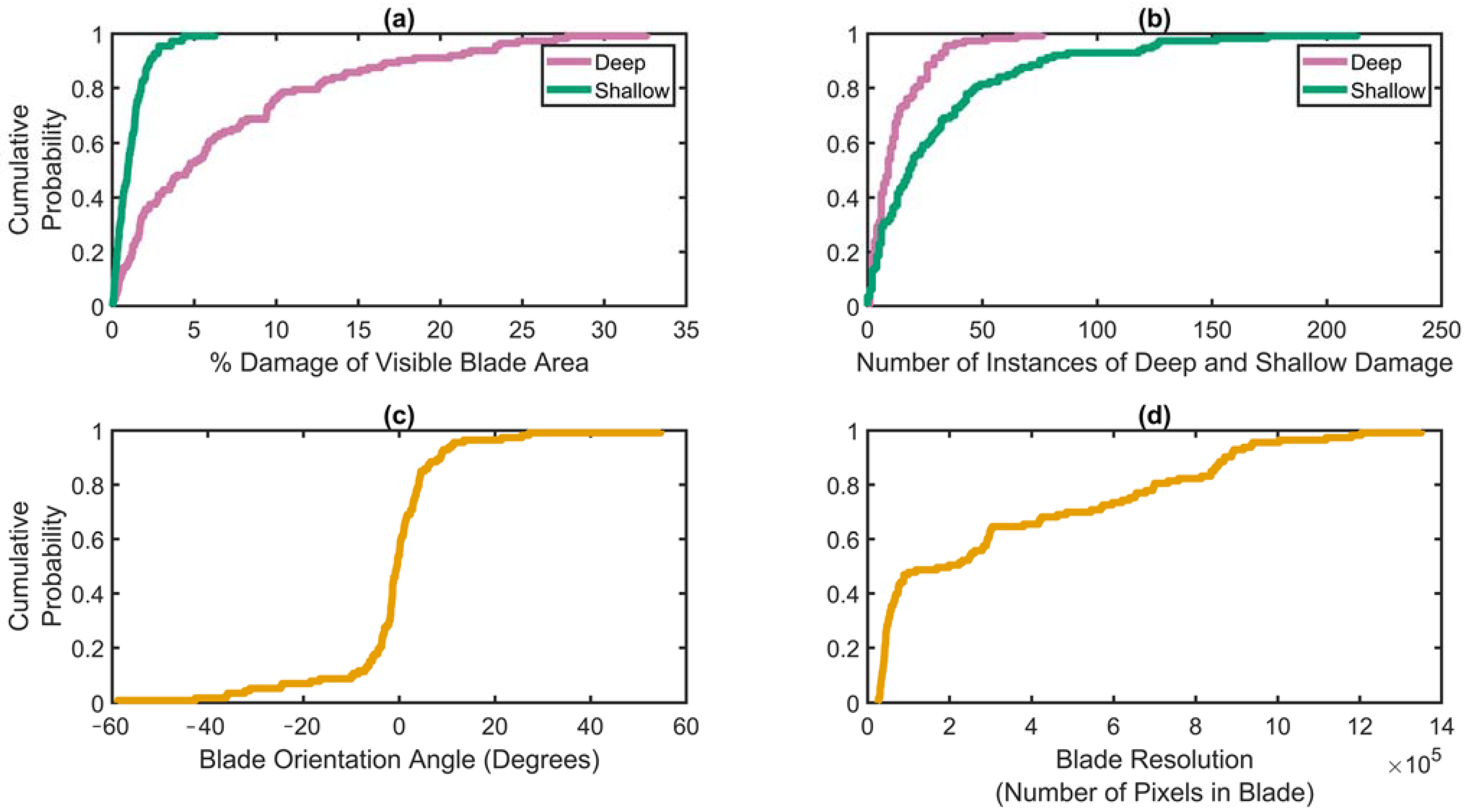
The dataset of images is divided into a 2/3 and 1/3 training and testing split via random sampling, with 1/2 of the testing dataset being utilized to avoid overfitting during training of the supervised machine learning model. Thus, 80 scans are used for training and optimization, while 30 are used for testing and 30 are used to avoid supervised model overfitting. Due to the variations in image quality, blade orientation, and quantity and classification of LEE among the images (Figure 2), single-dimension and two-dimensional (Peacock) Kolmogorov–Smirnov two-sample tests [57] are applied to ensure the training and testing subsets are similar. The results indicate that the randomly sampled subsets (testing, training) are statistically representative of the entire dataset in terms of image resolution, blade orientation, and quantity and classification of LEE.
For the sample of 140 images, there are 2300 and 1200 unique instances of shallow and deep damage. Deep damage generally covers a larger area than shallow damage and tends to occur in fewer but more spatially coherent instances (Figure 2a,b). Over 10% of the blade images exhibit evidence of deep damage over 20% of the visible blade area (Figure 2a). In a few images, up to 30% of the visible blade area exhibits deep damage associated with delamination. Individual images contain up to 200 and 75 unique areas of shallow and deep damage (Figure 2b). In most but not all images, the blade is oriented along the horizontal, with the leading edge being parallel to the x axis of the image (0°) (Figure 2c). Image resolution varied over the three-year period that the dataset was collected (Figure 2d), in part due to use of higher resolution cameras and/or images archiving technology and, to a lesser extent, due to variations in the distance at which the images were taken.

2.2. Workflow

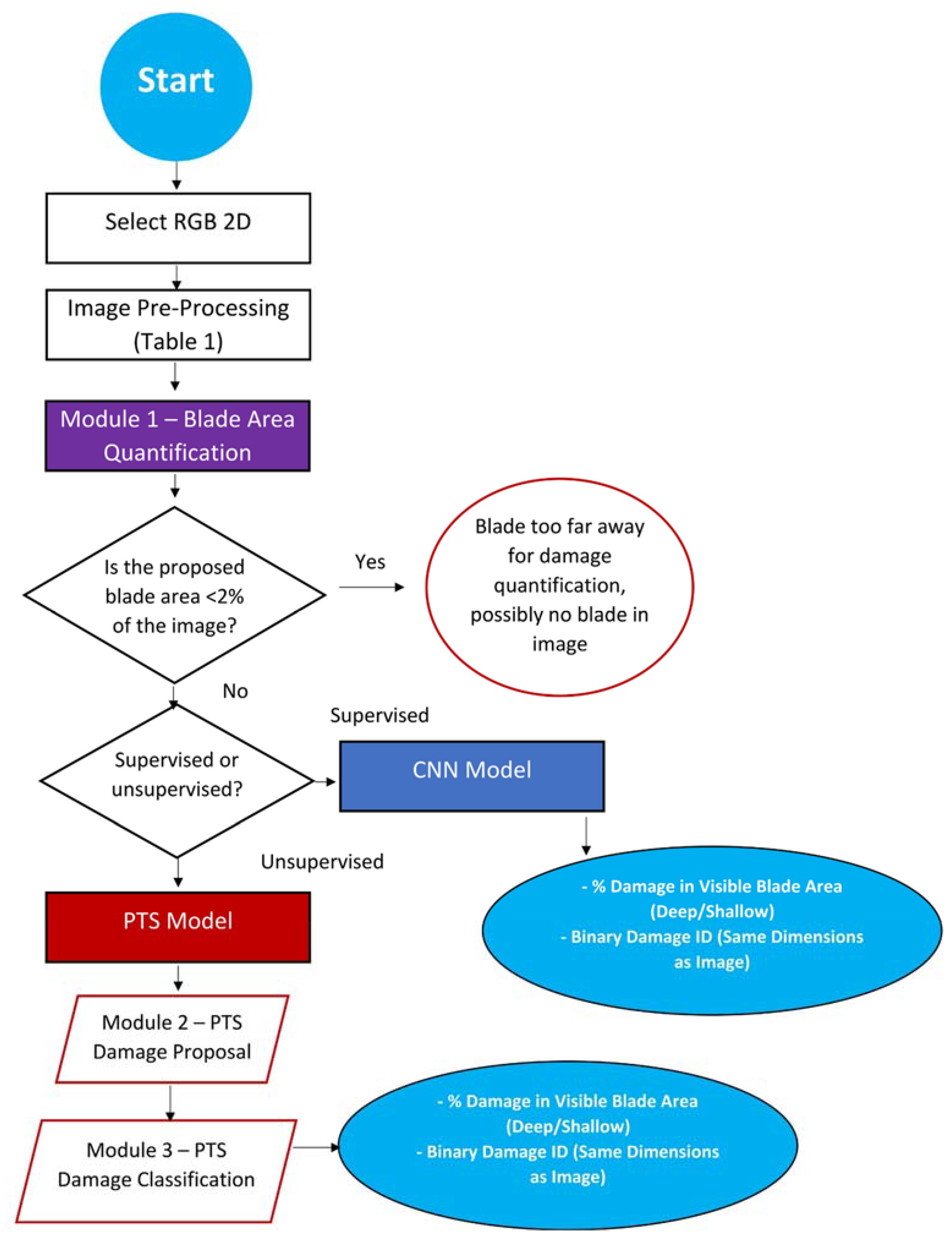
The research described herein adopts to different machine learning frameworks (Figure 3). Supervised machine learning requires use of pre-annotated (ground truth) datasets for model development. In this class of image processing tools, models are trained to identify the features that have been pre-annotated. During training and validation, model weights are adjusted iteratively as more information is supplied from ground truth datasets such that the models can recognize features within images with increased precision. Unsupervised machine learning tools do not require use of pre-annotated images. Instead, data (in this case areas of each image) are segmented into discrete classes where the within class variability is minimized and the between cluster difference is maximized to produce desired outcomes [58]. This work investigates and compares the development of unsupervised (PTS—pixel intensity thresholding and shadow ratio) and supervised (CNN) machine learning models for automated blade leading edge erosion detection, classification and quantification.
The PTS damage classification model and the blade area quantification module employ k-means segmentation (unsupervised clustering applied via the MATLAB imsegkmeans function, R2021a) for damage classification and blade area quantification, respectively. K-means segmentation is used widely for a variety of image processing applications and has demonstrated strength in unsupervised clustering of large and varied datasets [59]. For image processing, k-means segmentation clusters statistically similar pixels and groups these pixels accordingly; thus, the algorithm is ideal for classification use cases [60]. K-means clustering is thus applied herein to (1) locate the blade leading edge by differentiating the blade pixels v. the sky pixels (blade detection module) and (2) identify deep vs. shallow damage (PTS) within the field images.

2.2.1. Image Preprocessing

For both models, a 2D color (RGB, red-green-blue) field image is input; an unsupervised blade detection model is applied to quantify the location of the blade within the image; and binary pixel matrices representing the location and extent of the blade and LEE within the image are output. The first step in the workflow (Table 1, Figure 3) involves taking each 2D RGB image and subjecting it to a series of preprocessing steps: local contrast adjustment, saturation adjustment, and flat field adjustment. The preprocessed images are then used for blade area quantification (BAQ) and other subsequent modules.
The image processing is performed within the MATLAB image processing toolbox, and details of that process are given below.
These pre-processing parameters are optimized (see values given in Table 1) using the training dataset by minimizing the mean square error (MSE) between the modeled blade area within the image or the blade damage with ground truth value for each image:
M S E = 1 N ( E i j O i j ) 2
where N is the total number of pixels in the image, E i j is the binary value of a pixel (in i, j space) in the ground truth (1 = blade or damage, 0 if not), and O i j represents the binary value of the same pixel from the model (1 indicates blade present or damage present).

2.2.2. Blade Area Quantification Module

The input 2D RGB image is first passed through the blade area quantification module (Figure 4) before input into the CNN (supervised) or PTS (unsupervised) modules. For each image:
  • Image details are enhanced through applying a local contrast operation with contrast increased to enhance edge resolution with edge threshold. The edge threshold E specifies the minimum intensity amplitude of strong edges to leave unchanged.
  • Image saturation is enhanced by increasing the saturation value within the HSV (hue, saturation, value) color space through applying a chroma alteration by a factor C. Enhancing the image saturation increases the intensity of blue hues within the image for detection between blade and sky.
  • The pixel-by-pixel illumination invariant shadow ratio φ r is calculated [50,51]. Note this parameter is used both in the blade area quantification module and PTS. The shadow ratio is calculated as follows, utilizing per-pixel (where i, j denotes the pixel location in the image) median-filtered (noise reduction) green (G) and blue (B) color channel values:
    φ r i , j = 4 π arctan B i , j G i . j B i , j + G i . j
    Calculation of the illumination invariant shadow ratio allows for detection of shadows (pixels with highest darkness) throughout a given image, while eliminating ambiguity due to variations in illumination throughout the image. Illumination invariant color spaces are utilized widely in image processing applications and have been shown to reduce image variations due to lighting conditions and shadow, resulting in image color spaces that better describe material properties of objects [61].
  • Shadow ratio values are clustered into two classes (blade or sky) using k-means segmentation.
  • The pixel-by-pixel RGB distance from the RGB pure blue color triplet is calculated using the CIE94 standard and averaged for each proposed class [62]. The class with the lowest/highest average color difference from the blue RGB triplet is designated as the sky/blade, respectively.
At this point, the number of pixels (and their location in the image) in the visible blade area and the background can be determined.
If less than 2% of the pixels in an image are identified in the blade area quantification module as a blade, the image is excluded from further consideration. Otherwise, the image is then passed through either the supervised (CNN) or unsupervised (PTS) model, depending on user preference.

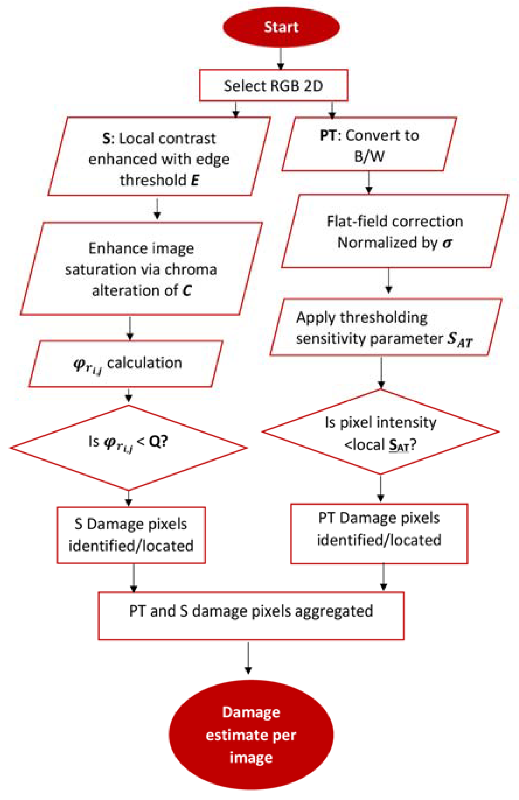
2.2.3. Unsupervised Method: Pixel Intensity Thresholding and Shadow (PTS) Ratio

The PTS model consists of two modules: (1) the damage proposal module and (2) the damage classification module (Figure 4). The damage proposal module has two subcomponents: pixel intensity thresholding (PT) and shadow ratio (S). The PT submodule converts the image to black and white and applies a flat field correction with Gaussian smoothing using a standard deviation of σ to correct shading distortions. Local adaptive pixel intensity thresholding reduces each pixel in the image to a binary value (0 or 1) and segments the foreground and background based on local pixel intensity values [48,63]. The locally adaptive pixel intensity threshold value is specified as a matrix of luminance values and is optimized through use of a sensitivity parameter, S A T (Table 2). Pixels with intensity higher than the adaptive threshold are thus filtered from the image, resulting in a binarized image (1 for damage, 0 for non-damage) for proposed damage pixels.
The S module begins with two preprocessing steps and calculation of the pixel-by-pixel illumination invariant shadow ratio (Equation (2)). The Qth quantile of φ r is then calculated (Q being one of the optimized parameters for the unsupervised models) and pixels with φ r less than the Qth quantile are proposed as damage pixels. The optimization process resulted a threshold for Q of 0.009. Thus, on average, the lowest 0.9% of shadow ratios sampled across all pixels from all the training images are identified as possibly indicating blade damage.
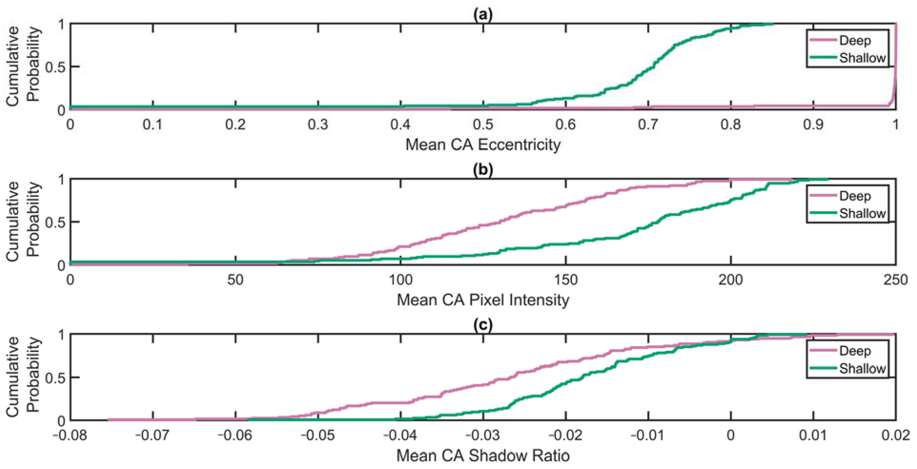
Pixels that are identified in both the PT and S subcomponents as indicating potential damage (i.e., given a proposed damage value of 1) are aggregated and grouped into coherent areas (CA) (connected pixels that share the same binary state). These CA are then input into the damage classification module of the PTS model (Figure 3). Three aspects of the CA are described for shallow and deep damage classes: mean eccentricity (i.e., degree to which the damaged area is elongated along one axis), pixel intensity, and φ r (Figure 5) and clustered into three groups. CAs within each of the three resulting classes are then assigned a label of non-damage, deep, or shallow damage according to the mean shadow ratio of all CAs within each proposed class. Mean shadow ratio across CAs is assumed to be lowest for the deep damage class and highest for the non-damage class. This is based on an assumption that the non-damage class is likely to be blade pixels incorrectly proposed as damage, which should have a higher shadow ratio compared to damage pixels.

2.2.4. Supervised Method—Region-Based Convolutional Neural Network

Convolutional neural networks (CNN) have demonstrated wide success for use in image classification and segmentation tasks, such as facial recognition and object detection in videos and images [64,65,66]. CNNs have been implemented in a wide variety of applications, such as detecting cancerous cells in medical imaging, automated quantification of wind turbine wakes from doppler lidar scans, and object detection from geospatial data such as high-resolution satellite images [67,68,69,70].
This work focuses on the implementation of Mask R-CNN, a state-of-the-art neural network for instance segmentation [71]. We refer to [71] for detailed information about the neural network architecture. Mask R-CNN takes images as input and outputs binary pixel masks for detected objects within the image, thus completing two image processing tasks at once—object classification and segmentation. Generally, task skill for instance segmentation is reported as average precision, which summarizes the shape of the precision-recall curve where:
R e c a l l = T P T P + F N = T P # g r o u n d   t r u t h s
P r e c i s i o n = T P T P + F P = T P # p r e d i c t i o n s
where TP = true positive, FN = false negative, FP = false positive.
Instance segmentations are counted as true positive when the intersection over union (IoU calculates the percentage of predicted pixels that are correctly identified relative to the ground truth pixels) is greater than a prespecified threshold. To convey the model accuracy in such a way that is more relevant in a wind energy context, results are reported in terms of the total percentage of damage pixels correctly identified (i.e., the IoU per image). Generally, the IoU accepted for these tasks is 0.5, (which is the value utilized for the reported average precision values ( A P 50 ) in [71]). The average precision values are much lower when an IoU of 0.75 is utilized as the threshold ( A P 75 ) , indicating that even the state-of-the-art models have difficulty outputting results for instance segmentation with IoU > 0.75. Comparatively, our results are in line with what would be expected from reported results for Mask R-CNN; instance segmentation is challenging, and this is reflected in lower accuracy values than one would expect (particularly for the shallow damage class, which is difficult to detect even subjectively). A study utilizing Mask R-CNN for automated instance segmentation and classification of surgical tools reports similar IoUs to those that are reported in this study [72]. The presented methods could be improved through inclusion of more training data or through iterative improvement of Mask R-CNN. Since the development of Mask R-CNN, studies have shown improvement in average precision values through alteration of the network architecture. Results are improved here by the use of a feature pyramid network (FPN) backbone [73] to enhance CNN performance through improved accuracy in segmentation of objects of varying sizes within the images (particularly important for the shallow damage class which is notably smaller than the deep damage class—Figure 2) and also the use of transfer learning to initialize the CNN weights before training (as in [68,69], weights derived from training the model on the MS COCO dataset are utilized to initialize the neural network).
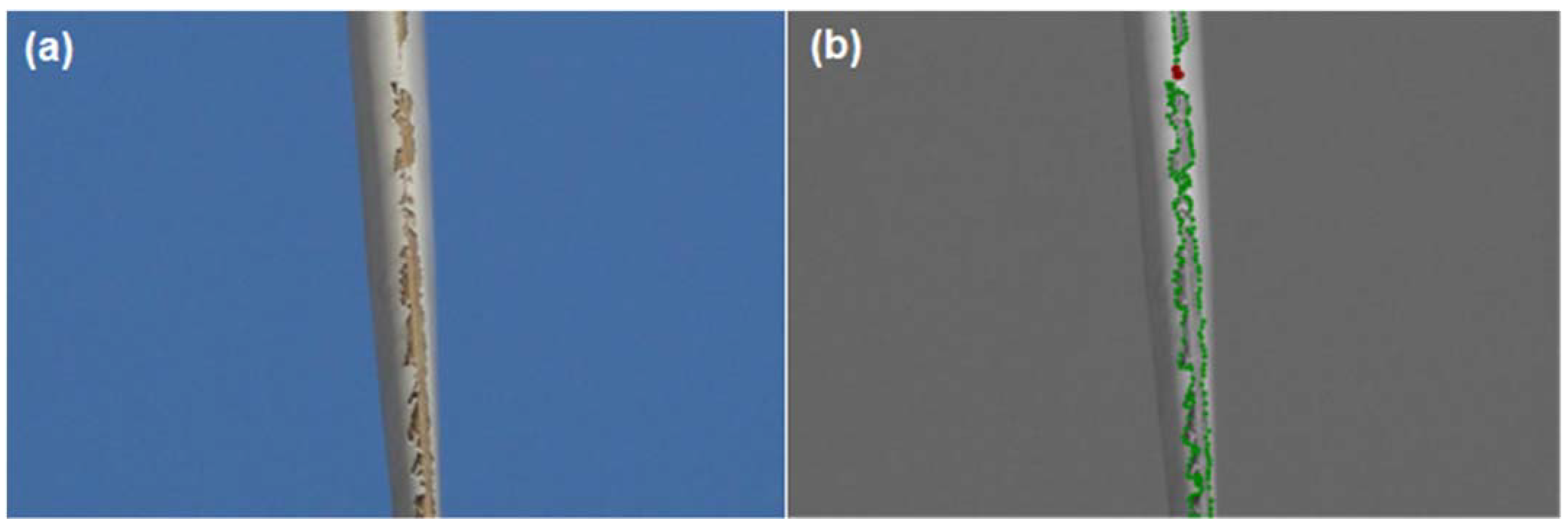
All images are subjectively annotated for the presence of deep or shallow damage along the blade prior to application of the CNN methodology (see example in Figure 6).
Eighty images are used for training the Mask R-CNN model, thirty for validation to prevent overfitting and thirty for testing. Optimal training parameters (learning rate, batch size, epochs—how often the entire dataset is passed through the CNN during training) which minimize classification and segmentation loss are described in Table 3. Sensitivity analyses are also performed to examine whether the model fidelity when applied to the independent test images is strongly determined by (1) use of RBG (C) versus black and white (BW) images or (2) the orientation of the blade within the image. For this second analysis, the images are rotated to ensure consistency of the blade orientation or not (i.e., left as in the raw image) (R denotes rotated or U is unrotated) (Table 4). Previous studies have exhibited sensitivity in CNN results to object orientation, particularly when a robust training dataset of objects in varying orientations is unavailable or limited [68,69]. Further, previous studies conducted during model development in [68,69] indicated that colormap choice and inclusion of color hue (i.e., color images compared to grayscale images) improves CNN results for certain applications. Thus, lowest CNN accuracy/precision rates in LEE quantification and classification may be expected for the CNN trained and tested on black and white, unrotated images ( C N N U B W ) , and highest accuracy/precision rates may be expected for the CNN trained and tested on color images rotated such that the leading edge is horizontal during testing and training ( C N N R C ) . These hypotheses are evaluated in the results section.

3. Results

Results for blade area quantification (Section 3.1), LEE quantification (Section 3.3), and classification (Section 3.4) are given below along with illustrative examples of the original images, subjective damage classification and the results from the supervised (CNN) and unsupervised (PTS) classification methods when applied to the 30 test images (see illustrative examples in Section 3.2). In the following, results are presented as a function of the image resolution in terms of the percent ‘true positives,’ which reflects the fraction of pixels with damage that are correctly identified, while ‘true negatives’ reflect the number of pixels without damage that are correctly identified. The areal extent of damage is expressed as the fraction of blade pixels with damage. When non-damage is quantified, all pixels in the image are used. Higher true negative and true positive values indicate enhanced model fidelity. As described above, the MSE is computed using binary values of damage (1) or non-damage (0) for each pixel in the ground-truth and automated detection methods.

3.1. Blade Area Quantification

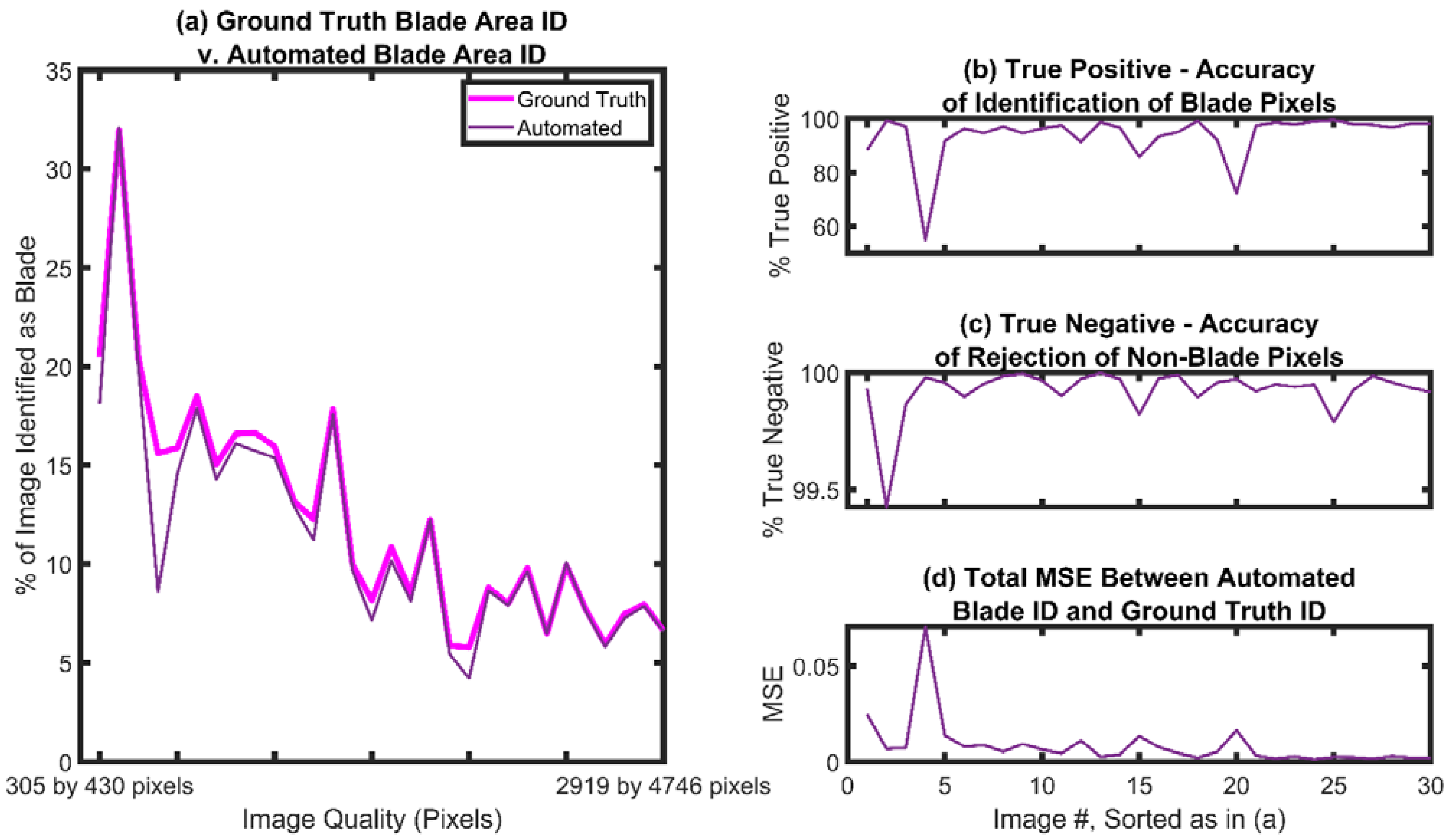
The unsupervised blade area module (Figure 4) accurately identifies a mean of 93.7% of blade pixels per image (averaged over all test images) (Table 5, Figure 7b). The module correctly rejects a mean of 99.9% of non-blade pixels per image, indicating the module has a low propensity for false positives, i.e., identifying non-blade pixels as part of the blade (Figure 7c). The mean subjectively detected blade area over the 30 testing images is 12.34%, while the mean automatically detected blade area is 11.63% (Figure 7a). Total MSE between the automated and subjective blade area detection decreases with increasing image quality (Figure 7d), indicating the benefits of using high-resolution imagery.

3.2. Illustrative Examples of the Representation of Damage Areas: Comparison between CNN and PTS Models

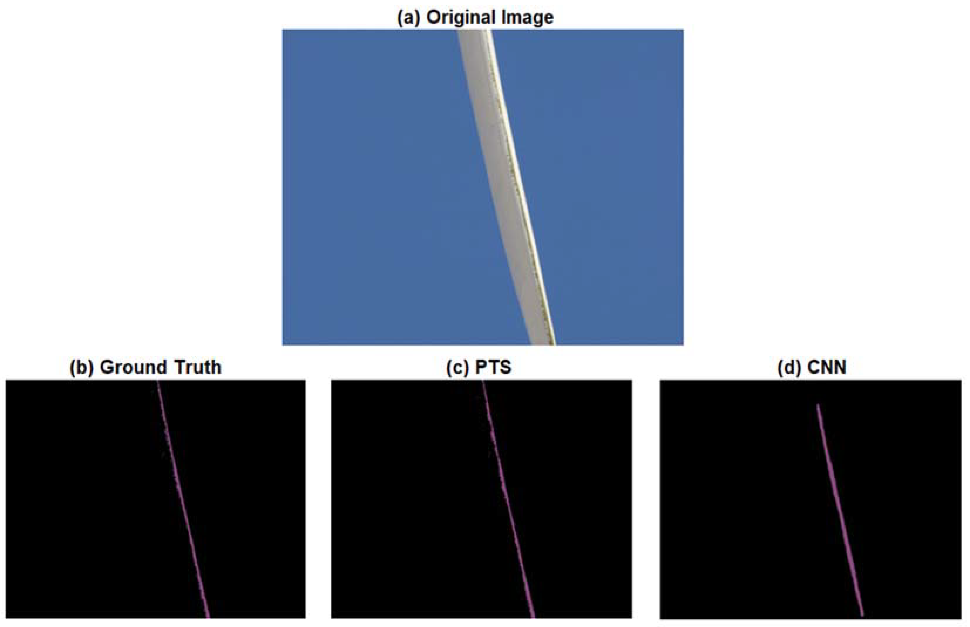
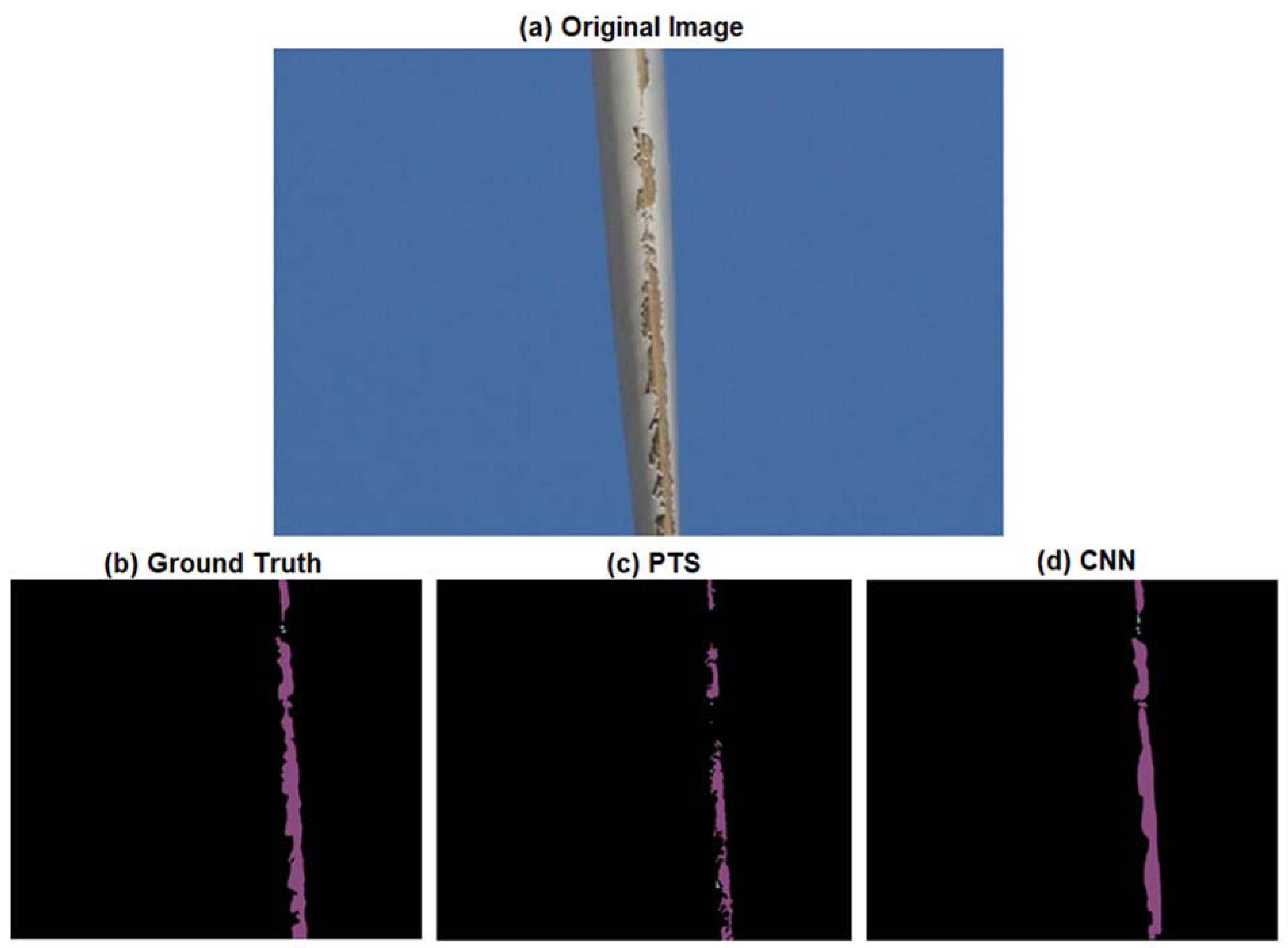
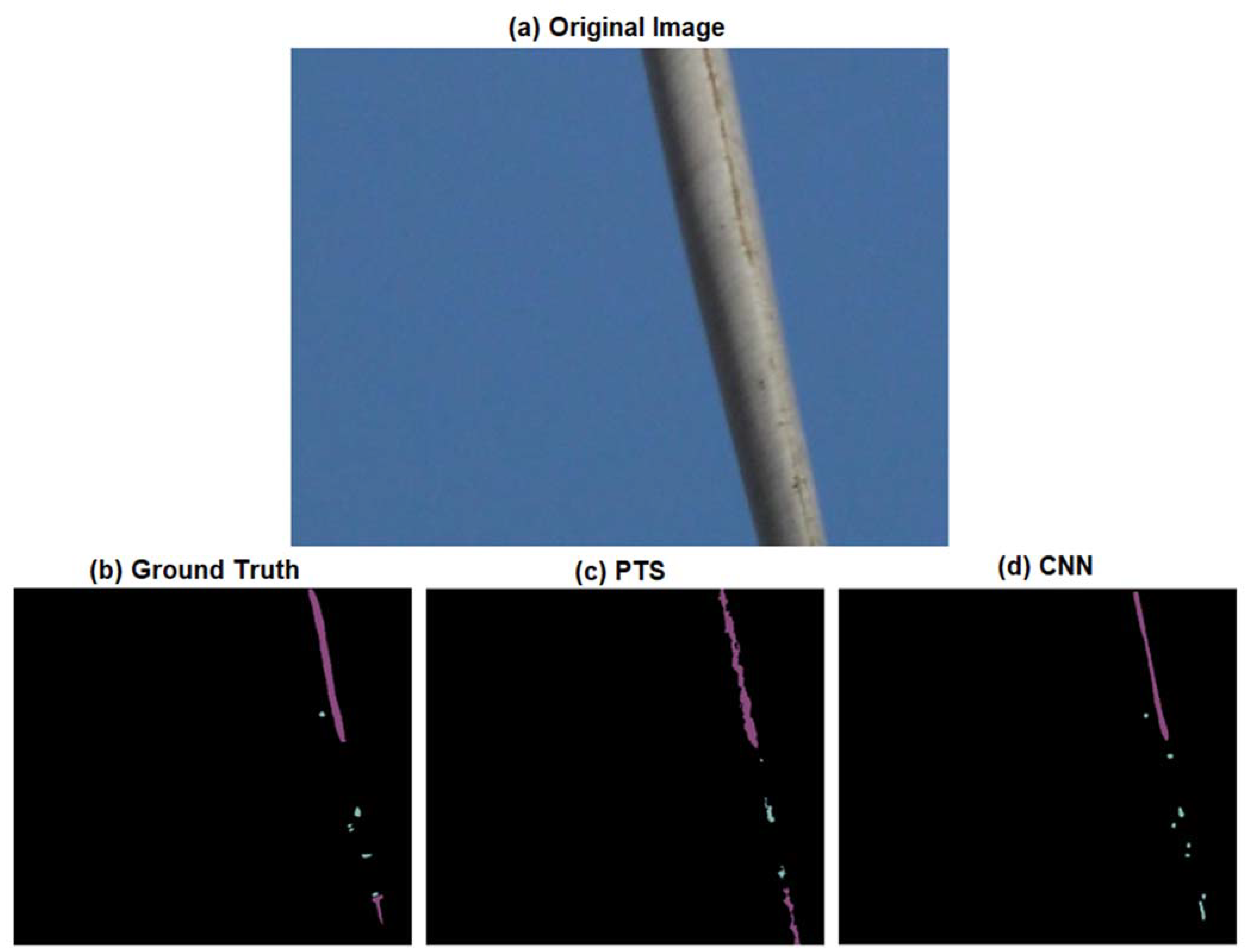
Figure 8, Figure 9 and Figure 10 present illustrative examples of field images in the testing dataset along with the subjective (ground-truth) damage identification, PTS, and CNN LEE quantification and classification results for a range of different damage conditions and image resolution. These indicate similarity in the areas detected as LEE when the damage is fairly coherent along the leading edge (Figure 8). As the damage becomes deeper and less coherent, the CNN appears to better represent the damage as shown in the subjective annotations than the PTS model (Figure 9). Finally, when both deep and shallow damage are present (Figure 10), both models represent the damage area well in addition to detecting different damage types, although the CNN is more adept at representing shallow damage when compared to the PTS model.

3.3. Damage Quantification

Results for the LEE quantification task (proposing pixels of the image as total LEE damage regardless of LEE classification) are presented in this section and summarized in Table 5. The unsupervised PTS module, summarized in Figure 4 and optimized with parameters in Table 1 and Table 2, accurately identifies a mean of 63.9% damage pixels per image (Figure 11b). The PTS module correctly rejects a mean of 99.5% of non-damage pixels per image, indicating the module has a low propensity for false positives, i.e., identifying non-LEE pixels as LEE (Figure 11c). The mean subjectively detected percent area of LEE damage over the 30 test images is 8.9% of the visible blade area, while the mean automatically detected LEE area from the PTS module is 12.0%, indicating a prevalence of false positives associated with the PTS module (Figure 11a). Equivalent results for the CNN indicate 8.7% of the blade is damaged on average. As with the blade area detection, total MSE between the automated PTS and subjective LEE detection decreases with increasing image quality (Figure 11d).
The CNN with the highest accuracy in identifying LEE pixels is C N N R C , while C N N U C exhibits the lowest accuracy. They have a mean accuracy in terms of detecting damage pixels of 65.9 and 58.1%, respectively (Figure 11b). Thus, it appears that rotation of the images on average benefits the detection of damage. Average CNN accuracy (averaged over all four CNNs) in identifying LEE pixels is 61.4%. All four CNNs exhibit low propensity for false positive LEE pixel identification, with average percent true negative across all testing images for all CNNs equaling 99.9% (Figure 11c). As seen with the PTS model, the MSE between automated and subjective LEE identification decreases as image quality increases for all four CNNs. Although the CNN models generate a slightly lower mean areal extent of blade damage than PTS, much closer agreement is found for individual images between any of the CNN models and the subjective damage estimates. The inference is that the CNN model is better able to discriminate between images with low and high damage fractions (Figure 11a). Conversion of the images to black and white prior to application of the CNN does not appear to greatly influence the detection fidelity of CNN.

3.4. Damage Classification

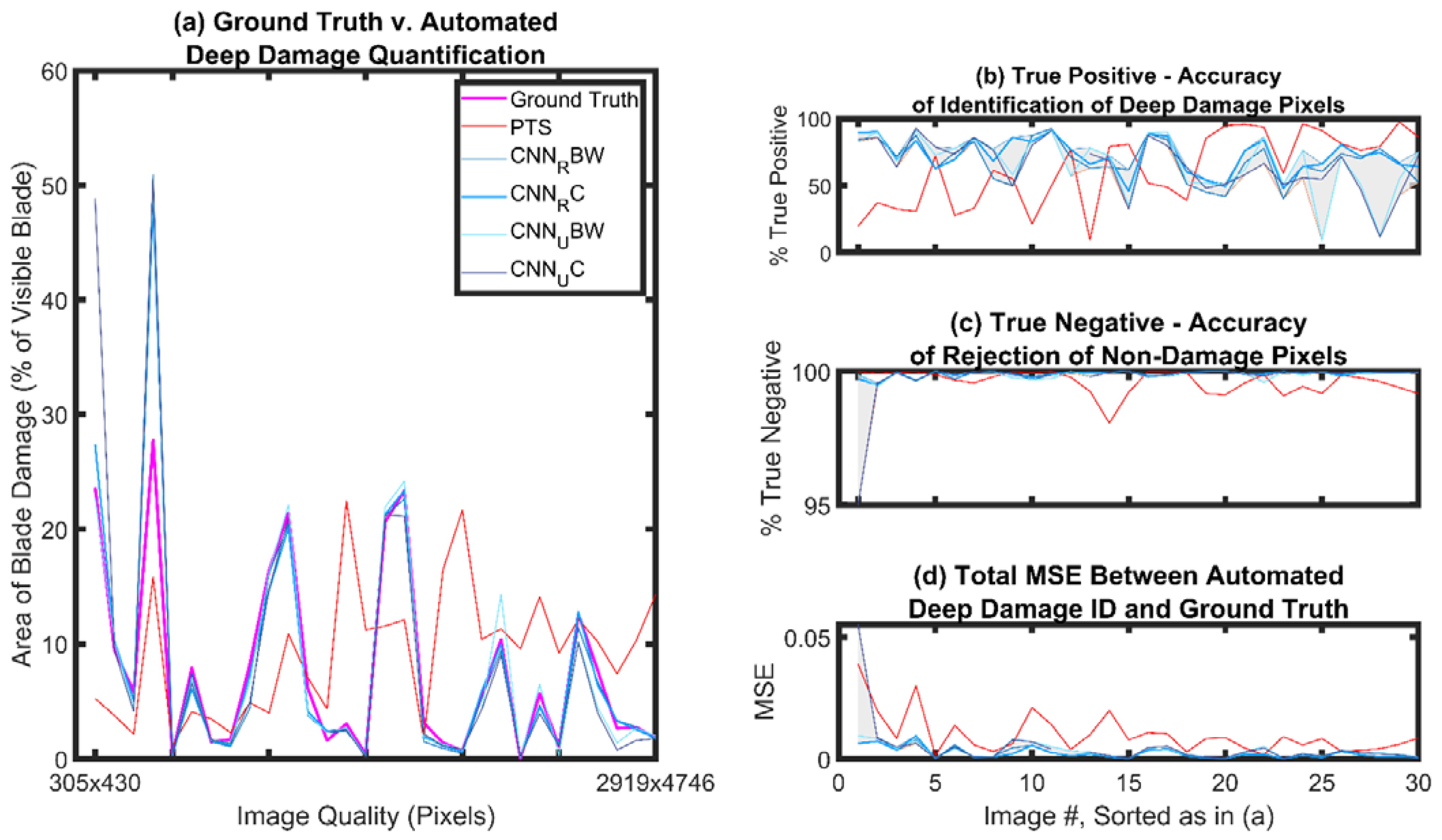
Results for deep damage detection are presented in Table 5 and indicate the unsupervised PTS model identifies a mean of 62.1% of deep damage pixels per image (averaged over all test images) (Figure 12b). The PTS module correctly identifies 99.6% of pixels that do not exhibit deep damage (Figure 12c). The mean percent area of deep LEE over the 30 testing images in the ground-truth analysis is 7.8% of the visible blade area while the mean automatically detected deep LEE area from the PTS module is 9.2% (Figure 12a). For the highest performing CNN, C N N R C , the mean area of the blade with deep damage over the 30 test images is 8.2%. However, as previously discussed, all four CNN models generally resolve the percent LEE better on a per image basis when compared to the PTS module (Figure 12a).
The PTS detection of deep damage is notably better than that for all damage (i.e., from the PTS damage proposal model). This is likely due to the implementation of three clusters when classifying LEE within the PTS module, which allows for reduction of noise and refinement of damage identification. This is also evident in the increase in true negatives observed for the PTS deep damage classification (Figure 12c).
The CNN with the highest accuracy in identifying deep LEE pixels is C N N R C with a mean of 72.5% true positives per image (Figure 12b). Poorest performance is found for C N N U C , (65.5% of deep damage pixels are correctly identified). Mean CNN accuracy (averaged over all four CNNs) in identifying pixels with deep damage is 68.25%. This is a notable increase in accuracy compared to the total damage proposal results for the CNNs. This can be attributed to the inherent difficulty in identification of shallow versus deep damage. Deep damage is generally much more spatially coherent and extensive than shallow damage and has a lower dispersion of pixel intensities (Figure 2 and Figure 5). Thus, when considering only deep damage, accuracy increases both in terms of true positives and true negatives.
The ground-truth estimate of shallow damage (derived using visual inspection of the images) averaged over all 30 testing images is 1.2% of the visible blade area, while the mean automatically detected shallow damage from the PTS module is 1.7% (Figure 13a). However, the pixel-by-pixel assessment indicates that PTS accurately identified only 6.6% of pixels that have shallow damage according to the visual inspection analysis (Table 5, Figure 13b). PTS correctly identifies 99.8% of True Negatives per image (Figure 13c). This damage class is much more difficult to detect than deep damage, yet early detection of shallow LEE is important for preventing continuation and evolution of damage. Thus, the technique may provide (1) indication of whether there is shallow damage present in a field image and (2) estimate of the area of LEE present within the dataset as a whole. Further, the MSE of the PTS classification module decreases markedly with image quality, and the results exhibit lower dispersion relative to subjective annotation (Figure 13c).
The CNN with the highest (lowest) accuracy in identifying pixels with shallow damage is C N N U B W ( C N N R C ) with a mean true positive of 28.5% (24.5%) of shallow LEE pixels accurately identified per image (Figure 13b). For the highest performing CNN, C N N U B W , the mean detected percent area of shallow LEE over the 30 testing images is 1.0% of the visible blade area (Figure 13a). Interestingly, the CNN trained and tested on unrotated, black and white images performs best for this task ( C N N U B W ) compared to the better performance of C N N R C in detection of deep damage. This may indicate that characteristics of the shallow class pertaining to color and hue are less important than shape or texture when considering CNN detection.
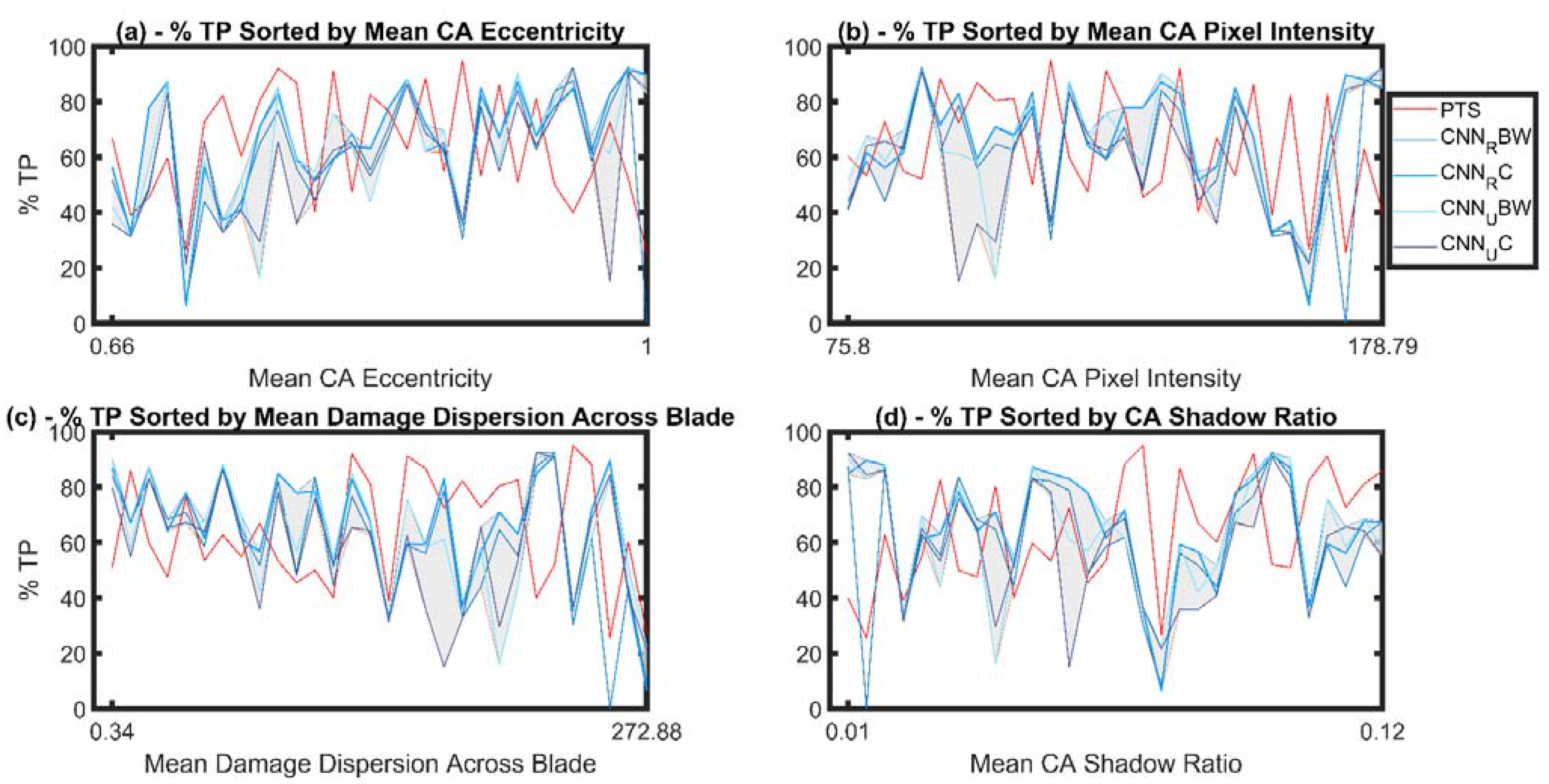
Damage dispersion across the blade is measured using the mean Euclidean distance from the centroid of a given LEE CA to the centroid of its nearest LEE CA and thus describes how scattered the damage is for a given image. When the accuracy of LEE quantification (expressed as percent true positive (TP) LEE pixel identifications) are conditioned on per-image damage dispersion across the blade, the results show accuracy for both the PTS and CNN methods decreases with increasing damage dispersion along the blade (Figure 14c). In other words, for images in which the damage is not closely clustered, both methods exhibit lower success in LEE identification. This is also evident in examples of model output in Figure 8, Figure 9 and Figure 10; both methods are more consistent for blade damage that is uniform and continuous along the blade versus for damage that is more fragmented.
CNN results improve with increased CA eccentricity (Figure 14a); this may be due in part to the higher eccentricity and damage coherence associated with the deep damage class, which the CNNs exhibit higher skill in identifying (Figure 5, Figure 12 and Figure 14). Further, accuracy for both methods decreases with increases in pixel intensity, which is reflective of the higher pixel intensities associated with the shallow damage class and the lower accuracy of both methods for identifying shallow damage (Figure 5, Figure 13 and Figure 14). PTS LEE detection accuracy generally increases with increases in per-image mean CA shadow ratio. The deep damage class is generally associated with lower mean CA shadow ratio (Figure 5), further confirming the findings that the PTS method is more skilled for precise identification of deep damage than shallow damage (Figure 12 and Figure 13).

4. Discussion and Conclusions

Although a range of advanced structural and condition monitoring techniques are being developed and applied to wind turbine blades, image processing techniques remain at the core of efforts to provide early guidance on the presence and progression of leading edge erosion. However, the optimal method to apply to identify and characterize damage remains uncertain. Here, two machine learning models are developed, applied and evaluated for automated wind turbine blade leading edge erosion (LEE) quantification and classification in field images. One model (PTS—pixel intensity and adaptive thresholding with shadow ratio) uses unsupervised learning methods (primarily k-means segmentation) with a combination of optimized preprocessing and image thresholding parameters. The second model is a supervised, region-based convolutional neural network (CNN). Both models aim to automatically quantify (return the percent area of the visible blade area that exhibits damage) and classify (deep, shallow) damage within the images.
A dataset of 140 field images of wind turbine blades exhibiting varying severity of LEE is used to develop, optimize, and test the models. The field images exhibit variations in lighting and shadow conditions, orientation of the blade within the image, image quality (resolution), and the presence/absence of other components (i.e., cloud/ground/tower). All types of leading edge erosion are represented in the dataset, including pitting and marring (shallow, surface-level perforations (pitting) and scratches (marring), along the leading edge that do not reveal underlying blade material), and gouges and delamination (deep damage instances that are concentrated (gouges) or expansive (delamination) and damage the blade coating, revealing underlying material). The dataset contains approximately 2300 and 1200 unique instances of shallow and deep damage, respectively. Images are subjectively annotated for deep and shallow damage classes, and these annotations are used to train and test the supervised models and in testing of the unsupervised models.
In the first step, the pixels representing the visible blade area are distinguished from the background. The mean true positive of 93.7% indicates an average of 93.7% of ground truth blade pixels are correctly identified per image. Results for damage quantification are promising for both methods, with both supervised and unsupervised methods correctly identifying approximately 65% of total damage pixels in the testing dataset when compared to subjective annotation. Further, both methods exhibit low rates of false positives for damage identification, with approximately 99% of non-damage pixels correctly rejected. Both methods exhibit similar success rates when identifying pixels within the deep LEE class, with the CNN identifying 68% of deep damage pixels compared to 62% for the PTS method. Both methods again exhibit low rates of false positives for damage classification, with approximately 99% of non-deep LEE pixels correctly rejected. The shallow damage class, which generally exhibits more variations in mean pixel intensity, shape, and a much smaller average area than deep damage, is more difficult for both methods to detect. The CNN method detects approximately 28% of shallow damage pixels, while the PTS method detects approximately 5% of shallow damage pixels. However, for both methods, returned estimates for the percent blade area encompassed by shallow LEE exhibit a percent difference of only 20 and 30% for the PTS and CNN methods, respectively. Further, both methods exhibit low rates of false positives for shallow damage identification, with 99% of non-shallow LEE pixels correctly rejected. Further work is needed to fully address the difficulty in identifying nascent (shallow) damage, but skill is strongly manifest for damage regimes of critical importance to wind farm owner-operators. Rotation of the images to ensure a common blade orientation enhances the ability of the CNN to detect damage but conversion of black and white images does not greatly impact damage detection fidelity.
Other techniques are being advanced to quantify and characterize damage on wind turbine blades including, for example, active thermography [74]. The techniques described herein are designed to be applied to images in the visual portion of the radiation spectrum but naturally could also be adapted to work with other types of images. The PTS and CNN techniques presented herein show promise when applied to field inspection images, are rapid to apply, objective and can be readily applied to the vast number of field inspection images that exist within the wind energy industry to retrospectively assess damage progression. They could also be used to classify blade erosion in images from laboratory experiments (e.g., whirling arm rig experiments) where fewer technical challenges regarding lighting variability and screen capture regimes would undoubtedly benefit accuracy. The methods may be improved through refining training parameters via introduction of larger datasets.

Author Contributions

Conceptualization, R.J.B. and S.C.P.; methodology, J.A.A. and R.J.B.; formal analysis, J.A.A.; writing—review and editing, J.A.A., R.J.B. and S.C.P. All authors have read and agreed to the published version of the manuscript.

Funding

S.C.P. is funded by the U.S. Department of Energy via a subcontract to Sandia National Laboratory. Computational resources to S.C.P. used in these analyses are provided by the NSF Extreme Science and Engineering Discovery Environment (XSEDE and XSEDE2) (award TG-ATM170024). R.J.B. was funded by US Department of Energy (DE-SC0016438). J.A.A. is funded by the NSF GRFP (DGE-1650441).

Data Availability Statement

The image sets used in this research are confidential and cannot be provided.

Acknowledgments

We acknowledge with gratitude the confidential provision of the blade leading erosion images.

Conflicts of Interest

The authors declare no conflict of interest.

References

  1. Wiser, R.; Bolinger, M.; Hoen, B.; Millstein, D.; Rand, J.; Barbose, G.; Darghouth, N.; Gorman, W.; Jeong, S.; Paulos, B. Land-Based Wind Market Report: 2022 Edition; Lawrence Berkeley National Lab: Berkeley, CA, USA, 2022. [Google Scholar]
  2. Barthelmie, R.J.; Shepherd, T.J.; Aird, J.A.; Pryor, S.C. Power and wind shear implications of large wind turbine scenarios in the US Central Plains. Energies 2020, 13, 4269. [Google Scholar] [CrossRef]
  3. Musial, W.; Spitsen, P.; Duffy, P.; Beiter, P.; Marquis, M.; Hammond, R.; Shields, M. Offshore Wind Market Report: 2022 Edition; (No. NREL/TP-5000-83544); National Renewable Energy Lab: Golden, CO, USA, 2022.
  4. Alsaleh, A.; Sattler, M. Comprehensive life cycle assessment of large wind turbines in the US. Clean Technol. Environ. Policy 2019, 21, 887–903. [Google Scholar] [CrossRef]
  5. Du, Y.; Zhou, S.; Jing, X.; Peng, Y.; Wu, H.; Kwok, N. Damage detection techniques for wind turbine blades: A review. Mech. Syst. Signal Process 2020, 141, 106445. [Google Scholar] [CrossRef]
  6. Pryor, S.C.; Barthelmie, R.J.; Cadence, J.; Dellwik, E.; Hasager, C.B.; Kral, S.T.; Reuder, J.; Rodgers, M.; Veraart, M. Atmospheric Drivers of Wind Turbine Blade Leading Edge Erosion: Review and Recommendations for Future Research. Energies 2022, 15, 8553. [Google Scholar] [CrossRef]
  7. Mishnaevsky, L., Jr.; Hasager, C.B.; Bak, C.; Tilg, A.M.; Bech, J.I.; Rad, S.D.; Fæster, S. Leading edge erosion of wind turbine blades: Understanding, prevention and protection. Renew. Energy 2021, 169, 953–969. [Google Scholar] [CrossRef]
  8. Herring, R.; Dyer, K.; Martin, F.; Ward, C. The increasing importance of leading edge erosion and a review of existing protection solutions. Renew. Sustain. Energy Rev. 2019, 115, 109382. [Google Scholar] [CrossRef]
  9. Mishnaevsky, L., Jr.; Thomsen, K. Costs of repair of wind turbine blades: Influence of technology aspects. Wind. Energy 2020, 23, 2247–2255. [Google Scholar] [CrossRef]
  10. Ravishankara, A.K.; Özdemir, H.; Van der Weide, E. Analysis of leading edge erosion effects on turbulent flow over airfoils. Renew. Energy 2021, 172, 765–779. [Google Scholar] [CrossRef]
  11. Amirzadeh, B.; Louhghalam, A.; Raessi, M.; Tootkaboni, M. A computational framework for the analysis of rain-induced erosion in wind turbine blades, part I: Stochastic rain texture model and drop impact simulations. J. Wind Eng. Ind. Aerodyn. 2017, 163, 33–43. [Google Scholar] [CrossRef] [Green Version]
  12. Fraisse, A.; Bech, J.I.; Borum, K.K.; Fedorov, V.; Johansen NF, J.; McGugan, M.; Mishnaevsky, L., Jr.; Kusano, Y. Impact fatigue damage of coated glass fibre reinforced polymer laminate. Renew. Energy 2018, 126, 1102–1112. [Google Scholar] [CrossRef] [Green Version]
  13. Carraro, M.; De Vanna, F.; Zweiri, F.; Benini, E.; Heidari, A.; Hadavinia, H. CFD modeling of wind turbine blades with eroded leading edge. Fluids 2022, 7, 302. [Google Scholar] [CrossRef]
  14. Han, W.; Kim, J.; Kim, B. Effects of contamination and erosion at the leading edge of blade tip airfoils on the annual energy production of wind turbines. Renew. Energy 2018, 115, 817–823. [Google Scholar] [CrossRef]
  15. Schramm, M.; Rahimi, H.; Stoevesandt, B.; Tangager, K. The influence of eroded blades on wind turbine performance using numerical simulations. Energies 2017, 10, 1420. [Google Scholar] [CrossRef] [Green Version]
  16. Papi, F.; Cappugi, L.; Salvadori, S.; Carnevale, M.; Bianchini, A. Uncertainty quantification of the effects of blade damage on the actual energy production of modern wind turbines. Energies 2020, 13, 3785. [Google Scholar] [CrossRef]
  17. Gaudern, N. A practical study of the aerodynamic impact of wind turbine blade leading edge erosion. J. Phys. Conf. Ser. 2014, 524, 012031. [Google Scholar] [CrossRef]
  18. Letson, F.; Shepherd, T.J.; Barthelmie, R.J.; Pryor, S.C. WRF modeling of deep convection and hail for wind power applications. J. Appl. Meteorol. Climatol. 2020, 59, 1717–1733. [Google Scholar] [CrossRef]
  19. Verma, A.S.; Castro, S.G.; Jiang, Z.; Teuwen, J.J. Numerical investigation of rain droplet impact on offshore wind turbine blades under different rainfall conditions: A parametric study. Compos. Struct. 2020, 241, 112096. [Google Scholar] [CrossRef]
  20. Knobbe-Eschen, H.; Stemberg, J.; Abdellaoui, K.; Altmikus, A.; Knop, I.; Bansmer, S.; Balaresque, N.; Suhr, J. Numerical and experimental investigations of wind-turbine blade aerodynamics in the presence of ice accretion. In Proceedings of the AIAA Scitech 2019 Forum, San Diego, CA, USA, 7–11 January 2019; p. 0805. [Google Scholar]
  21. Lau, B.C.P.; Ma, E.W.M.; Pecht, M. Review of offshore wind turbine failures and fault prognostic methods. In Proceedings of the IEEE 2012 Prognostics and System Health Management Conference, Beijing, China, 23–25 May 2012; pp. 1–5. [Google Scholar]
  22. Wood, R.J.; Lu, P. Leading edge topography of blades—A critical review. Surf. Topogr. 2021, 9, 023001. [Google Scholar] [CrossRef]
  23. Slot, H.M.; Gelinck, E.R.M.; Rentrop, C.; Van Der Heide, E. Leading edge erosion of coated wind turbine blades: Review of coating life models. Renew. Energy 2015, 80, 837–848. [Google Scholar] [CrossRef]
  24. Springer, G.S.; Yang, C.I.; Larsen, P.S. Analysis of rain erosion of coated materials. J. Compos. Mater. 1974, 8, 229–252. [Google Scholar] [CrossRef]
  25. Pryor, S.C.; Letson, F.W.; Shepherd, T.J.; Barthelmie, R.J. Evaluation of WRF simulation of deep convection in the US Southern Great Plains. J. Appl. Meteorol. Climatol. 2023, 62, 41–62. [Google Scholar] [CrossRef]
  26. Letson, F.; Barthelmie, R.J.; Pryor, S.C. Radar-derived precipitation climatology for wind turbine blade leading edge erosion. Wind Energy Sci. 2020, 5, 331–347. [Google Scholar] [CrossRef] [Green Version]
  27. Keegan, M.H. Wind Turbine Blade Leading Edge Erosion, an Investigation of Rain Droplet and Hailstone Impact Induced Damage Mechanisms. Ph.D. Thesis, University of Strathclyde, Glasgow, UK, 2014. [Google Scholar]
  28. Springer, G.S. Erosion by Liquid Impact; Springer: Berlin, Germany, 1976. [Google Scholar]
  29. Castorrini, A.; Venturini, P.; Corsini, A.; Rispoli, F. Machine learnt prediction method for rain erosion damage on wind turbine blades. Wind Energy 2021, 24, 917–934. [Google Scholar] [CrossRef]
  30. Hoksbergen, N.; Akkerman, R.; Baran, I. The Springer model for lifetime prediction of wind turbine blade leading edge protection systems: A review and sensitivity study. Materials 2022, 15, 1170. [Google Scholar] [CrossRef]
  31. Eisenberg, D.; Laustsen, S.; Stege, J. Wind turbine blade coating leading edge rain erosion model: Development and validation. Wind Energy 2018, 21, 942–951. [Google Scholar] [CrossRef]
  32. Hoksbergen, T.H.; Baran, I.; Akkerman, R. Rain droplet erosion behavior of a thermoplastic based leading edge protection system for wind turbine blades. IOP Conf. Ser. Mater. Sci. Eng. 2020, 942, 012023. [Google Scholar] [CrossRef]
  33. Tobin, E.F.; Young, T.M. Analysis of incubation period versus surface topographical parameters in liquid droplet erosion tests. Mater. Perform. Charact. 2017, 6, 144–164. [Google Scholar] [CrossRef]
  34. McGugan, M.; Mishnaevsky, L., Jr. Damage mechanism based approach to the structural health monitoring of wind turbine blades. Coatings 2020, 10, 1223. [Google Scholar] [CrossRef]
  35. Stephenson, S. Wind blade repair: Planning, safety, flexibility. Composites World, 1 August 2011. [Google Scholar]
  36. Major, D.; Palacios, J.; Maughmer, M.; Schmitz, S. Aerodynamics of leading-edge protection tapes for wind turbine blades. Wind Eng. 2021, 45, 1296–1316. [Google Scholar] [CrossRef]
  37. Bech, J.I.; Hasager, C.B.; Bak, C. Extending the life of wind turbine blade leading edges by reducing the tip speed during extreme precipitation events. Wind Energy Sci. 2018, 3, 729–748. [Google Scholar] [CrossRef] [Green Version]
  38. Rempel, L. Rotor blade leading edge erosion-real life experiences. Wind. Syst. Mag. 2012, 11, 22–24. [Google Scholar]
  39. Amirat, Y.; Benbouzid, M.E.H.; Al-Ahmar, E.; Bensaker, B.; Turri, S. A brief status on condition monitoring and fault diagnosis in wind energy conversion systems. Renew. Sustain. Energy Rev. 2009, 13, 2629–2636. [Google Scholar] [CrossRef] [Green Version]
  40. Yan, Y.J.; Cheng, L.; Wu, Z.Y.; Yam, L.H. Development in vibration-based structural damage detection technique. Mech. Syst. Signal Process. 2007, 21, 2198–2211. [Google Scholar] [CrossRef]
  41. Juengert, A.; Grosse, C.U. Inspection techniques for wind turbine blades using ultrasound and sound waves. In Proceedings of the NDTCE, Nantes, France, 30 June–3 July 2009; Volume 9. [Google Scholar]
  42. Van Dam, J.; Bond, L.J. Acoustic emission monitoring of wind turbine blades. Smart Mater. Non-Destr. Eval. Energy Syst. 2015, 9439, 55–69. [Google Scholar]
  43. Xu, D.; Wen, C.; Liu, J. Wind turbine blade surface inspection based on deep learning and UAV-taken images. J. Renew. Sustain. Energy 2019, 11, 053305. [Google Scholar] [CrossRef]
  44. Sørensen, B.F.; Lading, L.; Sendrup, P. Fundamentals for Remote Structural Health Monitoring of Wind Turbine Blades-A Pre-Project; U.S. Department of Energy: Washington, DC, USA, 2002.
  45. Shihavuddin, A.S.M.; Chen, X.; Fedorov, V.; Nymark Christensen, A.; Andre Brogaard Riis, N.; Branner, K.; Bjorholm Dahl, A.; Reinhold Paulsen, R. Wind turbine surface damage detection by deep learning aided drone inspection analysis. Energies 2019, 12, 676. [Google Scholar] [CrossRef] [Green Version]
  46. Yu, Y.; Cao, H.; Liu, S.; Yang, S.; Bai, R. Image-based damage recognition of wind turbine blades. In Proceedings of the 2017 2nd International Conference on Advanced Robotics and Mechatronics (ICARM), Hefei and Tai’an, China, 27–31 August 2017; pp. 161–166. [Google Scholar]
  47. Yang, P.; Dong, C.; Zhao, X.; Chen, X. The surface damage identifications of wind turbine blades based on ResNet50 algorithm. In Proceedings of the 2020 39th Chinese Control Conference (CCC), Shenyang, China, 27–30 July 2020; pp. 6340–6344. [Google Scholar]
  48. Bradley, D.; Roth, G. Adaptive thresholding using the integral image. J. Graph. Tools 2007, 12, 13–21. [Google Scholar] [CrossRef]
  49. Zulpe, N.; Pawar, V. GLCM textural features for brain tumor classification. Int. J. Comput. Sci. Issues 2012, 9, 354. [Google Scholar]
  50. Sirmacek, B.; Unsalan, C. Damaged building detection in aerial images using shadow information. In Proceedings of the 2009 4th International Conference on Recent Advances in Space Technologies, Istanbul, Turkey, 11–13 June 2009; pp. 249–252. [Google Scholar]
  51. Unsalan, C.; Boyer, K.L. Linearized vegetation indices based on a formal statistical framework. IEEE Trans. Geosci. Remote Sens. 2004, 42, 1575–1585. [Google Scholar] [CrossRef]
  52. Maniaci, D.C.; MacDonald, H.; Paquette, J.; Clarke, R. Leading Edge Erosion Classification System; Technical Report from IEA Wind Task 46 Erosion of Wind Turbine Blades; Technical University of Denmark: Lyngby, Denmark, 2022; 52p. [Google Scholar]
  53. Wang, Y.; Hu, R.; Zheng, X. Aerodynamic analysis of an airfoil with leading edge pitting erosion. J. Sol. Energy Eng. 2017, 139, 061002. [Google Scholar] [CrossRef]
  54. Sareen, A.; Sapre, C.A.; Selig, M.S. Effects of leading edge erosion on wind turbine blade performance. Wind. Energy 2014, 17, 1531–1542. [Google Scholar] [CrossRef]
  55. Mishnaevsky, L., Jr. Root causes and mechanisms of failure of wind turbine blades: Overview. Materials 2022, 15, 2959. [Google Scholar] [CrossRef] [PubMed]
  56. McGugan, M.; Pereira, G.; Sørensen, B.F.; Toftegaard, H.; Branner, K. Damage tolerance and structural monitoring for wind turbine blades. Philos. Trans. R. Soc. A Math. Phys. Eng. Sci. 2015, 373, 20140077. [Google Scholar] [CrossRef]
  57. Peacock, J.A. Two-dimensional goodness-of-fit testing in astronomy. Mon. Notices Royal Astron. Soc. 1983, 202, 615–627. [Google Scholar] [CrossRef] [Green Version]
  58. Alloghani, M.; Al-Jumeily, D.; Mustafina, J.; Hussain, A.; Aljaaf, A.J. A systematic review on supervised and unsupervised machine learning algorithms for data science. In Supervised and Unsupervised Learning for Data Science. Unsupervised and Semi-Supervised Learning; Berry, M., Mohamed, A., Yap, B., Eds.; Springer: Cham, Switzerland, 2020; pp. 3–21. [Google Scholar]
  59. Zheng, X.; Lei, Q.; Yao, R.; Gong, Y.; Yin, Q. Image segmentation based on adaptive K-means algorithm. EURASIP J. Image Video Process. 2018, 2018, 1–10. [Google Scholar] [CrossRef]
  60. Burney, S.A.; Tariq, H. K-means cluster analysis for image segmentation. Int. J. Comput. Appl. 2014, 96, 872–878. [Google Scholar]
  61. Maddern, W.; Stewart, A.; McManus, C.; Upcroft, B.; Churchill, W.; Newman, P. Illumination invariant imaging: Applications in robust vision-based localisation, mapping and classification for autonomous vehicles. In Proceedings of the Visual Place Recognition in Changing Environments Workshop, IEEE International Conference on Robotics and Automation (ICRA), Hong Kong, China, 31 May–7 June 2014; Volume 2, p. 5. [Google Scholar]
  62. Sharma, G.; Wu, W.; Dalal, E.N. The CIEDE2000 Color-Difference Formula: Implementation Notes, Supplementary Test Data, and Mathematical Observations. Color Res. Appl. 2005, 30, 21–30. [Google Scholar] [CrossRef]
  63. Chaki, N.; Shaikh, S.H.; Saeed, K.; Chaki, N.; Shaikh, S.H.; Saeed, K. A Comprehensive Survey on Image Binarization Techniques; Springer: New Delhi, India, 2014; pp. 5–15. [Google Scholar]
  64. Rawat, W.; Wang, Z. Deep convolutional neural networks for image classification: A comprehensive review. Neural Comput. 2017, 29, 2352–2449. [Google Scholar] [CrossRef]
  65. Hu, G.; Yang, Y.; Yi, D.; Kittler, J.; Christmas, W.; Li, S.Z.; Hospedales, T. When face recognition meets with deep learning: An evaluation of convolutional neural networks for face recognition. In Proceedings of the IEEE International Conference on Computer Vision Workshops, Santiago, Chile, 7–13 December 2015; pp. 142–150. [Google Scholar]
  66. Dhillon, A.; Verma, G.K. Convolutional neural network: A review of models, methodologies and applications to object detection. Prog. Artif. Intell. 2020, 9, 85–112. [Google Scholar] [CrossRef]
  67. Hossain, T.; Shishir, F.S.; Ashraf, M.; Al Nasim, M.A.; Shah, F.M. Brain tumor detection using convolutional neural network. In Proceedings of the 2019 1st International Conference on Advances in Science, Engineering and Robotics Technology, Dhaka, Bangladesh, 3–5 May 2019; pp. 1–6. [Google Scholar]
  68. Aird, J.A.; Quon, E.W.; Barthelmie, R.J.; Debnath, M.; Doubrawa, P.; Pryor, S.C. Region-based convolutional neural network for wind turbine wake characterization in complex terrain. Remote Sens. 2021, 13, 4438. [Google Scholar] [CrossRef]
  69. Aird, J.A.; Quon, E.W.; Barthelmie, R.J.; Pryor, S.C. Region-based convolutional neural network for wind turbine wake characterization from scanning lidars. J. Phys. Conf. Ser. 2022, 2265, 032077. [Google Scholar] [CrossRef]
  70. Guo, W.; Yang, W.; Zhang, H.; Hua, G. Geospatial object detection in high resolution satellite images based on multi-scale convolutional neural network. Remote Sens. 2018, 10, 131. [Google Scholar] [CrossRef] [Green Version]
  71. He, K.; Gkioxari, G.; Dollár, P.; Girshick, R. Mask r-cnn. In Proceedings of the IEEE International Conference on Computer Vision, Venice, Italy, 22–29 October 2017; pp. 2961–2969. [Google Scholar]
  72. Badilla-Solórzano, J.; Spindeldreier, S.; Ihler, S.; Gellrich, N.C.; Spalthoff, S. Deep-learning-based instrument detection for intra-operative robotic assistance. Int. J. Comput. Assist. Radiol. Surg. 2022, 17, 1685–1695. [Google Scholar] [CrossRef] [PubMed]
  73. Lin, T.Y.; Dollár, P.; Girshick, R.; He, K.; Hariharan, B.; Belongie, S. Feature pyramid networks for object detection. In Proceedings of the IEEE Conference on Computer Vision and Pattern Recognition, Honolulu, HI, USA, 21–26 July 2017; pp. 2117–2125. [Google Scholar]
  74. Jensen, F.; Jerg, J.F.; Sorg, M.; Fischer, A. Active thermography for the interpretation and detection of rain erosion damage evolution on GFRP airfoils. NDT E Int. 2023, 135, 102778. [Google Scholar] [CrossRef]
Figure 1. Example of a field image containing extensive LEE of varying severity. All damage in the dataset is classified as either deep (delamination/gouges—continuous/concentrated damage that removes the outer laminate layer, revealing internal material) or shallow (pits/marring—concentrated/continuous damage to the laminate layer that does not reveal internal material).
Energies 16 02820 g001
Figure 2. Empirical cumulative density functions (CDFs) of the 140 images in terms of: (a) the fraction of the blade area that exhibits shallow (green) and deep (magenta) LEE, (b) the number of discrete instances of shallow and deep LEE, (c) orientation of the leading edge within the image (where 0° indicates the blade is horizontally aligned within the image), (d) blade resolution, defined as the number of pixels in each image that contain the blade.
Energies 16 02820 g002
Figure 3. Flowchart of entire LEE quantification model development and testing process showing the common aspects; image preprocessing and blade area quantification (purple) and the subsequent separation into the unsupervised (PTS—red)/supervised (CNN—blue) methods.
Energies 16 02820 g003
Figure 4. Workflow of the unsupervised LEE quantification (PTS—pixel intensity threshold and shadow ratio) module 2.
Energies 16 02820 g004
Figure 5. Empirical CDFs comparing dataset-wide (i.e., all images including testing, training, and validation subsets) variations in deep and shallow damage characteristics: (a) eccentricity, (b) pixel intensity, (c) shadow ratio. Shallow and deep damage CDFs are constructed using statistics from each unique damage instance (CA) across all images in the dataset, i.e., the number of CDF datapoints is equal to the number of instances of shallow and deep damage across all images.
Energies 16 02820 g005
Figure 6. Example image (a) and CNN annotations (b) used to train the supervised learning damage detection model. Coherence areas with shallow damage are outlined in red, while coherent areas with deep damage are outlined in green.
Energies 16 02820 g006
Figure 7. (a) Automated blade area quantification algorithm results (purple) compared to subjective (ground-truth) blade area (magenta). (b) Accuracy of automated identification of blade pixels compared to the ground-truth. (c) Accuracy of rejection of non-blade pixels compared to subjective identification (higher accuracy denotes fewer false positives in pixels assigned to the blade class, i.e., less noise). (d) Total mean square error between automated and subjective blade pixel identification.
Energies 16 02820 g007
Figure 8. Example (a) field image and output of automated (c) PTS and (d) CNN LEE quantification and classification for shallow (green) and deep (magenta) LEE compared to (b) ground-truth LEE quantification and classification.
Energies 16 02820 g008
Figure 9. Example (a) field image and output of automated (c) PTS and (d) CNN LEE quantification and classification for shallow (green) and deep (magenta) LEE compared to (b) ground-truth LEE quantification and classification.
Energies 16 02820 g009
Figure 10. Example (a) field image and output of automated (c) PTS and (d) CNN LEE quantification and classification for shallow (green) and deep (magenta) LEE compared to (b) ground-truth LEE quantification and classification.
Energies 16 02820 g010
Figure 11. (a) Automated LEE quantification results for the unsupervised PTS module (red) and supervised CNN modules (blue) compared to subjective quantification for all damage (deep and shallow) (magenta). (b) Accuracy of automated identification of LEE pixels compared to subjective identification. (c) Accuracy of rejection of non-LEE pixels compared to subjective identification (higher accuracy denotes fewer false positives in pixels assigned to the LEE class, i.e., less noise). (d) Total mean square error between automated and subjective LEE pixel identification. The gray shading shows the dispersion in the CNN results (maximum and minimum CNN results for each panel, i.e. b, c, and d, are used as the boundaries for the gray shading).
Energies 16 02820 g011
Figure 12. (a) Automated deep LEE quantification results for the unsupervised PTS module (red) and supervised CNN modules (blue) compared to subjective quantification for deep damage (magenta). (b) Accuracy of automated identification of deep LEE pixels compared to subjective identification. (c) Accuracy of rejection of non-LEE pixels compared to subjective identification (higher accuracy denotes fewer false positives in pixels assigned to the deep LEE class, i.e., less noise). (d) Total mean square error between automated and subjective deep LEE pixel identification. The gray shading shows the dispersion in the CNN results (maximum and minimum CNN results for each panel, i.e., b, c, and d, are used as the boundaries for the gray shading).
Energies 16 02820 g012
Figure 13. (a) Automated shallow LEE quantification results for the unsupervised PTS module (red) and supervised CNN modules (blue) compared to subjective quantification for shallow damage (magenta). (b) Accuracy of automated identification of shallow LEE pixels compared to subjective identification. (c) Accuracy of rejection of non-LEE pixels compared to subjective identification (higher accuracy denotes fewer false positives in pixels assigned to the shallow LEE class, i.e., less noise). (d) Total mean square error between automated and subjective shallow LEE pixel identification.
Energies 16 02820 g013
Figure 14. Damage quantification results for unsupervised (PTS) and supervised (CNN) models, shown as the percent of pixels accurately identified as damage when compared to subjective identification (% true positive (TP)). For each panel, quantification results are sorted in ascending order in terms of per-image mean (a) CA eccentricity, (b) CA pixel intensity, (c) damage dispersion across the blade, and (d) CA shadow ratio. Gray shading is applied to show the dispersion between CNN % TP values for each image. The gray shading shows the dispersion in the CNN results (maximum and minimum CNN results for each panel, i.e. b, c, and d, are used as the boundaries for the gray shading).
Energies 16 02820 g014
Table 1. Image preprocessing parameters used in the MATLAB (R2021a) image toolbox (Matlab functions utilized are imflatfield ( σ ) , localcontrast (E); saturation is enhanced via augmenting the saturation values in the hsv colorspace by a value of C). These preprocessing steps are found to enhance unsupervised model accuracy and are optimized for application to field images of wind turbine blades. The parameters may be adjusted and optimized for other automated LEE quantification applications, such as for use in a whirling arm study.
ParameterUsageModule (See Figure 3)Value
ELocal contrast operation to enhance edges within the image1—Blade Area Quantification
2—PTS damage proposal
3—PTS damage classification
0.2
CChroma alteration; image saturation is enhanced 1—Blade Area Quantification,
2—PTS damage proposal
3—PTS damage classification
0.5
σ Flat-field correction; Gaussian smoothing with a standard deviation of σ is utilized to correct image shading distortion2—PTS damage proposal8
Table 2. Final optimized image thresholding parameters for the PTS damage proposal module (optimized by minimizing MSE—see Equation (1)).
ParameterUsageValue
QShadow ratio quantile0.009
S A T Adjusts sensitivity of adaptive thresholding to luminance of foreground/background pixels (the damage is often distinguished as background pixels due to associated lower pixel intensity).0.3
Table 3. Final optimized parameters for training each Mask R-CNN model for LEE quantification and classification.
ParameterUsageValue
Learning RateSpecifies the pace at which the machine learning model learns the input data0.001
Batch SizeNumber of training examples in one iteration 2
EpochsNumber of times the CNN processes the entire dataset during training225
Table 4. Configurations for Mask R-CNN sensitivity study.
Image rotated by α L E to ensure the blade is horizontal in the imageUnrotated Image
Black and White C N N R B W C N N U B W
Color C N N R C C N N U C
Table 5. Accuracy of the three tasks (blade area quantification, damage quantification, damage classification) for each method.
TaskModelAccuracy (% of Pixels Correctly Identified Relative to Ground Truth)
Blade Area QuantificationModule 193.7
Damage QuantificationPTS (Module 2)63.9
CNN61.4 (mean CNN), [58.1, 65.9] [min = C N N U C , max = C N N R C ]
Deep Damage ClassificationPTS (Module 3)62.1
CNN68.3 (mean CNN), [65.5, 72.5] [min = C N N U C , max = C N N R C ]
Shallow Damage ClassificationPTS (Module 3)6.6
CNN26.1 (mean CNN), [24.5, 28.5] [min = C N N R C , max = C N N U B W ]
Disclaimer/Publisher’s Note: The statements, opinions and data contained in all publications are solely those of the individual author(s) and contributor(s) and not of MDPI and/or the editor(s). MDPI and/or the editor(s) disclaim responsibility for any injury to people or property resulting from any ideas, methods, instructions or products referred to in the content.