Review

A Comprehensive Examination of Vector-Controlled Induction Motor Drive Techniques

by
Ahmed G. Mahmoud A. Aziz
1,2,
Almoataz Y. Abdelaziz
3,*,
Ziad M. Ali
4,5 and
Ahmed A. Zaki Diab
1,*
1
Electrical Engineering Department, Faculty of Engineering, Minia University, Minia 61111, Egypt
2
Electrical and Computer Department, Higher Institute of Engineering and Technology New El Minia, Minia 61111, Egypt
3
Faculty of Engineering & Technology, Future University in Egypt, Cairo 11835, Egypt
4
College of Engineering at Wadi Addawasir, Prince Sattam bin Abdulaziz University, Wadi Addawasir 11991, Saudi Arabia
5
Electrical Engineering Department, Faculty of Engineering, Aswan University, Aswan 81542, Egypt
*
Authors to whom correspondence should be addressed.
Energies 2023, 16(6), 2854; https://doi.org/10.3390/en16062854
Submission received: 6 February 2023 / Revised: 14 March 2023 / Accepted: 15 March 2023 / Published: 19 March 2023

Abstract

:
This paper introduces a comprehensive examination of vector-controlled- (VC-) based techniques intended for induction motor (IM) drives. In addition, the evaluation and critique of modern control techniques that improve the performance of IM drives are discussed by considering a systematic literature survey. Detailed research on variable-speed drive control, for instance, VC and scalar control (SCC), was conducted. The SCC-based systems’ speed and V/f control purposes are clarified in closed and open loops of IM drives. The operations, benefits, and drawbacks of the direct and indirect field-oriented control systems are illustrated. Furthermore, the direct torque control (DTC) method for IMs is reviewed. Numerous VC methods established along with microprocessor/digital control, model reference adaptive control (MRAC), sliding mode control (SMC), and intelligent control (in terms of fuzzy logic (FL) and artificial neural networks (ANNs)) are described and examined. Uncertainties in the IM parameter are a considerable problem in VC drives. Therefore, this problem is addressed, and some studies that attempted to provide solutions are listed. Magnetic saturation and core loss impact are mentioned, as they are important issues in IM drives. Toward demonstrating the strengths and limitations of various VC configurations, a few experiments were simulated via MATLAB® and Simulink® that show the influence of machine parameter variation. Efforts are made to supply powerful guidelines for practicing engineers and researchers in AC drives.

1. Introduction

During the past few years, vector control has been widely used to design motor drive systems that are very high-performing since the ability to control precise motor torque enables the design of high-performance motor drive systems. As a result of the low cost, ease of maintenance due to the robustness of the structure, reliability, and high performance of IMs, the IMs have been replacing direct current (DC) machines in many applications in recent years. The advantages have led to the significant development of electrical drives for all relevant aspects, which include IMs as the execution component, including starting, braking, speed reversal, speed change, and so on. An AC drive requires specialized advanced control techniques, which are often more expensive but also much more reliable than a standard drive [1].
The designation of the control system is carried out in two major phases:
  • To be able to study and evaluate a drive system, it is necessary for the drive structure to be transformed into a mathematical model.
  • The imposed response of the drive system when external disturbances are presented is obtained via an optimal regulator.
A crucial factor in the overall system performance is the dynamic operation of the IM drive mechanism. There are two basic directions for IM control:
  • Direct measurements of motor signals (mostly rotor speed) that are compared with reference signals via closed loops;
  • Estimation of motor signals with motor parameter estimation in sensorless control systems (without rotor speed measurement), through the following methodologies of implementation:
    • Speed assessment with state equation;
    • Slip frequency computation method;
    • Flux guessing and flux VC;
    • Sensorless control for observer-based speed;
    • Model reference adaptive systems (MRASs);
    • Kalman filter-based algorithms (KFs);
    • Sensorless through parameter estimation;
    • Sensorless established using a neural network (NN);
    • Sensorless based on fuzzy logic (FL).
Holtz makes another control technique classification for IMs based on the controlled signal [2]:
  • Scalar control (SCC):
    A.1.
    Methods based on the constant ratio of voltage frequency ( V / f );
    A.2.
    Methods based on stator current and slip frequency, which have been mostly executed through machine parameter direct measurement.
  • Vector control (VC):
    B.1.
    Field orientation control (FOC):
    B.1.1.
    Direct field orientation (DFOC);
    B.1.2.
    Indirect field orientation (IFOC).
  • Direct torque (DTC) and stator flux vector control (SFVC).
  • Model predictive control (MPC) and finite control set model predictive control (FCS-MPC).
Both the analogue and digital versions apply these techniques.
The development of accurate system models is fundamental to each stage in the design, analysis, and control of all electrical machines. The level of precision required of these models depends entirely on the design stage under consideration. Particularly, with regard to machine design, the arithmetic explanation requires very high levels of tolerance to be maintained [3,4]. In addition, the suggested motor models must be adequate for current waveforms and arbitrary applied voltage. Since electrical machines of the last few decades are invariably powered by switching power conversion stages, it seems to be the case.
In late 1960, the innovation of field-oriented control (FOC) or the VC was a significant revolution in the field of IMs. In the past decades, IMs have been controlled using SCC techniques such as volt-hertz (V/f) control [5]. Due to its low cost, easy design, simple structure, and stumpy steady-state error, the SCC technique has been used in many studies [6,7,8]. In addition, it has a feature of stability in the middle to high velocity control and does not need IM parameters [9]. Many researchers have used this approach to control IMs (with DSP) [8,9,10,11], single [12] and five-phase IMs [13], and other AC drive systems (via DSP) [14]. However, the decoupling effect is not taken into account during scalar power. Due to the fact that torque and flux are dependent on voltage and frequency, as well as ups and downs in control parameters of either voltage or frequency, a change in either of these parameters will also change the torque and flux. In addition, the sluggish dynamic output is obtained by voltage magnitude and frequency regulation. By scalar control, the transient output is not enhanced, and it is additionally affected by IM parameter sensitivity [9,15,16].
In comparison, the VC approach is the most widely used control mechanism in the latest studies because of the considerable efficiency in controlling the IMs [3,17,18,19,20]. The control principle of the VC is based on the magnitude of the obtained amplitudes and frequency voltages in controlling IMs. As a result, the VC is used to control the angle of the vectors of voltage, flux, and current [3,21,22]. The downside, however, is the coupling among electromagnetic torque and flux that contributes toward the complexity and difficulty of the IM controller [4,22], and it is also influenced by the IM parameter sensitivity [6,21]. Through FOC and DTC [23,24], the first problem could be solved. FOC mainly entails two procedures, specifically, the DFOC that was proposed in 1972 [25] and the IFOC that was suggested in 1968 by Hasse [26]. Due to its high performance in IM drives, FOC has been used in many studies. Despite their complex mathematical equations for IMs, DFOC and IFOC strive for acquiring flux and torque decoupling. In several applications, various researchers have used these methods [20,24,27,28,29,30,31,32,33,34,35,36].
A variety of control methods have been developed to regulate the IM drive system. Among these schemes are traditional proportional-derivative control schemes, proportional-integral ( PI ) control systems, and proportional-integral-derivative ( PID ) control systems, which the mathematical model controls. In 1936, Taylor Instrument Company proposed these traditional controllers [37]. Owing to its easy-to-use design, simple structure, and low cost, PID is considered an adequate control technique; it is therefore used in various applications along with vector and scalar techniques [9,36,38]. The PID controller has been used for controlling the main variables in IMs, such as currents, voltages, torque, velocity, and rotor flux [36,39]. However, it is difficult to obtain the parameters of the PID controller, namely, integral gain ( k i ), proportional gain ( k p ), and derivation gain ( k d ). In terms of stability and sensitivity, these parameters represent a major role in model control [9,36,40]. The PID   control parameters should therefore be appropriate for sudden velocity or mechanical load changes [9].
In 1965, Zadeh proposed the fuzzy logic controller (FLC) [41]. It has recently been used owing to its modified online control relative to adaptive modeling with unexpected event changes within systems [27,42]. In addition, the exact mathematical model is not needed for FLC; it can process both nonlinear and linear systems, and it is based on linguistic rules, which are the human logic cornerstones and the concepts from which it is derived [32,43,44]. Consequently, FLC has developed increasingly commonly in control system designations of numerous models [45,46,47]; it was utilized to improve the IM speed of scalar control [9]. In addition, FLC was also employed to regulate a five-phase IM [48].
The algorithms for maximizing computational intelligence are computational methodologies inspired by nature that solve complex real-world issues. It is possible to divide these algorithm types into two types of algorithms: swarm intelligence algorithms and evolutionary algorithms (EAs). Swarm intelligence optimization algorithms, for example, use a compact mathematical model of animal behavior that describes how insects communicate and interact with each other. Particle swarm optimization (PSO) [49], artificial bee colony (ABC) [50], and ant colony optimization (ACO) [51] are the most common swarm intelligence methods. Differential evolution [52], evolutionary strategy, evolutionary programming, genetic programming, and GA are common EA paradigms [53]. A number of studies on multi-objective IM parameter estimates have recently been suggested to decrease the error among the manufacturer and estimated data via the sparse grid optimization algorithm [54,55], backtracking search algorithm (BSA) [28,56], and explicit model predictive control by quadratic programming [57].
In numerous studies, optimization techniques have recently been used to enhance the efficiency of IM drive systems [7,36,51,53,58]. GA was used to regulate the speed of an IM in selecting the PID coefficients [59]. A GA has been employed in [60] for developing the fuzzy-phase plane controller for an IM’s optimum position/speed tracking control. A GA-PSO algorithm was utilized to enhance the IFOC for the loss minimization process along with the optimum torque control of an IM [61].
The purpose of the recent reported work is to develop and implement an advanced predictive torque control system for the control of IM drives that allows high performance and fast dynamics through the use of multi-objective fuzzy decision-making services [62], finite control set model predictive control (FCS-MPC) [63], and Kalman filter technique [64].
There is a novel sensorless model predictive torque flux control (MPTFC) for IM drives that is proposed to address the high torque ripples issue that is evidently introduced by a model predictive torque control (MPTC) [65]. The suggested control approach in this study was based on a novel modification for the adaptive full-order observer (AFOO). Furthermore, the IM is modeled considering the core loss impact, and a compensation term of core loss was applied to the proposed observer. Moreover, the loss minimization criterion (LMC) has been proposed, which has been shown to mitigate the impact of IM losses, particularly at low speeds and light loads [66,67,68,69,70,71,72,73,74].
This paper comprehensively assesses the work done on different VC techniques and optimization techniques applied to IM drives to achieve high system performance. Aside from being an indication of developments in the latest state of the art, it can also be useful for researchers and engineers in practice.
The study organized the literature survey as follows. A discussion of variable-frequency drives (VFDs) that includes scalar control and vector control is provided in Section 2. In addition, the basic principles of FOC methods (DFOC and IFOC) and the DTC are presented in Section 2. Various modern control techniques used in the vector control drive are reviewed in Section 3. Diverse control techniques that are applied in the IM drives are described in Section 4. The future work directions follow from the review of previous research in motor parameter estimation and the low-speed and field-weakening operation of IM drives and are discussed in Section 5 and Section 6, respectively. Finally, the magnetic saturation and core loss impacts on IM drives are presented in Section 7.

2. Variable Frequency Drives (VFDs)

Various research has concentrated on methods of IM regulation. In 1946, Charp and Weygandt applied an analogue computer to examine the transient IM performance [75]. Bell Laboratories designed silicon-controlled rectifiers (SCR) or thyristors to control motors in 1956 [76]. Racz and Kovacs conducted new research in 1959 to analyze the rotating reference frames for transient IMs [77,78]. Power electronic devices were advanced at the beginning of the semiconductor revolution in 1960s to assist in designing many power electronic converters, such as inverters, rectifiers, and DC–DC converters. To control the IM drive, switching techniques were used. The VFD methods have therefore been developed and planned for control determinations in numerous research institutions. IMs were inspected for decreasing energy losses, implementing a control strategy of motors, and improving speed. In general, the universal IM control structure consists of four main portions: the IM, the three-phase-inverter, the control system, and the load, as displayed in Figure 1.
In IM control for nonlinear dynamical systems, rotor flux and currents are difficult to measure, and the heating of rotor resistance results in changes in resistance value. These challenging problems must be addressed. According to the IM voltage, velocity, flux current, and torque control, VFDs may be classified into two prime techniques, specifically, VC and SCC (Figure 2) [3,22].

2.1. Scalar Control

V/f control on the basis of an IM speed (open and closed loops) control scheme was introduced for IM control in 1960 [76]. Speed response precision has not been required in open-loop velocity controllers, such as in air conditioning, blower, fan, and ventilation purposes [79].
In the closed-loop control scheme, the frequency and variable voltage of the IM are always used for controlling the torque and velocity of IM drives [80]. To develop the IM’s dynamic response and performance, the V/f control approach is employed for IM drives. This approach provides many benefits, including a low steady-state error, simple architecture, easy design, and low cost.
Upholding the scalar voltage/frequency ratio constant is the core concept of V/f control, thus keeping the magnetic flux in the air gap maximum. There is no clear relationship among voltage and frequency, but the electromagnetic flux flow establishes a relationship between voltage and frequency [22]:
Ψ m     V P f     K v
where K v   is the V P to f ratio, and V P   denotes the maximum phase voltage, while Ψ m denotes the maximum air gap flux. A block diagram of the V / f control technique and slip speed ω sl (calculated variable velocity based on the IM’s characteristics) is shown in Figure 3. This slip speed control is added with ω   rm   for generating   ω sm . In order to produce the peak voltage via V / f control, the synchronous speed has been transferred to a synchronous frequency. This control’s key weakness is its poor efficiency in low-speed operations [22,79].

2.2. Vector Control

Due to its superior IM control performance, VC is the approach that is most frequently employed in many IM applications. Obtaining the magnitude and phase of voltages or currents to regulate IMs is the foundation of the VC principle. Hence, VC is based on controlling the position of the voltage, flux, and current vectors of the IM. This control is performed depending on the Clarke and Park transformations, which are responsible for generating torque and flux, respectively. As far as DC motor drives go, IMs work like an independent and orthogonal DC motor drive based on armature current and field current, respectively. Two independent orthogonal variables control the torque and flux in this system. In spite of this characteristic, the electromagnetic torque and flux are not coupled in a favorable manner, producing a complex and difficult situation when using IM controllers [22,65,66]. As a result of FOC, this issue will be resolved as soon as possible.

2.2.1. Basic Concept of Vector Control

With vector control, it can either monitor the torque and flux separately or provide them simultaneously to reproduce the DC motor action. The most direct way to achieve field orientation is to split the motor current into two or three elements, which are then individually controlled. To generate an mmf wave spatially in phase with the rotor flux density, the first element being selected is related directly to the rotor flux amplitude and is referred to as a flux-producing current component. In addition, to generate an mmf wave spatially in quadrature with the rotor flux density, the second element is selected; this element is equivalent to motor torque and is referred to as a torque-producing current component. To control the IM in such a manner, the flux and torque-generating current components are always separately controlled, as in the case of the dc motor [3,8,22,67,68].
The subdivision of the stator current is the basis to field orientation controllers. The slip relation associated with the field orientation is simply obtained by equating the voltages produced by i ds   in the magnetizing branch and i qs   in the rotor branch. That is to say,
i ds   (   j   L m L r   ω s   L m ) = i qs   (   L m 2 L r 2   R r s )
where   i ds and   i qr     are orthogonal components, and the slip speed ω sl is known as
ω sl = s ω s = (   ω s ω r ) = R r L r   i qs * i ds * = L m τ r   i qs * Ψ r
where Ψ r denotes the rotor flux, Ψ r = L m   i ds *   .
The electromagnetic torque is acquired from the air gap power and is straightforwardly expressed through the peak phasor values of   l ds and   i qs   as
T e = 3 2   P   L m L r     Ψ r   i qs   = 3 2   P   L m 2 L r     i ds   i qs  
where P denotes the pole pair number.
Figure 4 displays the reference frames (   a , b , c   ) ,   ( α β ) , and (   d q   ) and the precise rotor flux position.
The stator current orientation could be accomplished through the direct axis associated with rotor flux space vector via mathematical transformations (Park’s transformation) in the [   A   B   C   ]   to   [   d q   ]   coordinate system, through the field angle   θ s .
[ I A   B   C   ] = [ C ]   [ I dq   ] [ I dq   ] = [ C ] 1   [ I abc   ] [ C ] = f   [   θ s ] }
To generate a sinusoidal mmf in the stator and rotor windings (neglecting saturation and core loss), electromagnetic torque could be expressed as
T e = 3 2   P   L m   (   i qs   i dr   i ds   i qr )
The rotor flux linkages are stated by
  L m   (   i qs   +   i qr ) +   L r   i qr =   Ψ qr L m   (   i ds   +   i dr ) +   L r   i dr =   Ψ dr }
The rotor equations in terms of the rotor flux linkages are
  R r   i qr   + p   Ψ qr +   ω s l   Ψ dr = 0     R r   i dr   + p   Ψ dr ω s l   Ψ qr = 0 }
where p is a differential operator.
Since the rotor flux space vector’s q-axis component will continuously remain zero,
Ψ r = { Ψ dr Ψ qr =   p   Ψ qr = 0
Therefore, the rotor circuit in Equation (8) may be identified as
  R r   i qr   + ω s l   Ψ r = 0   R r   i dr   + p   Ψ r = 0 }
Consequently, the rotor currents in Equation (7) would be represented as the following:
  i qr   = L m L r   i qs     i dr   = Ψ r L r L m L r i ds   }
Describing the stator current components of the command torque i qs * and flux-producing   i ds * and then using them for rotor flux Ψ r * and torque   T e * command values is represented as
i qs * = 1 K t T e * Ψ r *   i ds * = 1 L m ( 1 +   τ r   p   )   Ψ r * }
where K t = 3 2   P L m L r   and τ r is the rotor time constant.

2.2.2. Direct Field-Oriented Control

Blaschke and Hasse from the Darmstadt University of Technology in Germany invented the FOC in 1968–1971 [25,69]. DFOC uses two Hall effect sensors that are mounted in the air gap to estimate the rotor flux on the basis of the air gap measurements. The block diagram of the DFOC for the IM drive is displayed in Figure 5a. Considering that it is impractical to sense the rotor flux directly, one must calculate the rotor flux orientation (RFO) so that the desired information can be extracted from a directly sensed signal, as shown in Figure 5b.
The dynamic performances of the DFOC method (based on Figure 5b with RFO) are presented in Figure 6, Figure 7 and Figure 8 (tested motor parameters are mentioned in Table 1). Via the Matlab/Simulink package, where the motor velocity is kept constant at ( 10   rpm ) and the load torque is assumed to be constant at the rated value   ( 7   Nm ) , nominal motor parameters are assumed. Results show that the actual speed can track the command velocity trajectory; the velocity error among the actual and command velocities is small. In spite of the fact that the current is nearly sinusoidal, it contains some ripples that can be attributed to the PWM system. One of the largest ripples is presented in the d-axis flux component, which is constant at a rated flux (0.8 wb), while the q-axis flux component is almost equal to zero.
Figure 7 shows the stator–rotor resistance mismatching influence on the DFOC method at a very low speed. As the resistance deviation occurs, there will be an undesirable dip in speed, but it will be restored within a very short period when this dip disappears. In general, DFOC performs poorly when the stator–rotor resistance increases due to excess voltage drops on the stator and rotor windings. Moreover, the machine rotor flux increase is caused by the difference between the estimated flux and machine flux as well as the different values of resistance in the observer and the machine.

2.2.3. Indirect Field-Oriented Control

Via the slip relationship to the assessment, the flux position relative to the rotor is an alternate to flux position direct sensing. Since it is undesirable to mount flux sensors in the motor air gap, IFOC is utilized to resolve the problem. The key benefit of IFOC is that without flux-measuring sensors, it guesstimates the rotor flux from the measured velocity and currents. Owing to better IM drive controller performance and its optimization capabilities, IFOC has been suggested by many researchers. IFOC attains torque and flux decoupling in spite of the mathematical equations’ complexity for IMs. Figure 8 demonstrates this principle and illustrates how the rotor flux position could be obtained by the addition slip frequency position determined from the flux torque commands to the sensed rotor position. This is compatible with tuning the slip to a particular value in the steady state that correctly splits the input stator current into the desired currents of magnetization (flux-producing) and secondary (torque-producing). There are no low-speed issues intrinsic to IFOC, and IFOC is thus favored in most systems that would run near zero speed.
There are many drawbacks to FOC, such as IM parameter sensitivity, various sensor requirements, and coordinate transformation [3,22,28,31,35,36,67]. Several researchers have incorporated FOC into control systems; in many IM drive applications, for example, IFOC has been utilized to control the current, flux, and velocity [27,31,61,70]. IFOC regulated a single-phase IM in [71]. A fault occurred in the IM feedback sensors of the IFOC, according to [72]. Via the FOC process, a PV system has supplied IMs [73].
Figure 9 shows the dynamic performances of the IFOC method (based on RFO in Figure 8) at low speed, where the system is tested for load change (step change) from 3 Nm to 7 Nm followed by mismatching the resistances of the stator–rotor windings. However, there is a significant dip and overshoot of the motor speed owing to the step load disturbance, only a short time after a sudden increase in load to reach its steady-state speed. The proper setting of the PI controller gains of the motor speed loop minimizes speed dip and overshoot. These results also show that the torque exhibits high-frequency pulsations due to the PWM inverter, there is an increase in the current when the load is increased, and the d-axis flux component is constant at rated flux. However, it is the same dynamic performance problem as the DFOC concerning parameter mismatching as seen in the period 4–5 s.
Figure 10 shows the IFOC dynamic performance under field-weakening operation, where the motor speed increased from 1000   rpm to 1800   rpm in one second at 1 N.m load torque. The flux is decreased from the rated value of 0.8 wb to 0.5 wb, assuming nominal motor parameters. According to the figure, the speeds at the actual and command locations are similar. The current is nearly sinusoidal. It also shows that the motor torque is constant at 1 N.m and increased at an instant of speed variation to accelerate the motor to high speed. The d-axis flux component is reduced with the speed increasing to verify a good and stable operation of IFOC during the field-weakening operation.

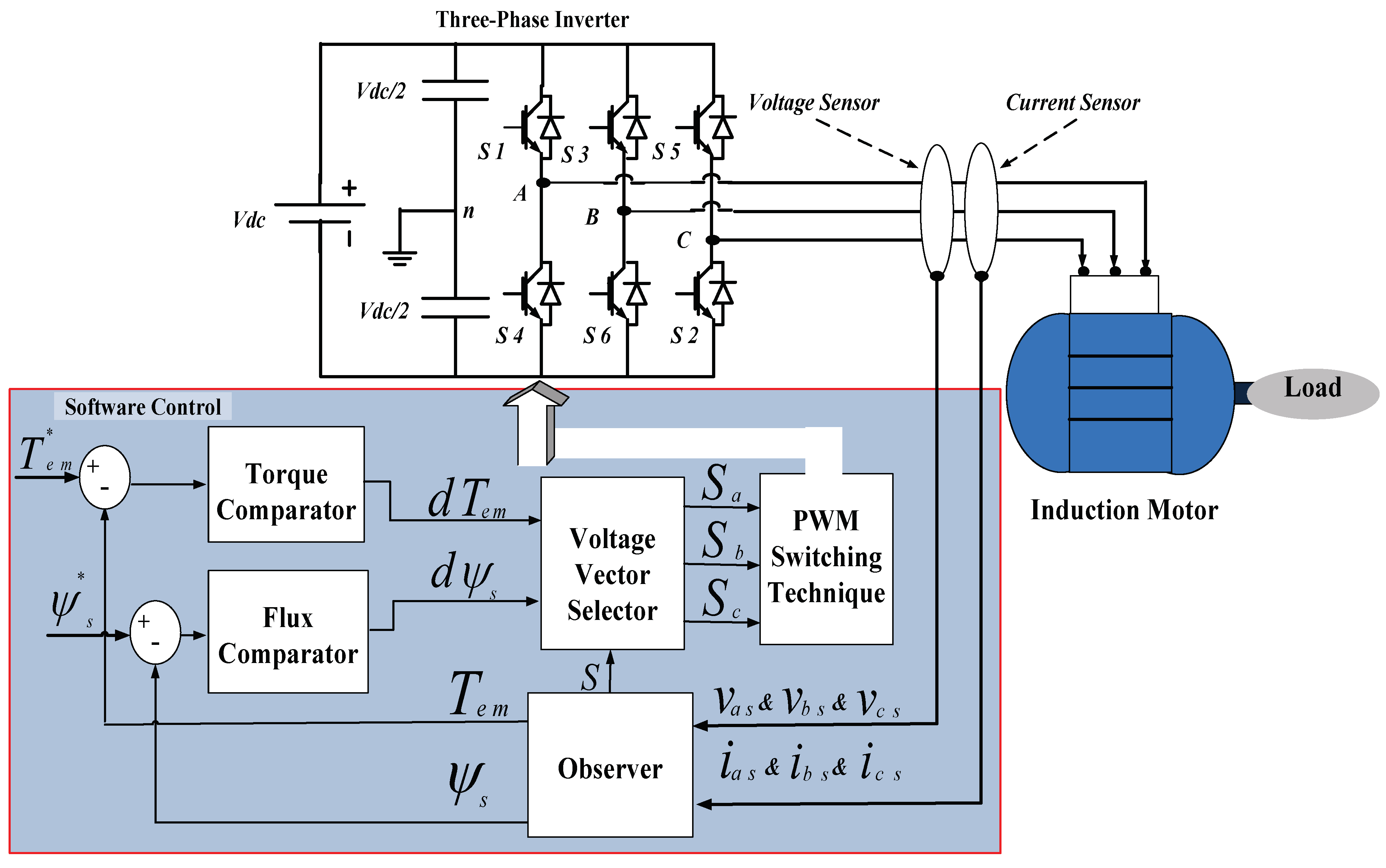
2.2.4. Direct Torque Control

Takahashi suggested another control system recognized as DTC in 1986 [74]. This control method theory is based on the magnitudes of the torque reference and stator flux reference, subtracted from the correspondent calculated feedback signal values. The result is error signals, and these errors are interpreted by controllers of the hysteresis band. To calculate the flux vector number, the feedback signals of the torque and flux are determined from the motor terminal voltages and currents. Through comparators, the torque and flux error produces torque and flux changes. The voltage vector selector is thus subjected to changes in the torque and flux with the flux vector sector number to produce a duty ratio and supply it to the IM, as shown in Figure 11. DTC has numerous benefits over FOC, such as its high dynamic torque response, its simple implementation, less reliance on motor parameters, and no need for a speed sensor [22,25,74]. Nevertheless, DTC has many drawbacks as it requires measuring the current, voltage, and stator resistance. Moreover, DTC presents high noise, variable-switching-frequency behavior, current ripple, and problematic control, particularly under low-speed states [23,33,51,58,59]. Numerous researchers used DTC to enhance various control system applications [32,33,51,58,59,65]. The torque ripples in DTC of an IM drive were reduced via constant switching frequency in [75,76]. A comparison between DTC and FOC to illustrate their advantages and drawbacks was made in [77]. To enhance IM control, VFD through DTC was utilized in [78,79]. DTC was suggested in [75,80] to feed the IM drive through a three-level inverter to reduce the current ripple. The stator flux could be formed as
Ψ α s = (   v α s   i α s   R s   )   dt + Ψ α s ( 0 )
Ψ β s = (   v β s   i β s   R s   )   dt + Ψ β s ( 0 )
where   Ψ α s ( 0 ) and Ψ β s are the stator flux linkages’ initial values. Consequently, the flux magnitude substantially relies on the stator voltage. When the stator voltage changes, the stator flux follows rapidly.
From the stator flux components, the position angle of the stator flux could be calculated as
θ s = tan 1 (   Ψ β s Ψ α s   )
Using the both components of stator current and flux, the electromagnetic torque can be evaluated as
T e = 3 2     P   (   I qs   Ψ ds   I ds   Ψ qs   )
With the exception of stator resistance, the stator flux and electromagnetic torque calculations are independent of the machine parameters.
In summary, the voltage space vectors will regulate the torque. Two voltage vectors are selected in each sector to boost or decrease the stator flux amplitude, as drawn in Figure 12. Based on Figure 12 and Table 2 and Table 3, if the stator flux space vector is presumed to be in sector 1 , V 2 , considering dT em = 1 and d Ψ s = 1 , and V 3 , considering dT em = 1 and d Ψ s = 0 , voltage vectors are applied to increase or decrease the stator flux amplitude, respectively. By applying V 2 or   V 3 , an increase in torque is obtained ( dT em = 1 ). Contrariwise, by applying V 5 or   V 6 , the torque decreases by choosing the suitable voltage vector such that the stator flux amplitude can be held inside a hysteresis band ( dT em = 0 ). If the assessed torque is less than the command value, the voltage vectors that retain the stator flux rotating in the same direction are carefully chosen ( dT em = 1 ) . The load angle will rise, and it will also increase the assessed torque. The zero voltage vectors are selected when the estimated torque exceeds the command one. The load angle falls and thus decreases the electromagnetic torque. The stator flux thus rotates continually, and the orientation is specified by the torque hysteresis controller output. Contrasts of the DTC IM drive, among the scalar and vector control outputs, are displayed in Table 4.
The three-digit numbers in Table 2 describe the switching algorithm where the left-to-right digits give values of   S a   ,   S b , and   S c , respectively. It shows the switching states for regulating the amplitude and orientation of the stator flux.
Values of V α s and V β s in all sectors are displayed in Table 3, where V d equals   2 3     V dc .
A case study has been tested that varies the reference speed from 100 rpm to 500 rpm as shown in Figure 13. The flux and torque are constant with some ripples at rated values. In the motor torque, a chattering phenomenon is introduced. As presented in the literature, one can conclude that the DTC IM drive system is robust with a stator resistance variation. Nevertheless, the energy dissipation variant of the stator resistance may influence the overall performance at the low-speed ranges, so the estimation of the stator resistance may aid to enhancing the drive performance.
A comparison between the performances of the SCC and VC for IMs is presented in Table 4.

3. Control Techniques

3.1. Microprocessor/Digital Control

Control circuitry has been conventionally constructed in the past few decades, beginning with logic hardware and discrete modules with minimal processing power limitations. Improvements in microcontrollers, microcomputers, and microprocessors have had huge consequences for IM drives. They have allowed complex control and sophisticated techniques to be implemented. Traditional control methods were replaced by modern dynamic microprocessor-based control techniques [81,82]. Microprocessor technology development has pursued a fast pace since the first 4-bit microprocessor advent in 1971. Microprocessors evolved from basic 4-bit architectures with minimal functionality to sophisticated 64-bit architectures with enormous processing power in 1992. The control-oriented devices containing a microprocessor and sundry circumferential devices within the same chip are microcontrollers. The microcontroller growth has followed that of the microprocessor and contains three major families: MCS-52, MCS-96, and i960. These families are based on the microprocessor architecture of 8-bit CISC, 16-bit CISC, and 32-bit and 64-bit RISCE, respectively. Digital technologies have progressed in an arrangement as follows: overall purpose microprocessors, microcontrollers, advanced processors (DSPs, RISC, and parallel processors), ASICs, and SoC.
Different efforts have been made in the industrial drives with microprocessor-based control that used modern control theories. Through the Motorola 6800 microprocessor for IMs, a microprocessor-based flux control and slip frequency scheme was presented, and the outcomes were supported by an investigational setup in [83].
A recently built 32-bit microprocessor-based completely numeral control structure was presented to control nonlinear energetic IMs due to rapid changes in microprocessor technology. The high-efficiency microprocessor-based vector-controlled IM drive was described in [84,85], and controller rendering was experimentally tested and confirmed.
The utilization of the billion transistor capacities of a single VLSI-IC has moved the microprocessor routine at an ever-lower cost to an unprecedented stage. DSPs started to emerge around 1979, and currently, advanced parallel processors, DSPs, and RISC processors supply the most demanding implementations with ever-higher computing capabilities. High-execution DSPs could be utilized efficaciously to realize process control techniques with the considerable advances in VLSI and microelectronics technology. Figure 14 illustrates the digital control organization’s basic functions for electric drives.
Embedded systems are computers that are built into devices to perform particular functions for the application. ASIC is a common term utilized to designate any integrated circuit that is specifically built and designed for a specific application. Embedded systems could hold a variety of computing devices, such as microcontrollers, DSPs, and ASICs [86]. Unlike computers, the electronics used in these applications are profoundly embedded and must communicate via sensors and actuators through the operator and the actual word. A key demand is that the computing procedures react continuously in real time to exterior events [87].
The FPGAs are a private category of ASICs that differ from mask-programmed gate-arrays in that end users do their programming at their location without IC masking steps. An FPGA is made of a logic block array that could be linked programmatically to construct various designs. Logical blocks based on one of the following are utilized by present commercial FPGAs: transistor pairs, multiplexers, simple small gates (two NANDs and exclusive ORs), wide fanning AND-OR structures, and look-up tables (LUTs) [88]. Electrically programmable switches, which are executed through one of three key technologies, are utilized to program FPGAs: SRAM, a floating gate, and antifuse. The primary benefit of FPGAs over mask-programmed ASICs is the rapid turnaround that could dramatically minimize the design risk because the FPGA reprogramming can easily and inexpensively correct any design error. Embedded systems have progressed toward high-level multichip module explanations and SoC over the last twenty years.

3.2. Observers

A dynamic structure whose state variables are guesstimates of some other structure (electrical machine) is framed as an observer. Both flux and rotor velocity signals must be assessed to build a speed-senseless/high-performance IM drive structure. Fundamentally, observers are in two categories: open loop and closed loop (divergence among the dual beings, whether or not the observer response is controlled by a corrective term incorporating the observer error). The open-loop observer precision is highly dependent on machine parameters. Robustness against signal noise and parameter mismatches is specified to the closed-loop observer. Different closed-loop observer forms are as follows:
i.
MRAS observer.
ii.
Luenberger observer.
iii.
Sliding mode observer.
iv.
Kalman observer.
The observers can operate not only in the idyllic condition of having a complete assumed model assembly but also in the existence of certain grades of model uncertainty. Observer strategies based on a linearized model do not execute sufficiently and have a restricted choice of action in the presence of nonlinearity operations such as saturation and Coulomb friction that could not be linearized. Therefore, observers are designated for the state estimation of unknown nonlinear systems remnants in a dynamic field of research.

3.2.1. Model Reference Adaptive System Observer

For unstable plants, the linear control laws’ design, whose parameters alter their values through time in a recognized range, is a troublesome and nub problem that implies the necessity for the control algorithm implementation. The control objective is to attain the required framework active behavior despite the lack of information on the accurate plant parameter values. The artistic requests are set out in the MRAS via the reference model corresponding dynamic. Thus, the basic assignment is to design such a control that ensures the minimum error among plant outputs and the reference model; Landau introduced this principle comprehensively in 1979 [89]. Figure 15 demonstrates the MRAS’s basic structure.
The reference model is selected to create a desirable trajectory ω rm   that the plant output ω ^ r must track. The plant controller’s feedback and feed-forward gains are iterated via an adaptation algorithm to minimize the error to zero dynamically.

3.2.2. Luenberger Observer

The working theory of those schemes is based on the point that one observer assesses the rotor flux, and the speed is derived via the error of the stator current and the estimated rotor flux. With an Extended-Luenberger observer (ELO) [90], an adaptive linear observer could be utilized to assess the state vector, where four electric equations of IMs form a linear structure with a changeable parameter (rotor velocity). The following state variable equations describe the motor and observer:
  • Motor:
x ˙ = Ax + Bu ,                       y = Cx
  • Observer:
x ^ ˙ = A ˜ x ^ + Bu + H   ( y ^ y   ) ,                 y ^ = C x ^
The IM electrical equations are described through   A , B , and   C , where the stator current is model output y , while ( H ) is an observer gain matrix. The state vector ( x ) has orthogonal components of stator current and rotor flux in the stationary reference frame (   i ds   , i qs   , Ψ dr , and   Ψ qr ). Matrix A is subject to rotor velocity. If the observer calculates and utilizes the rotor speed, its matrix will be denoted as A ˜ instead of   A , owing to the difference between the actual and estimated speed. The observer gains matrix   H is studied to have observer poles relative to IM poles. The rotor speed is estimated as
ω ^ r = K P   (   Δ ids Ψ ^ qr   Δ iqs Ψ ^ dr ) + K I   0 T (   Δ ids Ψ ^ qr   Δ iqs Ψ ^ dr ) dt
where   Δ ids = (   i ds i ^ ds   ) and   Δ iqs = (   i qs i ^ qs   ) are current errors obtained from the difference between measured and assessed currents, while ( K P , K I )   are adaptation mechanism gains. ELO is appropriate to a nonlinear-time-varying deterministic system.

3.2.3. Sliding Mode Observer

Traditionally, a high-velocity switching regulator action has been applied to switch between various structures, and system state trajectory is obliged to transfer over a selected manifold in state space, named the switching manifold. The sliding surface thus defines the closed-loop system behavior. To achieve a desirable response, the SMC definition is established on varying the controller’s structure based on the system’s changed state [91].
SMC is a main principle of variable structure control (VSC), which is a discontinuous regulator strategy compatible with uncertain nonlinear dynamic schemes. SMC is quick and robust; however, quantity control usually shows undesirable chatter. For inverter-fed drives, the well-known DTC stands as a particular case of VSC wherein consecutive inverter states are chosen based on flux and torque regulator errors. Since VSI is a switching device by its design, it is natural to view the drive regulator from a VSC perspective.
Owing to its high robustness, low computational requirements, and ease of implementation [32,51,58,92,93], it could be carefully chosen. To this end, various SMO structures have been suggested for flux and speed assessment over the last decade.

3.2.4. Kalman Observer

This observer is a mathematical equations set, a method that reduces the mean squared error and provides an effective computational (recursive) means to estimate a process state. In many aspects, the observer is quite powerful: it supports past estimations, and present and even futurity states, and it could do so even if the modeled system’s precise nature is unknown [94]. The three subsequent equations contain the Kalman observer, all involving matrix manipulation.
The subsequent equations contain the following:
The superscript T indicates matrix transposition; the superscript 1 specifies matrix inversion, and the superscript ^ specifies the approximate component. Matrix K is named the Kalman gain, and matrix P is the approximation error covariance.
K k = A   P k   C T   ( C   P k   C T +   S z   ) 1
x ^ k + 1 = (   A   X ^ k + B   u k   ) +   K k   (   y k + 1   C   X ^ k   )
P k + 1 =   A   P k   A T +   S w   A   P k   C T   S z   1   C   P k   A T
where A , B , and C are matrices; x is the system state; k is time index; y is the measured output; and   z and w are the noise. The noise covariance matrices S w and S Z   are defined as follows:
The measurement noise covariance is
S z = E   (   z k   z k T   )
The process noise covariance is
S w = E   (   w k   w k T   )
where z T and w T imply that the random noise vectors w and z are transposed, and E   (   )   is the expectant value.
The fundamental KF is at most viable to the linear stochastic scheme, and the extended Kalman filter (EKF) is utilized for the nonlinear system that stands based on the statistics information of both the state and noise produced via measurement and scheme modeling [24,64,95,96].

3.3. Model Reference Adaptive System Based Control for IMs

With various types of observers, the MRAS is used as an estimator technique. Schemes based on the MRAS method can obtain high-performance dynamic control of sensorless IM drives. The MRAS has been utilized to assess the rotor circuit parameters via Lyapunov’s, Popov’s, fuzzy, and neural techniques for DFOC and IFOC of an IM. The VC drive performance is subject to model parameter deviation; thus, MRAS-based observers via diverse procedures are offered herein. For vector-controlled IMs, efforts have been made to assess the rotor velocity and stator resistance through Popov’s and Lyapunov’s criterion-based AFOO [65,97,98,99]. Stability influences the closed-loop behavior, and MRAS estimator effects contribute to an incorrect estimate. The stability issue induces fluctuation in the drive mechanism, resulting in unstable operation. Oscillations depend more on closed-loop natural momentum than the adaptive MRAS loop’s natural frequency. A sensorless IFOC for IM drives based on the MRAS as an estimator technique is suggested in Figure 16.
To progress drive performance and resolve parameter assessment trouble at low-velocity operation, numerous MRAS closed-loop flux estimators were industrialized in [100,101,102].
A comparative analysis of the adaptive velocity estimator and inherently sensorless velocity observer is obtainable from [103], demonstrating the velocity estimator’s impact on flux observer precision. Theoretical observer review has been performed in addition to experimental testing in this comparative research. This presents the major features of the schemes. Comparative research expanded to embrace three methods of flux and speed observation, i.e.,
  • Torque current components—MRAS;
  • Rotor flux—MRAS;
  • Adaptive nonlinear flux observer.
Based on stability, these three methods have been experimentally analyzed, including also load inertia and bandwidth estimate as described in [104].

3.4. Intelligent Control

It all started with the launch of Minsky and Papert’s book called Perceptrons in 1969 [105] for the artificial neural networks (ANNs) field. Authors have shown, among other examples, that the simple function Exclusive OR could not even be represented via a single-layer perceptron. In the 1980s, when these multilayer ANN training algorithms were proposed, this passive phase was overcome by multilayer ANNs [106]. After that, ANN growth has traversed numerous stages. Cybenko reached the most significant step in 1989. The author has evidenced that ANNs could be utilized as a global approximate [107]. Thereafter, numerous works have been conducted in sundry fields regarding the ANN and its implementation. There have been several of these works in the modeling field. ANNs hold great promise for reproducing linear or nonlinear models and being fault tolerant of the connection or neuron loss. ANNs demonstrated a considerable capability to reproduce controllers in the field of control. Likewise, in the end of the 1960s, the fuzzy logic (FL) field began [41]. Human decision-making simulations are devoted to a large proportion of research/studies in the FL area. For the process control field, the first application appears in [108]. Today, one of the approaches most often used is the fuzzy system. It is feasible to utilize optimization techniques based on the FL speed controller to improve IM drive scalar control, as drawn in Figure 17. The suggested optimization techniques obtain rotor velocity error e and assess objective functions. Such optimization technique targets the achievement of high performance via diminishing objective functions at sudden changes in velocity and mechanical load settings. The optimization technique then looks for minimal error, error adjustment, and membership function (MF) boundaries for both input/output of fuzzy velocity controller to enhancing SCC for IM drives.
To promote the DFOC scheme for IM drives, as manifested in Figure 18, optimization techniques based on FL velocity/flux/torque controllers can be suggested. Figure 18 demonstrates the optimization technique to enhance the adaptive IFOC method for IM drives based on fuzzy dq current controls and fuzzy speed. In both schemes, the optimization technique computes objective functions and receives an error e of the rotor speed. The optimization technique looks for the minimal error, error adjustment, and MF boundaries for the input/output of the FL (velocity/flux/torque) controller for the DFOC structure and fuzzy dq current controllers and fuzzy velocity for IFOC structure after diminishing objective functions at the sudden change in velocity and mechanical load conditions.
Authors have logically tried to merge the FL and ANN in various ways since the early 1990s with a wide range of approaches [109,110,111,112,113,114,115]. The Neuro-Fuzzy Structures (NFS) originated from there. The NFS was classified in [110] with three behaviors: concurrent, fused, and cooperative. The fused NFS are utilized to impart some stationary structures’ internal parameters. Thus, they are deemed to be the most prevalent construction [111]. Jang introduced ANFIS in [112,115], which belongs to fused NFS. ANFIS is called the universal approximation owing to its ability to process any linear or nonlinear function [113]. Figure 19 demonstrates the most popular combination (mixing) among the FL and ANN for the IFOC method.

4. Motor Parameter Estimation

The parameter computation is the major problem that occurs in IM drives. The motor parameters could be easily ascertained through the blocked rotor test and DC test. However, during operation, frequency changes, temperature increases, and load disturbances affect the motor’s parameters. Resistances alter with temperature, whereas inductances vary with the saturation of magnetic material.
Since vector control techniques are very sensitive to motor parameter variance, an essential requirement for obtaining high control performance is to coincide the actual IM parameters with the motor parameters in the FOC. If the error is not modified to the vector controller, machine performance can deteriorate in the form of a steady-state error and transient oscillations in torque, as well as in speed [30,54,97]. In vector control, torque-generating current and flux-producing current are decoupled. However, torque per ampere current remains maximum during both transient and steady-state operation. The flux-/torque-generating current components are correctly calculated from the magnitude of the stator current; however, motor slip s is used for this reason. The rotor time constant τ r is determined from the values of L r   and   R r , thereafter slip determination. Accordingly, for excellent IM drive performance throughout both transient and steady-state conditions, the motor parameters applied in the vector controller must be precise.
Incorrect parameter values in the vector controller also result in the controller de-tuning owing to a mismatch in FOC [116]. The other effects of de-tuning could be summarized as follows: (i) higher stator current magnitude being drawn for the same loading conditions, (ii) improper flux level, (iii) variance in steady-state torque value compared with the reference value, and (iv) non-instantaneous torque responses. Real-time estimating of motor parameters and online updating in the controller may significantly resolve this serious issue [116,117,118,119].
In [97], a sensorless system of vector-controlled IM drives via AFOO, taking core loss into account, was proposed, in which the AFOO was intended for the coinciding assessment of rotor velocity and stator and rotor resistances. Furthermore, a high dynamic performance with a good assessment of the rotor speed and motor parameters was obtained.
The MRAS-based estimate method was suggested and verified experimentally for the rotor resistance variant owing to temperature rise in [120]. ANN and FLC methods for parameter identification were suggested in [116,121].

5. Low-Speed and Field-Weakening Operation

5.1. Low-Speed Operation

The control procedure in the low-speed area is a sophisticated problem in speed-sensorless drives. The stator voltage measurement’s decreased precision in low-speed operation is the primary contributor to this problem. Voltage and current discrepancies and imbalances also contribute to this issue. Many other planned works have made an effort to diminish this problem.
In [122], a robust speed-sensorless technique is designated for guessing the IM speed via measured quantities of voltages and currents. The reactive power instantaneous measurement is the basis of this approach. This technique is not based on the stator resistance value conception, nor is it affected by temperature variation. Moreover, sensed variable integration is not demanded to decrease the computational burden absolutely. Therefore, this method can grasp much wider bandwidth speed control than earlier tacholess drives.
In [123], the authors suggested a new approach to guesstimate the IM speed through stator flux integration. A pure integrator is used for stator flux assessment that allows high-assessment bandwidth. With the use of a self-adjusting inverter model, the system nonlinear voltage distortions are corrected. The strategy has demonstrated high dynamic performance and smooth steady-state operation at extremely low speed. However, it is impossible to estimate the velocity at the zero stator frequency, and further improvements are sought nearer to this area.
It is appropriate to use observers to estimate different plant parameters. The IM velocity and position assessment can be performed via the state-space model [65,92,97,124,125].
A new sensorless Kalman filter technique to estimate the IM velocity that used UKF and SRUKF is suggested in [126]. The SRUKF approach also diminishes the computational issue related to EKF.
In [127], the H_infinity ( H ) theory for the IM velocity estimate is proposed. The advantage of this work is the velocity assessment is used as a control signal in a sensorless FOC drive, and then a motor-wide range speed is developed.
In [34], a speed observer via ANN scheme is suggested. Through the use of the ANN technique for velocity assessment, the drive becomes more robust. It can also be supposed that the controller does not need exact system knowledge and is, therefore, independent of any IM parameter deviations.

5.2. Field-Weakening Operation

The aim is to achieve extreme torque and to completely leverage the machine and converter abilities when IMs are utilized in high-speed applications. Each control system could handle this issue in many ways, varying in terms of performance, complexity, and regulator number and type. The control issue is unclear since the constraints resultant from the stator current and the limited dc-link voltage make it a nonlinear problem [34,90,94,128]. At high speed, the back electromotive force (emf) averts stator currents from circulating in the IM, and thus, the torque decreases. Minimizing the flux level to reach higher speed values is important, but the optimum flux depends on motor velocity, machine parameters, and the dc-link voltage.
Sundry works have attempted to find answers to this issue via suggesting explicit equations of the optimal flux value or calculating LUTs [128,129,130,131]. Nevertheless, these algorithms’ performance is severely linked to the precision by which the parameters are identified, particularly as some parameters may change depending on the frequency, temperature, and also magnetic saturation. As a result, new approaches have been investigated to compensate for the parameter variations and the uncertainties of the models in [131,132,133,134].
Another technique for robust field weakening is to decide the optimal flux level through closed-loop structures that evaluate the IM behavior instead of LUTs or obvious expressions comprising IM parameters [135]. In this work, the flux level is modified based on the supply voltage required by the controllers, and the max torque capacity is subjugated via a convenient control approach.

6. Magnetic Saturation and Core Loss Impact

The iron core losses of electrical IMs working on the sinusoidal power supply are one of the prime losses in electrical machines at 15 25 %   of the overall motor losses [136]. The precise guess of the core loss and motor efficiency demands the precise quantification of the core loss during the motor design procedure, basically for electrical machines’ thermal and electromagnetic design. Stator and rotor core iron losses are owing to space fundamental and harmonic fluxes. These losses comprise eddy current loss, hysteresis loss, and excess losses. The eddy current and hysteresis losses are relative to the supply frequency-square f s 2 and supply frequency   f s , respectively. Inside the machine, the time-varying rotating magnetic flux causes the magnetic material to undergo a cyclical variation, subsequent in hysteresis loss that depends on the frequency and area of the loop. The rotor current frequency is very small under normal motor operation, and therefore, the rotor core hysteresis loss could be ignored, whereas the stator current frequency is similar to that of the supply, so the stator core hysteresis loss is evident.
Another element of the core loss is the eddy current loss. Owing to the emfs induced in the laminations, eddy currents flow in iron core laminations when they are exposed to alternating fluxes. Because of the magnetic skin effect, the eddy currents’ direction in iron core is to oppose the variation in the flux and oblige the magnetic field to the outer surfaces. This phenomenon induces heat in iron cores and eddy current loss.
The remaining part of the core loss, referred to as “excess loss,” is comparative to the 3/2 frequency power and magnetic flux density of iron cores. Excess loss is owing to the non-uniform distribution of magnetic flux density in the laminations, which is caused by both the skin effect and nonlinear diffusions of magnetic flux density. The classical eddy losses are determined on the basis of the assumption that the field distribution is uniform, which is only true for materials operating at large skin depths. As the frequency increases, the skin depth decreases, and excess loss inhabits a lower part of the overall loss at high frequencies when the skin depth is minor [137,138].
The principles of vector control have been conventionally derived on the supposition that the saturation effect may be neglected. Nevertheless, during machine transients, there are no guarantees that the flux magnitude remains in the linear magnetic field. Furthermore, it is desirable to operate IMs at magnetic saturation in numerous variable torque applications to obtain higher torque [21,139,140,141]. In these applications, the modeling approach success depends on the accuracy with which the equivalent-circuit inductances could be calculated. Inductances could vary widely depending on the flux state in various parts of the IMs. In this regard, magnetic saturation remains one of the prime factors affecting the winding inductances that are extremely hard to model analytically. Moreover, the saturation levels inside the machine change with time during transient operation; fluxes are determined through machine currents.
The magnetic circuit saturation of IMs affects the magnetic permeability of iron parts (reduction), the duration of the starting period, the starting current magnitude, the motor thermal capacity, the pulsating torque, the winding insulation, and the starting current on the power system [139,142].
Many applications require a wide range of speeds, with a maximum speed required that greatly exceeds the IM’s rated speed, as is the case for gearless traction drives and high-performance spindle drives [143,144]. In the field-weakening region, the rotor flux reference must be decreased below its esteemed value. The variance of the rotor flux reference implies a variable degree of magnetic flux saturation in the motor, and thus, the magnetizing inductance of the machine is a variable parameter [21,142,143]. So, on the basis of the requisite accuracy of the abovementioned factors, a mathematical model for a saturated motor is justifiable. Therefore, a set of nonlinear time-varying differential equations is required to study the saturated motor transient behavior. The issue of modeling IMs with a saturating magnetic circuit has constantly been a substantial subject.

7. Conclusions

IM drives majorly contribute to industrial power applications or energy transformation from electrical to mechanical or vice versa. A substantial quantity of energy savings can be attained if VFDs are applied to substitute present non-adjustable IM speed drives. In addition, a suitable IM control can reduce losses and improve the drive system performance. This study reviewed various vector control techniques and optimization algorithms used for IM drives. This study has extensively addressed the fundamental concepts and latest developments in these control structures. Most recently, drives have been powered via digital signal processing (DSP) processors. Therefore, this study discusses electric drive control technology trends related to microprocessors/microcomputers.
The FOC-IM drive efficiency depends on a precise speed/flux/torque estimate. Numerous techniques have been used to estimate these quantities in high-performance IMs. Modern control methods (such as FL and ANNs) that provide promising opportunities for future studies have been described as they are currently an alternative approach to traditional control techniques.
A comprehensive review of the literature available on this subject was conducted to provide thorough insight into low-speed and field-weakening operations. In view of the significant impact on the vector-controlled IM drives of motor parameter uncertainties, magnetic saturation, and core loss influence, a detailed discussion has been presented. These proposals are noteworthy contributions to the sophistication of technologies for IM drive controllers. Therefore, the further evolution of optimized controllers for IM drives will govern the market in the future. One of the future trends is to propose additional control-scheme-based artificial intelligence systems that facilitate drive initialization and optimization. Moreover, there is a need for more diagnostic tools that are integrated into the drive. More drives may be connected to the internet, which will enhance monitoring and predictive maintenance with the aid of AI and optimization methods. New applications that directly affect the quality of life (home automation, mechatronics, automotive, alternative energy, power quality, and medical) will require plug-and-play.

Author Contributions

Conceptualization, A.G.M.A.A. and A.A.Z.D.; methodology, A.G.M.A.A. and A.A.Z.D.; software, A.G.M.A.A. and A.A.Z.D.; validation, A.G.M.A.A., A.Y.A., Z.M.A. and A.A.Z.D.; formal analysis, A.G.M.A.A. and A.A.Z.D.; investigation, A.A.Z.D.; resources, A.G.M.A.A. and A.A.Z.D.; data curation, A.G.M.A.A., A.Y.A., Z.M.A. and A.A.Z.D.; writing—original draft preparation, A.G.M.A.A. and A.A.Z.D.; writing—review and editing, A.G.M.A.A., A.Y.A., Z.M.A. and A.A.Z.D.; visualization, A.G.M.A.A. and A.A.Z.D.; supervision, A.A.Z.D. and A.Y.A.; project administration, A.A.Z.D.; funding acquisition, A.A.Z.D. All authors have read and agreed to the published version of the manuscript.

Funding

This research received no external funding.

Data Availability Statement

All data are contained within the article.

Conflicts of Interest

The authors declare no conflict of interest.

References

  1. Wu, B.; Narimani, M. High-Power Converters and AC Drives, 2nd ed.; John Wiley& Sons: New York, NY, USA, 2017; pp. 101–105. [Google Scholar] [CrossRef]
  2. Holtz, J. Sensorless position control of induction motors. In An emerging technology, Proceedings of the AMC’98—Coimbra. 1998 5th International Workshop on Advanced Motion Control, Coimbra, Portugal, 29 June–1 July 1998; IEEE: Piscataway, NJ, USA, 1998; pp. 1–14. [Google Scholar] [CrossRef]
  3. Diab, A.A.Z.; Al-Sayed, A.-H.M.; Mohammed, H.H.A.; Mohammed, Y.S. Literature Review of Induction Motor Drives. In Development of Adaptive Speed Observers for Induction Machine System Stabilization; Springer: Singapore, 2020; pp. 7–18. [Google Scholar] [CrossRef]
  4. Murata, T.; Tsuchiya, T.; Takeda, I. Vector control for induction machine on the application of optimal control theory. IEEE Trans. Ind. Electron. 1990, 37, 283–290. [Google Scholar] [CrossRef]
  5. Koga, K.; Ueda, R.; Sonoda, T. Constitution of V/f control for reducing the steady-state speed error to zero in induction motor drive system. IEEE Trans. Ind. Appl. 1992, 28, 463–471. [Google Scholar] [CrossRef]
  6. Costa, C.A.; Nied, A.; Nogueira, F.G.; Turqueti, M.D.A.; Rossa, A.J.; Dezuo, T.J.M.; Barra, W. Robust Linear Parameter Varying Scalar Control Applied in High Performance Induction Motor Drives. IEEE Trans. Ind. Electron. 2020, 68, 10558–10568. [Google Scholar] [CrossRef]
  7. Otkun, Ö. Newton–Raphson based scalar speed control and optimization of IM. Automatika 2021, 62, 55–64. [Google Scholar] [CrossRef]
  8. Yussif, N.; Sabry, O.H.; Abdel-Khalik, A.S.; Ahmed, S.; Mohamed, A.M. Enhanced Quadratic V/f-Based Induction Motor Control of Solar Water Pumping System. Energies 2020, 14, 104. [Google Scholar] [CrossRef]
  9. Ustun, S.V.; Demirtas, M. Optimal tuning of PI coefficients by using fuzzy-genetic for V/f controlled induction motor. Expert Syst. Appl. 2008, 34, 2714–2720. [Google Scholar] [CrossRef]
  10. Siddavatam, R.P.R.; Loganathan, U. Slip Gain Estimation Scheme for Transient Vector Estimator-Based High-Performance Control of Induction Motor Drives. Trans. Indian Natl. Acad. Eng. 2021, 6, 311–321. [Google Scholar] [CrossRef]
  11. Suetake, M.; da Silva, I.N.; Goedtel, A. Embedded DSP-Based Compact Fuzzy System and Its Application for Induction-Motor $V/f$ Speed Control. IEEE Trans. Ind. Electron. 2010, 58, 750–760. [Google Scholar] [CrossRef]
  12. Almani, M.N.; Hussain, G.A.; Zaher, A.A. An Improved Technique for Energy-Efficient Starting and Operating Control of Single Phase Induction Motors. IEEE Access 2021, 9, 12446–12462. [Google Scholar] [CrossRef]
  13. Ahmad, S.; Mishra, A. Mathematical Modelling, Simulation and Control of Five-Phase Induction Motor Drives. In Proceedings of the International Conference on Emerging Frontiers in Electrical and Electronic Technologies (ICEFEET), Patna, India, 10–11 July 2020; pp. 1–4. [Google Scholar] [CrossRef]
  14. Iftikhar, M.H.; Park, B.-G.; Kim, J.-W. Design and Analysis of a Five-Phase Permanent-Magnet Synchronous Motor for Fault-Tolerant Drive. Energies 2021, 14, 514. [Google Scholar] [CrossRef]
  15. Akroum, H.; Kidouche, M.; Aibeche, A. A dSPACE DSP Control Platform for V/F Controlled Induction Motor Drive and Parameters Identification. In Advances in Computer, Communication, Control and Automation; Springer: Berlin/Heidelberg, Germany, 2011; Volume 121, pp. 305–312. [Google Scholar] [CrossRef]
  16. Munoz-Garcia, A.; Lipo, T.; Novotny, D. A new induction motor V/f control method capable of high-performance regulation at low speeds. IEEE Trans. Ind. Appl. 1998, 34, 813–821. [Google Scholar] [CrossRef] [Green Version]
  17. Dybkowski, M.; Klimkowski, K. Artificial Neural Network Application for Current Sensors Fault Detection in the Vector Controlled Induction Motor Drive. Sensors 2019, 19, 571. [Google Scholar] [CrossRef] [PubMed] [Green Version]
  18. Sathishkumar, H.; Parthasarathy, S. A novel neural network intelligent controller for vector controlled induction motor drive. Energy Procedia 2017, 138, 692–697. [Google Scholar] [CrossRef]
  19. Yin, S.; Xia, J.; Zhao, Z.; Zhao, L.; Liu, W.; Diao, L.; Jatskevich, J. Fast Restarting of Free-Running Induction Motors Under Speed-Sensorless Vector Control. IEEE Trans. Ind. Electron. 2019, 67, 6124–6134. [Google Scholar] [CrossRef]
  20. Srivastava, S.P.; Pathak, M.K. Modified Reference Model for Rotor Flux-Based MRAS Speed Observer Using Neural Network Controller. IETE J. Res. 2018, 65, 80–95. [Google Scholar] [CrossRef]
  21. Perdukova, D.; Palacky, P.; Fedor, P.; Bober, P.; Fedak, V. Dynamic Identification of Rotor Magnetic Flux, Torque and Rotor Resistance of Induction Motor. IEEE Access 2020, 8, 142003–142015. [Google Scholar] [CrossRef]
  22. Reza, C.; Islam, D.; Mekhilef, S. A review of reliable and energy efficient direct torque controlled induction motor drives. Renew. Sustain. Energy Rev. 2014, 37, 919–932. [Google Scholar] [CrossRef]
  23. Maes, J.; Melkebeek, J. Speed-sensorless direct torque control of induction motors using an adaptive flux observer. IEEE Trans. Ind. Appl. 2000, 36, 778–785. [Google Scholar] [CrossRef]
  24. Tabasian, R.; Ghanbari, M.; Esmaeli, A.; Jannati, M. Direct field-oriented control strategy for fault-tolerant control of induction machine drives based on EKF. IET Electr. Power Appl. 2020, 36, 778–785. [Google Scholar] [CrossRef]
  25. Blaschke, F. The principle of field orientation as applied to the new TRANSVECTOR closed loop control system for rotating field machines. Siemens Rev. 1972, 34, 217–220. [Google Scholar]
  26. Hasse, K. Zum dynamischen Verhalten der Asynchron maschine bei Betrieb mit variabler Standerfreqenz und Standerspannung. ETZ-A 1968, 89, 77–81. [Google Scholar]
  27. Farah, N.; Talib, M.H.N.; Shah, N.S.M.; Abdullah, Q.; Ibrahim, Z.; Lazi, J.B.M.; Jidin, A. A Novel Self-Tuning Fuzzy Logic Controller Based Induction Motor Drive System: An Experimental Approach. IEEE Access 2019, 7, 68172–68184. [Google Scholar] [CrossRef]
  28. Hannan, M.A.; Ali, J.A.; Mohamed, A.; Amirulddin, U.A.U.; Tan, N.M.L.; Uddin, M.N. Quantum-Behaved Lightning Search Algorithm to Improve Indirect Field-Oriented Fuzzy-PI Control for IM Drive. IEEE Trans. Ind. Appl. 2018, 54, 3793–3805. [Google Scholar] [CrossRef]
  29. Devanshu, A.; Singh, M.; Kumar, N. An Improved Nonlinear Flux Observer Based Sensorless FOC IM Drive with Adaptive Predictive Current Control. IEEE Trans. Power Electron. 2019, 35, 652–666. [Google Scholar] [CrossRef]
  30. Basic, M.; Vukadinovic, D.; Grgic, I.; Bubalo, M. Speed-Sensorless Vector Control of an Induction Generator Including Stray Load and Iron Losses and Online Parameter Tuning. IEEE Trans. Energy Convers. 2019, 35, 724–732. [Google Scholar] [CrossRef]
  31. Zeb, K.; Ali, Z.; Saleem, K.; Uddin, W.; Javed, M.A.; Christofides, N. Indirect field-oriented control of induction motor drive based on adaptive fuzzy logic controller. Electr. Eng. 2016, 99, 803–815. [Google Scholar] [CrossRef]
  32. Savarapu, S.; Narri, Y. High performance of brain emotional intelligent controller for DTC-SVM based sensorless induction motor drive. J. Supercomput. 2021, 77, 1–22. [Google Scholar] [CrossRef]
  33. Wang, F.; Zhang, Z.; Mei, X.; Rodríguez, J.; Kennel, R. Advanced Control Strategies of Induction Machine: Field Oriented Control, Direct Torque Control and Model Predictive Control. Energies 2018, 11, 120. [Google Scholar] [CrossRef] [Green Version]
  34. Devanshu, A.; Singh, M.; Kumar, N. Nonlinear flux observer-based feedback linearisation control of IM drives with ANN speed and flux controller. Int. J. Electron. 2020, 108, 139–161. [Google Scholar] [CrossRef]
  35. Aktas, M.; Awaili, K.; Ehsani, M.; Arisoy, A. Direct torque control versus indirect field-oriented control of induction motors for electric vehicle applications. Eng. Sci. Technol. Int. J. 2020, 23, 1134–1143. [Google Scholar] [CrossRef]
  36. Hannan, M.A.; Jamal, A.A.; Mohamed, A.; Hussain, A. Optimization techniques to enhance the performance of induction motor drives: A review. Renew. Sustain. Energy Rev. 2018, 81, 1611–1626. [Google Scholar] [CrossRef]
  37. Bennett, S. Nicholas Minorsky and the automatic steering of ships. IEEE Control Syst. Mag. 1984, 4, 10–15. [Google Scholar] [CrossRef]
  38. Borja, P.; Ortega, R.; Scherpen, J.M.A. New Results on Stabilization of Port-Hamiltonian Systems via PID Passivity-Based Control. IEEE Trans. Autom. Control 2020, 66, 625–636. [Google Scholar] [CrossRef]
  39. Ulusoy, S.; Nigdeli, S.M.; Bekdaş, G. Novel metaheuristic-based tuning of PID controllers for seismic structures and verification of robustness. J. Build. Eng. 2020, 33, 101647. [Google Scholar] [CrossRef]
  40. Kim, B.S.; Kim, T.Y.; Park, T.C.; Yeo, Y.K. A model predictive functional control based on proportional-integral-derivative (PID) and proportional-integral-proportional-derivative (PIPD) using extended non-minimal state space: Application to a molten carbonate fuel cell process. Korean J. Chem. Eng. 2018, 35, 1601–1610. [Google Scholar] [CrossRef]
  41. Zadeh, L.A. Fuzzy Sets. In Fuzzy Sets, Fuzzy Logic, and Fuzzy Systems: Selected Papers by Lotfi A. Zadeh; World Scientific: Singapore, 1996; pp. 394–432. [Google Scholar]
  42. Benlaloui, I.; Chrifi-Alaoui, L.; Ouriagli, M.; Khemis, A.; Khamari, D.; Drid, S. Improvement of the induction motor sensorless control based on the type-2 fuzzy logic. Electr. Eng. 2021, 103, 1473–1482. [Google Scholar] [CrossRef]
  43. Lamamra, K.; Batat, F.; Mokhtari, F. A new technique with improved control quality of nonlinear systems using an optimized fuzzy logic controller. Expert Syst. Appl. 2019, 145, 113148. [Google Scholar] [CrossRef]
  44. Xia, Y.; Wang, J.; Meng, B.; Chen, X. Further results on fuzzy sampled-data stabilization of chaotic nonlinear systems. Appl. Math. Comput. 2020, 379, 125225. [Google Scholar] [CrossRef]
  45. De Barros, O., Jr.; Amorim, T.S.; Carletti, D.; Neto, A.F.; Encarnação, L.F. Design of an Enhanced FLC-Based Controller for Selective Harmonic Compensation in Active Power Filters. Electronics 2020, 9, 2052. [Google Scholar] [CrossRef]
  46. Begum, M.; Eskandari, M.; Abuhilaleh, M.; Li, L.; Zhu, J. Fuzzy-Based Distributed Cooperative Secondary Control with Stability Analysis for Microgrids. Electronics 2021, 10, 399. [Google Scholar] [CrossRef]
  47. Chandrasekaran, S.; Durairaj, S.; Padmavathi, S. A Performance Improvement of the Fuzzy Controller-Based Multi-Level Inverter-Fed Three-Phase Induction Motor with Enhanced Time and Speed of Response. J. Electr. Eng. Technol. 2021, 16, 1131–1141. [Google Scholar] [CrossRef]
  48. Bensalem, Y.; Abbassi, R.; Jerbi, H. Fuzzy Logic Based-Active Fault Tolerant Control of Speed Sensor Failure for Five-Phase PMSM. J. Electr. Eng. Technol. 2020, 16, 287–299. [Google Scholar] [CrossRef]
  49. Steczek, M.; Chudzik, P.; Lewandowski, M.; Szelag, A. PSO-Based Optimization of DC-Link Current Harmonics in Traction VSI for an Electric Vehicle. IEEE Trans. Ind. Electron. 2019, 67, 8197–8208. [Google Scholar] [CrossRef]
  50. Acikgoz, H.; Yildiz, C.; Coteli, R.; Dandil, B. DC-link voltage control of three-phase PWM rectifier by using artificial bee colony based type-2 fuzzy neural network. Microprocess. Microsyst. 2020, 78, 103250. [Google Scholar] [CrossRef]
  51. Ganthia, B.P.; Pradhan, R.; Sahu, R.; Pati, A.K. Artificial Ant Colony Optimized Direct Torque Control of Mathematically Modeled Induction Motor Drive Using PI and Sliding Mode Controller. In Recent Advances in Power Electronics and Drives; Kumar, J., Jena, P., Eds.; Springer: Singapore, 2020; pp. 389–408. [Google Scholar] [CrossRef]
  52. Storn, R.; Price, K. Differential evolution—A simple and efficient heuristic for global optimization over continuous spaces. J. Glob. Optim. 1997, 11, 341–359. [Google Scholar] [CrossRef]
  53. Back, T. Evolutionary Algorithms in Theory and Practice: Evolution Strategies, Evolutionary Programming, Genetic Algorithms; Oxford University Press: Oxford, UK, 1996. [Google Scholar]
  54. Duan, F.; Zivanovic, R.; Al-Sarawi, S.; Mba, D. Induction Motor Parameter Estimation Using Sparse Grid Optimization Algorithm. IEEE Trans. Ind. Inform. 2016, 12, 1453–1461. [Google Scholar] [CrossRef]
  55. Sakthivel, V.; Bhuvaneswari, R.; Subramanian, S. Multi-objective parameter estimation of induction motor using particle swarm optimization. Eng. Appl. Artif. Intell. 2010, 23, 302–312. [Google Scholar] [CrossRef]
  56. Ali, J.A.; Hannan, M.A.; Mohamed, A.; Abdolrasol, M.G. Fuzzy logic speed controller optimization approach for induction motor drive using backtracking search algorithm. Measurement 2016, 78, 49–62. [Google Scholar] [CrossRef]
  57. Hu, Z.; Hameyer, K. A Method of Constraint Handling for Speed-Controlled Induction Machines. IEEE Trans. Ind. Electron. 2016, 63, 4061–4072. [Google Scholar] [CrossRef]
  58. Diab, A.A.Z.; Anosov, V.N. Implementation of full order observer for speed sensorless vector control of induction motor drive. In Proceedings of the 2014 15th International Conference of Young Specialists on Micro/Nanotechnologies and Electron Devices (EDM), Novosibirsk, Russia, 30 June–4 July 2014; pp. 347–352. [Google Scholar] [CrossRef]
  59. Boukhalfa, G.; Belkacem, S.; Chikhi, A.; Benaggoune, S. Genetic algorithm and particle swarm optimization tuned fuzzy PID controller on direct torque control of dual star induction motor. J. Central South Univ. 2019, 26, 1886–1896. [Google Scholar] [CrossRef]
  60. Chiang, C.-L.; Su, C.-T. Tracking control of induction motor using fuzzy phase plane controller with improved genetic algorithm. Electr. Power Syst. Res. 2004, 73, 239–247. [Google Scholar] [CrossRef]
  61. Kim, D.H. GA–PSO based vector control of indirect three phase induction motor. Appl. Soft Comput. 2007, 7, 601–611. [Google Scholar] [CrossRef]
  62. Rojas, C.A.; Rodriguez, J.R.; Kouro, S.; Villarroel, F. Multiobjective Fuzzy-Decision-Making Predictive Torque Control for an Induction Motor Drive. IEEE Trans. Power Electron. 2016, 32, 6245–6260. [Google Scholar] [CrossRef]
  63. Mousavi, M.S.; Davari, S.A.; Nekoukar, V.; Garcia, C.; Rodriguez, J. A Robust Torque and Flux Prediction Model by a Modified Disturbance Rejection Method for Finite-Set Model-Predictive Control of Induction Motor. IEEE Trans. Power Electron. 2021, 36, 9322–9333. [Google Scholar] [CrossRef]
  64. Zhao, Q.; Yang, Z.; Sun, X.; Ding, Q. Speed-sensorless control system of a bearingless induction motor based on iterative central difference Kalman filter. Int. J. Electron. 2020, 107, 1524–1542. [Google Scholar] [CrossRef]
  65. Aziz, A.; Rez, H.; Diab, A. Robust Sensorless Model-Predictive Torque Flux Control for High-Performance Induction Motor Drives. Mathematics 2021, 9, 403. [Google Scholar] [CrossRef]
  66. Santiseban, J.; Stephan, R. Vector control methods for induction machines: An overview. IEEE Trans. Educ. 2001, 44, 170–175. [Google Scholar] [CrossRef]
  67. Saidur, R.; Mekhilef, S.; Ali, M.; Safari, A.; Mohammed, H.A. Applications of variable speed drive (VSD) in electrical motors energy savings. Renew. Sustain. Energy Rev. 2012, 16, 543–550. [Google Scholar] [CrossRef]
  68. Gopal, B.T.V.; Shivakumar, E.G.; Ramesh, H.R. Design of Deep Learning Controller for Vector Controlled Induction Motor Drive. In Data Engineering and Communication Technology; Raju, K.S., Senkerik, R., Lanka, S.P., Rajagopal, V., Eds.; Springer: Singapore, 2020; pp. 639–647. [Google Scholar]
  69. Gandhi, K.; Saxena, S.; Ali, M. Vector Control of 3-Phase Induction Motor. MIT Int. J. Electr. Instrum. Eng. 2013, 3, 85–88. [Google Scholar]
  70. Amezquita-Brooks, L.; Liceaga-Castro, J.; Liceaga-Castro, E. Speed and Position Controllers Using Indirect Field-Oriented Control: A Classical Control Approach. IEEE Trans. Ind. Electron. 2013, 61, 1928–1943. [Google Scholar] [CrossRef]
  71. Jemli, M.; Ben Azza, H.; Gossa, M. Real-time implementation of IRFOC for Single-Phase Induction Motor drive using dSpace DS 1104 control board. Simul. Model. Prac. Theory 2009, 17, 1071–1080. [Google Scholar] [CrossRef]
  72. Dominic, D.A.; Chelliah, T.R. Analysis of field-oriented controlled induction motor drives under sensor faults and an overview of sensorless schemes. ISA Trans. 2014, 53, 1680–1694. [Google Scholar] [CrossRef]
  73. Shukla, S.; Singh, B. Reduced Current Sensor Based Solar PV Fed Motion Sensorless Induction Motor Drive for Water Pumping. IEEE Trans. Ind. Inform. 2018, 15, 3973–3986. [Google Scholar] [CrossRef]
  74. Takahashi, I.; Noguchi, T. A New Quick-Response and High-Efficiency Control Strategy of an Induction Motor. IEEE Trans. Ind. Appl. 1986, 22, 820–827. [Google Scholar] [CrossRef]
  75. Yen-Shin, L.; Jian-Ho, C. A new approach to direct torque control of induction motor drives for constant inverter switching frequency and torque ripple reduction. IEEE Trans. Energy Convers. 2001, 16, 220–227. [Google Scholar] [CrossRef]
  76. Sekhar, O.C.; Lakhimsetty, S.; Bhat, A.H. A comparative experimental analysis of fractional order PI controller based direct torque control scheme for induction motor drive. Int. Trans. Electr. Energy Syst. 2020, 31, e12705. [Google Scholar] [CrossRef]
  77. Vasudevan, M.; Arumugam, R.; Paramasivam, S. Real time implementation of viable torque and flux controllers and torque ripple minimization algorithm for induction motor drive. Energy Convers. Manag. 2006, 47, 1359–1371. [Google Scholar] [CrossRef]
  78. Kumar, D.D.; Kumar, N.P. Dynamic torque response improvement of direct torque controlled induction motor. J. Physics Conf. Ser. 2020, 1706, 012100. [Google Scholar] [CrossRef]
  79. Kumar, K.V.P.; Kumar, T.V. Enhanced direct torque control and predictive torque control strategies of an open-End winding induction motor drive to eliminate common-mode voltage and weighting factors. IET Power Electron. 2019, 12, 1986–1997. [Google Scholar] [CrossRef]
  80. Yan, L.; Wang, F. Observer-Predictor-Based Predictive Torque Control of Induction Machine for Robustness Improvement. IEEE Trans. Power Electron. 2021, 36, 9477–9486. [Google Scholar] [CrossRef]
  81. Lin, A.K.; Koepsel, W.W. A Microprocessor Speed Control System. IEEE Trans. Ind. Electron. Control. Instrum. 1977, 24, 241–247. [Google Scholar] [CrossRef]
  82. Gabriel, R.; Leonhard, W.; Nordby, C.J. Field-Oriented Control of a Standard AC Motor Using Microprocessors. IEEE Trans. Ind. Appl. 1980, 16, 186–192. [Google Scholar] [CrossRef]
  83. Sen, P.C.; Trezise, J.C.; Sack, M. Microprocessor Control of an Induction Motor with Flux Regulation. IEEE Trans. Ind. Electron. Control. Instrum. 1981, 28, 17–21. [Google Scholar] [CrossRef]
  84. Koyama, M.; Yano, M.; Kamiyama, I.; Yano, S. Microprocessor-Based Vector Control System for Induction Motor Drives with Rotor Time Constant Identification Function. IEEE Trans. Ind. Appl. 1986, 22, 453–459. [Google Scholar] [CrossRef]
  85. Kadyrov, I.; Karaeva, N.; Andarbekov, Z.; Kadyrkulova, K. Features of Designing a Variable-Frequency Electric Drive Control System with a Microprocessor-Based Sinusoidal Signal Generator. In High-Performance Computing Systems and Technologies in Scientific Research, Automation of Control and Production; Jordan, V., Filimonov, N., Tarasov, I., Faerman, V., Eds.; Springer: Cham, Switzerland, 2020; pp. 201–217. [Google Scholar]
  86. Pham, M.T.; Kim, J.-M.; Kim, C.H. Deep Learning-Based Bearing Fault Diagnosis Method for Embedded Systems. Sensors 2020, 20, 6886. [Google Scholar] [CrossRef]
  87. Heath, S. Embedded Systems Design; Elsevier: Amsterdam, The Netherlands, 2002. [Google Scholar]
  88. Sidek, A.; Som, M.M. A Review of FPGA-based Implementation related to Electrical Engineering and Contribution to MPPT, Converter and Motor Drive Control. Multidiscip. Appl. Res. Innov. 2021, 2, 357–365. [Google Scholar]
  89. Landau, Y.D. Adaptive control: The model reference approach. IEEE Trans. Syst. Man, Cybern. 1984, 14, 169–170. [Google Scholar] [CrossRef]
  90. Zeitz, M. The extended Luenberger observer for nonlinear systems. Syst. Control Lett. 1987, 9, 149–156. [Google Scholar] [CrossRef]
  91. Utkin, V. Variable structure systems with sliding modes. IEEE Trans. Autom. Control 1977, 22, 212–222. [Google Scholar] [CrossRef]
  92. Chen, Y.; Bu, W.; Qiao, Y. Research on the Speed Sliding Mode Observation Method of a Bearingless Induction Motor. Energies 2021, 14, 864. [Google Scholar] [CrossRef]
  93. Krim, S.; Krim, Y.; Mimouni, M.F. Sensorless direct torque control based on nonlinear integral sliding mode controllers for an induction motor drive: Experimental verification. Proc. Inst. Mech. Eng. Part I J. Syst. Control Eng. 2020, 235, 249–268. [Google Scholar] [CrossRef]
  94. Kalman, R.E. A New Approach to Linear Filtering and Prediction Problems. J. Basic Eng. 1960, 82, 35–45. [Google Scholar] [CrossRef] [Green Version]
  95. Madhukar, P.S.; Prasad, L. State Estimation using Extended Kalman Filter and Unscented Kalman Filter. In Proceedings of the International Conference on Emerging Trends in Communication, Control and Computing (ICONC3), Lakshmangarh, India, 21–22 February 2020; pp. 1–4. [Google Scholar] [CrossRef]
  96. Gaikwad, K.A.; Bhanuse, V. State of Charge Estimation Using Extended Kalman Filter. In Advances in Signal and Data Processing; Merchant, S.N., Warhade, K., Adhikari, D., Eds.; Springer: Singapore, 2021; pp. 101–110. [Google Scholar]
  97. Aziz, A.G.M.A.; Diab, A.A.Z.; El Sattar, M.A. Speed Sensorless Vector Controlled Induction Motor Drive Based Stator and Rotor Resistances Estimation Taking Core Losses into Account. In 2017 Nineteenth International Middle East Power Systems Conference (MEPCON); IEEE: Piscataway, NJ, USA; pp. 1059–1068.
  98. Kubota, H.; Matsuse, K.; Nakano, T. DSP-based speed adaptive flux observer of induction motor. IEEE Trans. Ind. Appl. 1993, 29, 344–348. [Google Scholar] [CrossRef]
  99. Ammar, A. Second-order sliding mode-direct torque control and load torque estimation for sensorless model reference adaptive system–based induction machine. Proc. Inst. Mech. Eng. Part I J. Syst. Control Eng. 2020, 235, 15–29. [Google Scholar] [CrossRef]
  100. Wang, Y.; Yang, J.; Li, S.; Yang, G.; Deng, R.; Hussain, H. Multiplane Rotor Resistance Online Estimation Strategy for Multiphase Induction Machine under Non-Sinusoidal Power Supply. IEEE Trans. Power Electron. 2021, 36, 9487–9500. [Google Scholar] [CrossRef]
  101. Misra, P.; Kumar, B. Rotor Resistance Estimation for Improved Performance of MRAS-Based Sensorless Speed Estimation of Induction Motor Drives; Springer: Singapore, 2020; pp. 177–187. [Google Scholar] [CrossRef]
  102. Orlowska-Kowalska, T.; Korzonek, M.; Tarchala, G. Performance Analysis of Speed-Sensorless Induction Motor Drive Using Discrete Current-Error Based MRAS Estimators. Energies 2020, 13, 2595. [Google Scholar] [CrossRef]
  103. Lascu, C.; Boldea, I.; Blaabjerg, F. Comparative study of adaptive and inherently sensorless observers for variable-speed induction-motor drives. IEEE Trans. Ind. Electron. 2006, 53, 57–65. [Google Scholar] [CrossRef]
  104. Ohyama, K.; Asher, G.; Sumner, M. Comparative analysis of experimental performance and stability of sensorless induction motor drives. IEEE Trans. Ind. Electron. 2006, 53, 178–186. [Google Scholar] [CrossRef]
  105. Marvin, M.; Seymour, A.P. Perceptrons; MIT Press: Cambridge, MA, USA, 1969. [Google Scholar]
  106. McClelland, J.L.; Rumelhart, D.E.; PDP Group. Parallel Distributed Processing; MIT Press: Cambridge, MA, USA, 1986. [Google Scholar]
  107. Cybenko, G. Approximation by superpositions of a sigmoidal function. Math. Control Signals, Syst. 1989, 2, 303–314. [Google Scholar] [CrossRef]
  108. Mamdani, E.H.; Assilian, S. An experiment in linguistic synthesis with a fuzzy logic controller. Int. J. Man-Mach. Stud. 1975, 7, 1–13. [Google Scholar] [CrossRef]
  109. Lima, F.; Kaiser, W.; da Silva, I.N.; de Oliveira, A.A.A. Open-loop neuro-fuzzy speed estimator applied to vector and scalar induction motor drives. Appl. Soft Comput. 2014, 21, 469–480. [Google Scholar] [CrossRef]
  110. Jeen-Shing, W.; Lee, C.S.G. Efficient neuro-fuzzy control systems for autonomous underwater vehicle control. In Proceedings of the 2001 ICRA IEEE International Conference on Robotics and Automation, Seoul, Republic of Korea, 21–26 May 2001; Volume 3, pp. 2986–2991. [Google Scholar]
  111. Nauck, D.; Klawonn, F.; Kruse, R. Foundations of Neuro-fuzzy Systems; John Wiley & Sons: Hoboken, NJ, USA, 1997. [Google Scholar]
  112. Jang, J.-S. Neuro-fuzzy Modeling: Architectures, Analyses, and Applications; University of California: Berkeley, CA, USA, 1992. [Google Scholar]
  113. Jang, J.-S.R. ANFIS: Adaptive-Network-Based Fuzzy Inference System. IEEE Trans. Syst. Man Cybern. 1993, 23, 665–685. [Google Scholar] [CrossRef]
  114. Hanumanthakari, S. Comparative Analysis of Different Types of Membership Functions for Fuzzy Logic Controller in Direct Torque Control of Induction Motor. In Intelligent Computing in Control and Communication; Springer: Singapore, 2021; pp. 405–416. [Google Scholar] [CrossRef]
  115. Sada, S.; Ikpeseni, S. Evaluation of ANN and ANFIS modeling ability in the prediction of AISI 1050 steel machining performance. Heliyon 2021, 7, e06136. [Google Scholar] [CrossRef] [PubMed]
  116. Zeb, K.; Uddin, W.; Haider, A.; Belal, S.; Mehmood, C.A.; Khan, M.A.; Kim, H.J. Robust speed regulation of indirect vector control induction motor using fuzzy logic controllers based on optimization algorithms. Electr. Eng. 2017, 100, 787–802. [Google Scholar] [CrossRef]
  117. Yang, S.; Ding, D.; Li, X.; Xie, Z.; Zhang, X.; Chang, L. A Novel Online Parameter Estimation Method for Indirect Field Oriented Induction Motor Drives. IEEE Trans. Energy Convers. 2017, 32, 1562–1573. [Google Scholar] [CrossRef]
  118. Zerdali, E. A Comparative Study on Adaptive EKF Observers for State and Parameter Estimation of Induction Motor. IEEE Trans. Energy Convers. 2020, 35, 1443–1452. [Google Scholar] [CrossRef]
  119. Zhao, H.; Eldeeb, H.H.; Wang, J.; Zhan, Y.; Xu, G.; Mohammed, O.A. Online Estimation of Rotor Temperature in Induction Motors Based on Parameter Identification. In Proceedings of the 2019 IEEE Energy Conversion Congress and Exposition (ECCE), Baltimore, MD, USA, 29 September–3 October 2019; pp. 1629–1634. [Google Scholar] [CrossRef]
  120. Cao, P.; Zhang, X.; Yang, S.; Xie, Z.; Zhang, Y. Reactive-Power-Based MRAS for Online Rotor Time Constant Estimation in Induction Motor Drives. IEEE Trans. Power Electron. 2018, 33, 10835–10845. [Google Scholar] [CrossRef]
  121. Mahsahirun, S.N.; Yusof, Z.M.; Idris, N.R.N. Offline Artificial Neural Network Rotor Flux Estimator for Induction Motor. In Proceedings of the IEEE 2nd International Conference on Artificial Intelligence in Engineering and Technology (IICAIET), Kota Kinabalu, Malaysia, 26–27 September 2020; pp. 1–6. [Google Scholar]
  122. Fang-Zheng, P.; Fukao, T. Robust speed identification for speed-sensorless vector control of induction motors. IEEE Trans. Ind. Appl. 1994, 30, 1234–1240. [Google Scholar] [CrossRef]
  123. Holtz, J.; Juntao, Q. Sensorless vector control of induction motors at very low speed using a nonlinear inverter model and parameter identification. IEEE Trans. Ind. Appl. 2002, 38, 1087–1095. [Google Scholar] [CrossRef]
  124. Talla, J.; Leu, V.Q.; Smidl, V.; Peroutka, Z. Adaptive Speed Control of Induction Motor Drive with Inaccurate Model. IEEE Trans. Ind. Electron. 2018, 65, 8532–8542. [Google Scholar] [CrossRef]
  125. Orlowska-Kowalska, T.; Korzonek, M.; Tarchala, G. Stability Improvement Methods of the Adaptive Full-Order Observer for Sensorless Induction Motor Drive—Comparative Study. IEEE Trans. Ind. Inform. 2019, 15, 6114–6126. [Google Scholar] [CrossRef]
  126. Jafarzadeh, S.; Lascu, C.; Fadali, M.S. Square Root Unscented Kalman Filters for State Estimation of Induction Motor Drives. IEEE Trans. Ind. Appl. 2013, 49, 92–99. [Google Scholar] [CrossRef]
  127. Diab, A.A.Z.; El-Sayed, A.-H.M.; Abbas, H.H.; Sattar, M.A. Robust Speed Controller Design Using H_infinity Theory for High-Performance Sensorless Induction Motor Drives. Energies 2019, 12, 961. [Google Scholar] [CrossRef] [Green Version]
  128. Wang, B.; Zhang, J.; Yu, Y.; Zhang, X.; Xu, D.G. Unified Complex Vector Field-Weakening Control for Induction Motor High-Speed Drives. IEEE Trans. Power Electron. 2020, 36, 7000–7011. [Google Scholar] [CrossRef]
  129. Accetta, A.; Cirrincione, M.; Pucci, M.; Sferlazza, A. State Space-Vector Model of Linear Induction Motors Including End-Effects and Iron Losses Part I: Theoretical Analysis. IEEE Trans. Ind. Appl. 2019, 56, 235–244. [Google Scholar] [CrossRef]
  130. Lin, P.; Lai, Y. Novel Voltage Trajectory Control for Field-Weakening Operation of Induction Motor Drives. IEEE Trans. Ind. Appl. 2011, 47, 122–127. [Google Scholar] [CrossRef]
  131. Zhang, X.; Wang, B.; Yu, Y.; Zhang, J.; Dong, J.; Xu, D.G. Analysis and Optimization of Current Dynamic Control in Induction Motor Field-Weakening Region. IEEE Trans. Power Electron. 2020, 35, 8860–8866. [Google Scholar] [CrossRef]
  132. Zhang, X.; Foo, G.H.B.; Rahman, M.F. A Robust Field-Weakening Approach for Direct Torque and Flux Controlled Reluctance Synchronous Motors with Extended Constant Power Speed Region. IEEE Trans. Ind. Electron. 2019, 67, 1813–1823. [Google Scholar] [CrossRef]
  133. Tarvirdilu-Asl, R.; Nalakath, S.; Xia, Z.; Sun, Y.; Wiseman, J.; Emadi, A. Improved Online Optimization-Based Optimal Tracking Control Method for Induction Motor Drives. IEEE Trans. Power Electron. 2020, 35, 10654–10672. [Google Scholar] [CrossRef]
  134. Accetta, A.; Alonge, F.; Cirrincione, M.; D’Ippolito, F.; Pucci, M.; Rabbeni, R.; Sferlazza, A. Robust Control for High Performance Induction Motor Drives Based on Partial State-Feedback Linearization. IEEE Trans. Ind. Appl. 2019, 55, 490–503. [Google Scholar] [CrossRef]
  135. Casadei, D.; Serra, G.; Tani, A.; Zarri, L. A Robust Method for Field Weakening Operation of Induction Motor Drives with Maximum Torque Capability. In Proceedings of the Conference Record of the 2006 IEEE Industry Applications Conference Forty-First IAS Annual Meeting, Tampa, FL, USA, 8–12 October 2006; Volume 1, pp. 111–117. [Google Scholar] [CrossRef]
  136. Nasir, B.A. An Accurate Iron Core Loss Model in Equivalent Circuit of Induction Machines. J. Energy 2020, 2020, 1–10. [Google Scholar] [CrossRef]
  137. Mthombeni, T.L.; Pillay, P. Physical Basis for the Variation of Lamination Core Loss Coefficients as a Function of Frequency and Flux Density. In Proceedings of the IECON 2006 - 32nd Annual Conference on IEEE Industrial Electronics, Paris, France, 7–10 November 2006; pp. 1381–1387. [Google Scholar] [CrossRef]
  138. Kowal, D.; Sergeant, P.; Dupré, L.; Vandenbossche, L. Comparison of Iron Loss Models for Electrical Machines with Different Frequency Domain and Time Domain Methods for Excess Loss Prediction. IEEE Trans. Magn. 2015, 51, 1–10. [Google Scholar] [CrossRef]
  139. Grotstollen, H.; Wiesing, J. Torque capability and control of a saturated induction motor over a wide range of flux weakening. IEEE Trans. Ind. Electron. 1995, 42, 374–381. [Google Scholar] [CrossRef]
  140. Liu, L.; Du, X.; Shen, S. Indirect field-oriented torque control of induction motor considering magnetic saturation effect: Error analysis. IET Electr. Power Appl. 2017, 11, 1105–1113. [Google Scholar] [CrossRef]
  141. Lipcak, O.; Bauer, J. Offline method for experimental identification of load-dependent saturation of induction motor taking into account variation of inverse rotor time constant. IET Power Electron. 2020, 13, 1828–1836. [Google Scholar] [CrossRef]
  142. Hughes, A.; Drury, B. Electric Motors and Drives: Fundamentals, Types and Applications; Newnes: London, UK, 2019. [Google Scholar]
  143. Levi, E.; Mingyu, W. A speed estimator for high performance sensorless control of induction motors in the field weakening region. IEEE Trans. Power Electron. 2002, 17, 365–378. [Google Scholar] [CrossRef]
  144. Denkena, B.; Bergmann, B.; Klemme, H. Cooling of motor spindles—A review. Int. J. Adv. Manuf. Technol. 2020, 110, 1–22. [Google Scholar] [CrossRef]
Figure 1. IM control system design.
Energies 16 02854 g001
Figure 2. Classification of the VFD methods.
Energies 16 02854 g002
Figure 3. Scalar closed-loop control for IM drive.
Energies 16 02854 g003
Figure 4. Transformation of the rotor flux vector.
Energies 16 02854 g004
Figure 5. (a). Block diagram of DFOC via flux sensor for IM drive. (b). Block diagram of DFOC via rotor flux estimator or observer for IM drive.
Energies 16 02854 g005
Figure 6. Performance of DFOC for IM drive at low-speed operation.
Energies 16 02854 g006
Figure 7. Performance of DFOC IM drive with stator–rotor resistance variations by 50%.
Energies 16 02854 g007
Figure 8. Block diagram of IFOC for IM drive.
Energies 16 02854 g008
Figure 9. Performance of IFOC IM drives at load disturbance and parameter variation in low-speed operation.
Energies 16 02854 g009
Figure 10. Performance of IFOC IM drive under field-weakening operation.
Energies 16 02854 g010
Figure 11. Block diagram of DTC for IM drive.
Energies 16 02854 g011
Figure 12. Stator voltage vectors and sectors.
Energies 16 02854 g012
Figure 13. Performance of DTC IM drive.
Energies 16 02854 g013
Figure 14. Block diagram of digital control techniques.
Energies 16 02854 g014
Figure 15. MRAS scheme.
Energies 16 02854 g015
Figure 16. IFOC block diagram for IM drive based on MRAS.
Energies 16 02854 g016
Figure 17. Optimization technique for scalar control based on FL speed controller.
Energies 16 02854 g017
Figure 18. Optimization technique for DFOC based on FLC.
Energies 16 02854 g018
Figure 19. (a) Optimization technique for IFOC based on mixing ANN and FLC. (b). Optimization technique for IFOC based on FLC.
Energies 16 02854 g019
Table 1. IM parameters.
SymbolParametersValues
v s Rated voltage 380   V
n p No. pole pairs 1
f Rated frequency 50   Hz
R s Stator resistance 1.2   Ω
R r Rotor resistance 1   Ω
L s Stator self-inductance   175 × 10 3   H
L r Rotor self-inductance   175 × 10 3   H
L m Magnetizing inductance   170 × 10 3   H
J Moment of inertia   0.062   Kgm 2
Ψ sn Nominal stator flux 0.71   wb
T n Nominal torque 20   Nm
R m Core resistance 2.186   K Ω
T s Sampling time   4 × 10 5   s .
Table 2. Inverter switching states.
Sector Number ( θ ) d Ψ s = 1 d Ψ s = 0
d T e m = 1 d T e m = 0 d T e m = 1 d T e m = 0
1 V 2
( 110 )
V 6
( 101 )
V 3
( 010 )
V 5
( 001 )
2 V 3
( 010 )
V 1
( 100 )
V 4
( 011 )
V 6
( 101 )
3 V 4
( 011 )
V 2
( 101 )
V 5
( 001 )
V 1
( 100 )
4 V 5
( 001 )
V 3
( 010 )
V 6
( 101 )
V 2
( 110 )
5 V 6
( 101 )
V 4
( 011 )
V 1
( 100 )
V 3
( 010 )
6 V 1
( 100 )
V 5
( 001 )
V 2
( 110 )
V 4
( 011 )
d Ψ s and dT em   are outputs of the flux and torque hysteresis controllers, respectively, and θ is the sector number.
Table 3. Stationary (α-β) stator voltages.
V 1 V 2 V 3 V 4 V 5 V 6 V 7 V 8
V α s V d 1 2   V d 1 2   V d   V d 1 2   V d 1 2   V d 00
V β s 0 3 2   V d 3 2   V d 0 3 2   V d 3 2   V d 00
Table 4. Comparison of SCC and VC performances.
Scalar ControlVector Control
Prototype implementationEasy design-in prototype implementationProblematic design in a prototype implementation
CostLow costHigh cost
StructureSimple structureComplex structure
Parameter dependency Without the requirement for IM parameter identificationNecessitates and is sensible to IM parameters
Low-speed operationPoor performance when operating at low velocitiesHigh rendering in FOC and low performance of DTC in low-velocity responses
Sensors needed Only velocity sensorMany sensors are required:
six sensors in DFOC,
four sensors in IFOC, and
six sensors in DTC
Coordinate transformationsWithout requirement for coordinate transformationsEspecially in FOC, it must be transformed in coordinates
RipplesMinimizes the ripple of currentHigh-current/torque ripple in DTC
Disclaimer/Publisher’s Note: The statements, opinions and data contained in all publications are solely those of the individual author(s) and contributor(s) and not of MDPI and/or the editor(s). MDPI and/or the editor(s) disclaim responsibility for any injury to people or property resulting from any ideas, methods, instructions or products referred to in the content.

