Article

Cumulative Interactions between the Global Blockage and Wake Effects as Observed by an Engineering Model and Large-Eddy Simulations

1
Renewables, UL International GmbH, 26122 Oldenburg, Germany
2
Institute of Flight Guidance, Technical University of Braunschweig, 38106 Braunschweig, Germany
3
ForWind, Institute of Physics, Carl von Ossietzky University Oldenburg, 26129 Oldenburg, Germany
4
UL International, Richmond, BC V6V 2V4, Canada
*
Author to whom correspondence should be addressed.
Energies 2023, 16(7), 2949; https://doi.org/10.3390/en16072949
Submission received: 31 January 2023 / Revised: 7 March 2023 / Accepted: 21 March 2023 / Published: 23 March 2023
(This article belongs to the Section A3: Wind, Wave and Tidal Energy)

Abstract

:
By taking into account the turbine type, terrain, wind climate and layout, the effects of wind turbine wakes and other losses, engineering models enable the rapid estimation of energy yields for prospective and existing wind farms. We extend the capability of engineering models, such as the existing deep-array wake model, to account for additional losses that may arise due to the presence of clusters of wind farms, such as the global blockage effect and large-scale wake effects, which become more significant with increasing thermal stratification. The extended strategies include an enhanced wind-farm-roughness approach which assumes an infinite wind farm, and recent developments account for the upstream flow blockage. To test the plausibility of such models in capturing the additional blockage and wake losses in real wind farm clusters, the extended strategies are compared with large-eddy simulations of the flow through a cluster of three wind farms located in the German sector of the North Sea, as well as real measurements of wind power within these wind farms. Large-eddy simulations and wind farm measurements together suggest that the extensions of the Openwind model help capture the different flow features arising from flow blockage and cluster effects, but further model refinement is needed to account for higher-order effects, such as the effect of the boundary-layer height, which is not currently included in standard engineering models.

1. Introduction

The presence of a wind farm disturbs the atmospheric boundary layer (ABL) flow in a number of ways that must be taken into account when estimating wind farm energy yields. In the region situated immediately upstream of a wind farm, the net thrust of the farm makes it act as a porous obstacle to the flow, resulting in a small but significant deceleration of the flow upstream of the wind farm known as the global blockage effect, and flow acceleration around and above the wind farm; the latter may trigger internal gravity waves above the farm, resulting in additional drag [1]. While blockage can impact all rows of the wind farm, the effect is most pronounced in the first row. Within the wind farm, the individual wind turbine wakes expand downstream and gradually join, which reduces the wind speed quickly behind the first row of wind turbines and more gradually with each successive row due to turbulent diffusion. In the downstream, far-field of a wind farm, the individual wind turbine wakes together with the distortion of the flow, due to the wind farm as a whole, result in large-scale farm-integrated wakes that can extend many tens of kilometres downstream [2,3]. The energy yield from downstream wind farms may consequently be affected by the wake of upstream wind farms [4], which seems to be the case in the North Sea, for instance. The significance of these effects depends, at least, on the wind farm geometry, wind turbine thrust, the degree of stratification, the level and the ambient turbulence, the terrain including the surface roughness, and the ABL height. The challenge is to incorporate some of these effects into engineering models, such as Openwind [5] (a wind farm design and optimization software tool), which are used for the optimization of wind farm layouts and energy yield estimation.
In general terms, wind farm design/optimization and energy yield assessment tools, such as Openwind, take into account the topography, and use environmental features (e.g., visual, noise and shadow flicker), wind turbine technology, and local meteorology to produce an optimized design of a prospective wind farm [5]. As this optimization needs a large number of calculations of different configurations, it is required that the wake model physics modules run as quickly as possible, which means that the flow within and around a wind farm has to be greatly simplified. For large wind farms and in order to account for coupled ABL–wake interactions, the deep-array wake model (DAWM; [6]) within the Openwind software is a well-known approach among fast engineering models. The DAWM approach is based on the surface-drag-induced internal-ABL concept of Frandsen [7] to modify the wind speed profile within the ABL with an increasing distance downstream of the front of a turbine array. For a comparison of different commercial models, please refer to [8]. This may be combined with the wind speed reduction downstream of wind turbines, i.e., wind turbine wakes, which is a standard component of such engineering models (e.g., [9,10,11]), and is the focus of continual research and development [12].
Compared with wind turbine wakes, the wind speed reduction upstream of turbines, i.e., the blockage effect, has received less attention, and has only recently been included in the Openwind calculations using recently described wind turbine induction models [13,14,15]. Wind farm-scale blockage, i.e., global blockage, may also be caused by upstream flow deceleration in response to the generation of gravity waves above and downstream of wind farms [1,16,17,18]. Moreover, in large wind farms, as is the case offshore, gravity waves drive significant pressure gradients in the boundary layer and play an important role in redistributing energy throughout the wind farm [16]. Since the significance of the blockage may amount to approximately 2–5% of the freestream wind speed [19], this is an effect that needs to be assessed and estimated in the wind farm design phase.
To accommodate the rapid growth and demands of the offshore wind energy industry, particularly in the North Sea, far-field wake effects to account for upstream wind farm clusters are also modeled in Openwind.
For example, directly downstream of an offshore wind farm, the wind speed may be reduced to between 50% and 75% of the freestream wind speed, and, depending on the atmospheric stability, may only recover to freestream values some 20–80 km downstream [2]. The DAWM approach may take far-field effects into account but does not consider stability effects at this stage. Hence, the top-down wake model approach suggested by Emeis [20] seems to be a promising alternative because it takes stability into account explicitly and has already been proven to be plausible when compared with far-field wake measurements derived from flight data [2]. Another promising option could be the three-layer model proposed by Allaerts and Meyers [17], which is able to estimate the gravity-wave-induced flow modifications, including induction effects around wind farms, by incorporating ABL information such as wind speed and temperature profiles, the ABL height, and the stratification in the free atmosphere.
As wind farm flows are turbulence-driven processes, turbulence-resolving models are evidently a proper way to gain a better understanding of these flows. Therefore, the best tool for assessing the performance of novel flow models for engineering purposes is the large-eddy simulation (LES), which explicitly resolves the large-scale turbulent motions by integrating the filtered Navier–Stokes equations in time and parameterizes the impact of small-scale turbulence on the resolved scales (subgrid-scale turbulence) using some form of turbulence diffusion. The Parallelized LES Model (PALM) is one such LES model that is used extensively for fundamental ABL research [21,22] and more recently has been adopted for research in wind energy by inclusion of the actuator-disc approach to model the thrust of wind turbines (e.g., [23,24,25,26]).
The high computational demand of LES models, which is due to the large domain and grid resolution required for simulating a large offshore wind farm, limits the number of flow cases that can be investigated, and thus can only be used as a first reference. For example, initial comparisons of PALM results with some of the induction models mentioned above reveal their underestimation of the global blockage in idealized small (3 × 3 and 7 × 7 turbines) wind farms [27]. Stieren and Stevens [28] used another LES model to simulate an idealized wind farm cluster with two wind farms (each with 12 × 6 turbines) separated by 10 km and evaluated the performance of four engineering models, taking the LES results as a reference. It was found by means of a single neutral case that all considered models overestimate the wind farm wake recovery compared to what is observed in the LES results.
Our objective is to evaluate the performance of the existing Openwind DAWM approach and provide detailed flow simulations to aid in the development of the stability-dependent wind farm model based on the proposal of Emeis [20]. For this purpose, we have selected a number of typical ABL conditions for the explicit LES treatment of the flow upstream from, through and downstream of a wind farm cluster in the North Sea for quantification of the scale of the global blockage and wind farm wake recovery in large wind farms. The key parameters varied are the boundary-layer height and stability: neutral conditions are simulated for boundary-layer heights of approximately 300 m, 500 m, and 900 m above sea level, and weakly stable conditions for a boundary-layer height of approximately 300 m. We are interested principally in the resulting wind speed at a hub height produced by the LES model and the corresponding wind power generated, and these are to be compared with the outputs of the Openwind model.
Section 2 introduces the Openwind model and the wake and induction modules used in the flow simulations of the wind farm cluster, which is briefly described in Section 3. The LES set-up and boundary conditions are described in Section 4. The LES wind speeds and the comparison with the Openwind wind speeds are presented in Section 5. Both LES and Openwind wind powers are then compared with the real measured wind power in Section 5.2. These results are brought together and then summarized in a discussion in Section 6 and in the conclusions in Section 7, respectively.

2. Description of the Openwind Engineering Model Suite

Rapid engineering wake models are the most common tools used by the industry for wind farm design and optimization throughout the wind project development process. The aim is to create optimal turbine layouts that maximize energy production, minimize energy losses, account for wind farm development costs and deliver project efficiencies, ultimately yielding an estimate of the wind farm’s power production as accurately as possible. The computational cost of engineering models must be low, since many iterations, encompassing the combination of multiple wind conditions (wind speed and direction), are required to determine an optimized wind farm design. This requires accurate but computationally efficient physics modules within the Openwind model, so that a maximum number of layouts can be considered.
In the widely used wind farm design and optimisation software, “Openwind” [5], some of the basic inputs into the model are wind speeds and directions from one or more meteorological masts at the hub height at the proposed site, details of the terrain and specifications (e.g., power curves) of the proposed wind turbines. Wind turbine thrust curves are also needed to take into account the strengths of the turbine wakes (and turbine induction or blockage), which affect the energy output depending on the wind farm layout. The standard set-up for the estimation of wakes from offshore wind farms is the DAWM eddy viscosity (EV) approach, which accounts for the two-way interactions between large deep-array wake effects and the ABL as well as direct turbine on turbine wakes through the EV model [10]. Please refer to [29] for a description of the turbulence closure. Unlike wake effects, blockage effects, which account for the reduction of the incident wind speed in front of a wind farm, have been ignored by such software tools until a few years ago.

2.1. Wake and Blockage Models

Here, we describe adjustments and additions to the standard Openwind DAWM set-up to account for global blockage. Since the DAWM approach does not account for thermal stratification, the approach of Emeis [20] combined with the TurbOPark model [30] to account for wakes are adapted for Openwind, which includes both wake and blockage effects. Table 1 gives details of the parameters used to simulate neutral and stable conditions for comparison with the LES results below.

2.1.1. Deep Array Wake Model (DAWM)

The DAWM approach assumes that a large wind farm many rows deep acts as an increased source of surface roughness and generates an internal boundary layer of reduced wind speed. Two approaches are used in the DAWM: one is the surface-drag-induced internal-ABL approach based on the top-down model proposed by Frandsen [7], which modifies the wind speed profile with increasing distance downstream of the upstream edge of a turbine array. Whilst being characterized as similar in principle to the Frandsen top-down approach, the actual DAWM implementation is bottom up in the sense that the ABL drag emerges as the combination of many small patches of increased roughness, each one being associated with a turbine in the array. The second approach uses a standard “eddy viscosity” (EV; [10]) wake model, where wake width and the velocity deficit are defined by solving the linearized Reynolds-averaged Navier–Stokes equations for the entire velocity field of the far-wake flow (≈2–3 D behind the rotor). This wake model has a Gaussian cross-section and the recovery of the wake depends on the turbulence intensity. The EV model automatically fulfills the conservation of mass and momentum in the wake. In the standard set-up, which does not account for atmospheric stability, the main DAWM parameters are the wind-farm-equivalent roughness length and the wake width angle, with default values for offshore wind farms of 1.16 m and 7 . 5 , respectively, according to previous validation efforts [6]. To account for blockage, the vortex-cylinder model of Branlard and Gaunaa [13], the self-similar model of Troldborg and Meyer Forsting [14] and the Rankine-half-body (RHB) model of [15] (standard set-up) may be used. A comparison of the different induction models with the LES results is provided in Appendix A. Here, all Openwind simulations are performed with the RHB model because of its seemingly superior performance. For the current Openwind configuration, offshore wind farms are simulated by combining the DAWM approach with the EV wake model and an induction model in the following way:
  • The EV and DAWM models are run for each wind turbine in turn, starting with the most upstream turbine, so that as each turbine’s wake is calculated, the incident wind speed, the minimum of that calculated using the DAWM and EV models for each upwind turbine, is already known and the appropriate value of the thrust coefficient C T can be used.
  • If a blockage model is used, this is run with the values of C T used in the wake model, and the resulting wind speed deficits, blockage and wake, are combined as the linear superposition of both.
  • There is an option to pre-run the blockage model before the wake model in order to modify the C T values used in the wake, but it has been found that this option does not add anything in terms of accuracy and so is not recommended.

2.1.2. Array-Stability Model (ASM)

For non-neutral conditions, the DAWM set-up is replaced by a stability-dependent array-compensation model, mostly based on Emeis [20], but enhanced to take into account non-infinite wind farms with global blockage, and described in Appendix B. Inputs to the model are the background roughness length z 0 , and the wind farm layout and corresponding wind turbine thrust coefficients. From that, the effective wind farm drag coefficient C t , e f f is determined. Rather than this being a single parameter for the entire wind farm as in Emeis [20], C t , e f f is distributed in space using a skewed-Gaussian distribution, with the skew to account for a weaker upstream flow induction compared with the wake strength, as described in Appendix B. The wind speed ratio R U 0 (Equation (A7)) throughout and around the wind farm is then calculated by inserting C t , e f f and the turbine hub height h, specifying the ambient turbulence intensity I u , Monin–Obukhov stability parameter z / L , and the quantity Δ z 1 representing the length scale of the turbulent exchange between the wind farm layer and free atmosphere within the wind farm.
The farm wind speed ratio R U 0 is then used as an input to calculate the wind speed ratio R U (Equation (A3)) in the wake based on the recovery rate α . Inputs to this part of the model require the stability function ϕ m ; the friction velocity u * , which is estimated from the freestream wind speed profile for U ; and the quantity Δ z 2 , representing the scale of turbulent exchange in the wake and the free atmosphere.
The ASM model is implemented in OpenWind in the following way:
  • The wind speed ratio R U 0 ( x , y ) is calculated at each grid point and then R U ( x , y , N ) is found downstream of each grid point N;
  • The absolute minimum of U R ( x , y , : ) is then calculated from which the value of U R at each turbine is used to estimate C T ;
  • The TP (TurbOPark) wake model is run for each turbine using the freestream modified by the ASM;
  • The minimum wind speed for the TP and farm models is taken as the modelled wind speed.

3. Case Study: The N-4 Offshore Wind Farm Cluster

We investigate the flow around the German offshore N-4 cluster located around 80 km north of Spiekeroog Island. The N-4 cluster consists of three wind farms, Meerwind Süd|Ost (MSO), Nordsee Ost (NSO) and Amrumbank West (ABW), as indicated within the red-dashed rectangle in Figure 1. These three wind farms contain Siemens SWT 3.6–120 and Senvion 6.2 wind turbines, with h = 90 and 95 m hub heights and rotor diameters of D = 120 and 126 m, respectively. Wind farm layouts range from aligned wind turbines in the case of the ABW wind farm to staggered wind turbines in the cases of the MSO and NSO wind farms. Further details are found in Table 2.

4. Reference Dataset: Large-Eddy Simulations

Turbulence-resolving microscale model simulations were performed with the PArallelized Large-eddy simulation Model, PALM [21,22], which computes the non-hydrostatic, incompressible Navier–Stokes equations in the Boussinesq-approximated form, spatially filtered over a grid volume. Note that a version of the first law of thermodynamics also belongs to the fundamental equations on which the discretized model equations of PALM are based. Revision 4664 of the PALM code was used. Large-scale eddies are explicitly resolved, while the impact of small-scale turbulence on the large-scale turbulence is taken into account by a subgrid-scale model. For the model equations, please refer to [22]. As PALM provides the possibility to use different subgrid-scale models, it is important to mention that here a modified Deardorff 1.5th-order turbulence closure [31] was used in the simulations of the neutral cases. For the simulation of the stable case, a modified version of Deardorff’s subgrid-scale model described in [32] was applied, as with that subgrid-scale model the dependency of LES results on the grid resolution could be overcome. The choice of the SGS model might have a huge impact on the accuracy of the simulated wake flows. Using a Lagrangian scale-dependent dynamic SGS stress model [33] nicely showed that the strong shear and flow anisotropy in the near-wake edge region of a wind turbine wake introduced by the actuator disk model comes along with smaller Smagorinsky model coefficients in these regions. Thus, one could expect that applying the Smagorinsky SGS model with a constant Smagorinsky coefficient would result in a different simulated wind turbine wake than a simulation using the dynamic SGS model used by [33]. Ref. [34] continued research in that direction by comparing the results of a dynamic and the standard Smagorinsky SGS model. He states that posterior testing had demonstrated that in complex flows the standard Smagorinsky model is too dissipative. He observed that with the standard Smagorinsky model, the transition of the wake flow to turbulence is delayed and the turbulence intensity becomes too high. A further analysis of the resolved scale TKE budget demonstrated that the energy of the smallest resolved scales is over-dissipated, which reduced the transfer of energy to the sub-grid scales and results in an accumulation of TKE at the resolved scales. Thus, deficiencies of the SGS model could be one of the sources for differences between the results of the LES of wind farms and SCADA data. However, directly relating the results of our simulations to the results presented by [34] is difficult, as we do not use the standard Smagorinsky SGS model, but a turbulence closure according to a modified version of Deardorff’s subgrid-scale model, as described by [31]. This is the SGS model used as a default in PALM. It has recently been used with different LES codes in many wind turbine wake studies presented in the literature (e.g., [26,35,36,37]). No special adaptation of the formulation of the SGS model is conducted with respect to the wind turbine parameterization used in our simulations. We consider it as an important piece of future work evaluating the role of the SGS model in PALM for the simulated wind farm flow. However, we do expect that applying the Deardorff SGS approach results in more realistic wake simulations than applying the standard Smagorinsky approach. In the Deardorff SGS model, the SGS eddy diffusivity is dependent on the SGS turbulence kinetic energy. Therefore, different from the standard Smagorinsky model with the Deardorff model, the introduction of the wake deficit with a locally large shear would not lead to an immediate strongly increased SGS eddy diffusivity in the shear layer and the related overdissipation of energy on the smallest resolved scales.
For the discretization in time, the third-order low-storage Runge-Kutta scheme with three stages that has been recommended by [38] was used for our simulations. The time step in the simulations was not fixed, but dynamically calculated. By default, the value of the time step in PALM is automatically calculated after each time step following the Courant Friedrichs Levy (CFL) criterion. The default value of the time-step-limiting CFL factor in PALM depends on the time-step scheme chosen. For the third-order Runge-Kutta scheme, it is 0.9. Moreover, the diffusion criterion for the time step is considered, applying the same time-step-limiting CFL factor.
The wind turbines are represented by a simple actuator disk model (ADM) [24], representing the impact of the rotor on the flow as a porous disk, which acts as an axial momentum sink with a thrust force F T , acting against the mean flow according to
F T ( x , y , z ) = 1 2 C T ( u f r e e ) A 1 1 a ( C T ) u ( x , y , z ) 2 ,
with the thrust coefficient C T , the rotor swept area A, the axial induction factor a and velocity u in the direction perpendicular to the rotor plane. Here, u f r e e is the wind speed upstream of the respective wind turbine determined from u r and a. Note that this wind turbine model in PALM is an iterative one. When the wind turbines are switched on in the model, the wind field in the rotor plane is still undisturbed, so that the free wind speed and the corresponding thrust coefficient are obtained by averaging the wind speeds u ( x , y , z ) over the rotor disk. Note that in fact u r is determined as the square root of the squared wind speed u ( x , y , z ) averaged over the rotor plane. The induction factor is derived from the thrust coefficient. In the remaining time steps, at first the rotor-averaged wind speed is determined. The value of the axial induction from the previous time step is then used to estimate the free wind speed. From the estimate of the free wind speed, a new value of the thrust coefficient can be obtained from the tabulated data for the thrust coefficient. Thus, the thrust force can be determined. Further note that in this simple actuator disk model, the rotation of the rotor blades is not taken into account. Moreover, in the version of the AD model used here, the turbines do not yaw, i.e., the orientation of the rotor plane is fixed in time.
The model is a strong simplification. It is, however, widely used for Reynolds-averaged Navier–Stokes models and LES due to its simplicity and capability to deliver reasonable results with rather coarse grids when the focus is not on the near-wake of the wind turbines [23]. It is worth mentioning that the effects of towers and nacelles are also neglected. Consequently, the model is not suitable to be used for predicting the near wake region but is well capable of modeling the far wake region, where the wind turbines in a wind farm are placed.
When defining the vertical extension of the model domain, it was considered that two wave lengths of the expected gravity waves would still fit into the model domain. A Rayleigh damping layer started above the height corresponding to one wave length of the expected gravity waves. At the bottom boundary, no-slip boundary conditions were used. The roughness length was set to a constant value of 0.0002 m. The Monin–Obukhov similarity theory was applied in order to determine the turbulence fluxes in the surface layer below the first grid point above the surface. We use non-periodic inflow boundary conditions with a turbulent inflow in the west–east direction. In the north–south direction (perpendicular to the direction of the mean flow at hub height) cyclic lateral boundary conditions are applied. Initial boundary-layer turbulence, which is triggered by random perturbations, is generated by a cyclic precursor run without any turbines (see Figure 2a). The results of the precursor run are used for the initialization of the main run during which the turbulence is constantly recycled. Precursor simulations reached a steady-state after 45 h (spin-up phase). The main run is performed for 3.5 h (neutral cases) and 4 h (stable case), respectively. Results were averaged over a period 2–3.5 h after the start of the main run, where the flow is considered in a quasi-equilibrium state. All grids used in the simulations are Cartesian. All simulations were carried out for a latitude of 54.5 degrees.
Due to the high computational cost per simulation, only a limited number of simulations were conducted. Three conventionally neutral simulations varying the ABL height (LES-900N, LES-500N and LES-300N) and a slightly stable (LES-250S) simulation were performed. Table 3 provides an overview of the numerical set-up of the various LES cases. In order to provide an idea of the large computational resources required for our LES runs, we specify the CPU time consumption for the simulation, LES-250S. It took about 4320 min (3 days) on 4096 Intel Cascade 9242 CPUs of the HLRN-IV system Lise in Berlin (for 4 h of the simulated time). In the precursor runs of the three neutral cases, the initial potential temperature profiles were set as follows. Up to a height of 250, 500 and 900 m, respectively, a constant temperature of 290 K was specified. Above that the potential temperature increased by 2 K over a vertical distance of 100 m. Further above, in the free atmosphere, the potential temperature increased by the standard atmosphere gradient of 0.35 K per 100 m. A very small kinematic heat flux of 0.000001 K m s 1 was prescribed at the surface of the domain. For the simulation of the stable case, we followed the approach suggested in [26]. This means that we did not prescribe a cooling of the surface with time but instead we kept the surface temperature constant and prescribed a heating of the atmosphere above by making use of the large-scale forcing function in PALM. At the beginning, a surface temperature of 290 K and a constant potential temperature gradient of 0.35 K per 100 m were prescribed. In the first 19,800 s of the precursor run a large-scale temperature advection of 0.00001389 K s 1 was applied in the whole domain. After that time, this advection rate was still applied in the lower 167.5 m of the model domain, while no advection was applied above a height of 300.5 m. In the region between these heights, the advection rate did linearly change. The total simulation time for the precursor run in the stable case was 30 h.
For all simulated cases, an isotropic grid with a grid spacing of 10 m is used within the ABL. There is no grid refinement close to the wind turbines or in the wake region. Thus, the rotor diameter is resolved with about twelve grid points, which is larger than those eight grid points that had been assumed necessary by [33], although for a different code. Above the ABL, the grid is stretched vertically by a factor of 1.08 between two neighbouring vertical levels to a maximum of 50 m to save computational cost. The set-up of the simulations is conducted in such a way that the inflow wind direction is about 270 , and all cases are forced with a constant geostrophic wind speed to obtain a wind speed of roughly 8 m s 1 at a height of 95 m, which corresponds to one of the hub heights in the cluster.
The sensitivity analysis to domain width/grid resolution (not shown here) demonstrated negligible differences to the inflow profiles. Figure 2 shows the fully developed inflow profiles, at the end of the precursor run and averaged over the span direction, of wind speed ( U ); turbulence intensity ( T I ), defined as T I = U 2 / U ; and the virtual potential temperature ( Θ v ) for all simulations.

5. Results

Results are presented in a form focusing first on the overall flow field upstream, within, and downstream of the wind farms according to the LES and Openwind modelling results. As shown by the variation of the parameters in Table 3, we wish to investigate the significance of the boundary-layer height and stability on the overall wind farm flow. Subsequently, the flow within the wind farm is analysed using SCADA data which gives us both power and wind speed at each wind farm turbine.

5.1. Large-Scale Flow Field

In this section, the LES results are first presented before they are used as a reference with which to evaluate the strengths and weaknesses of the DAWM and AMS approaches available in Openwind—these are discussed subsequently.

5.1.1. Large-Eddy Simulations (LES)

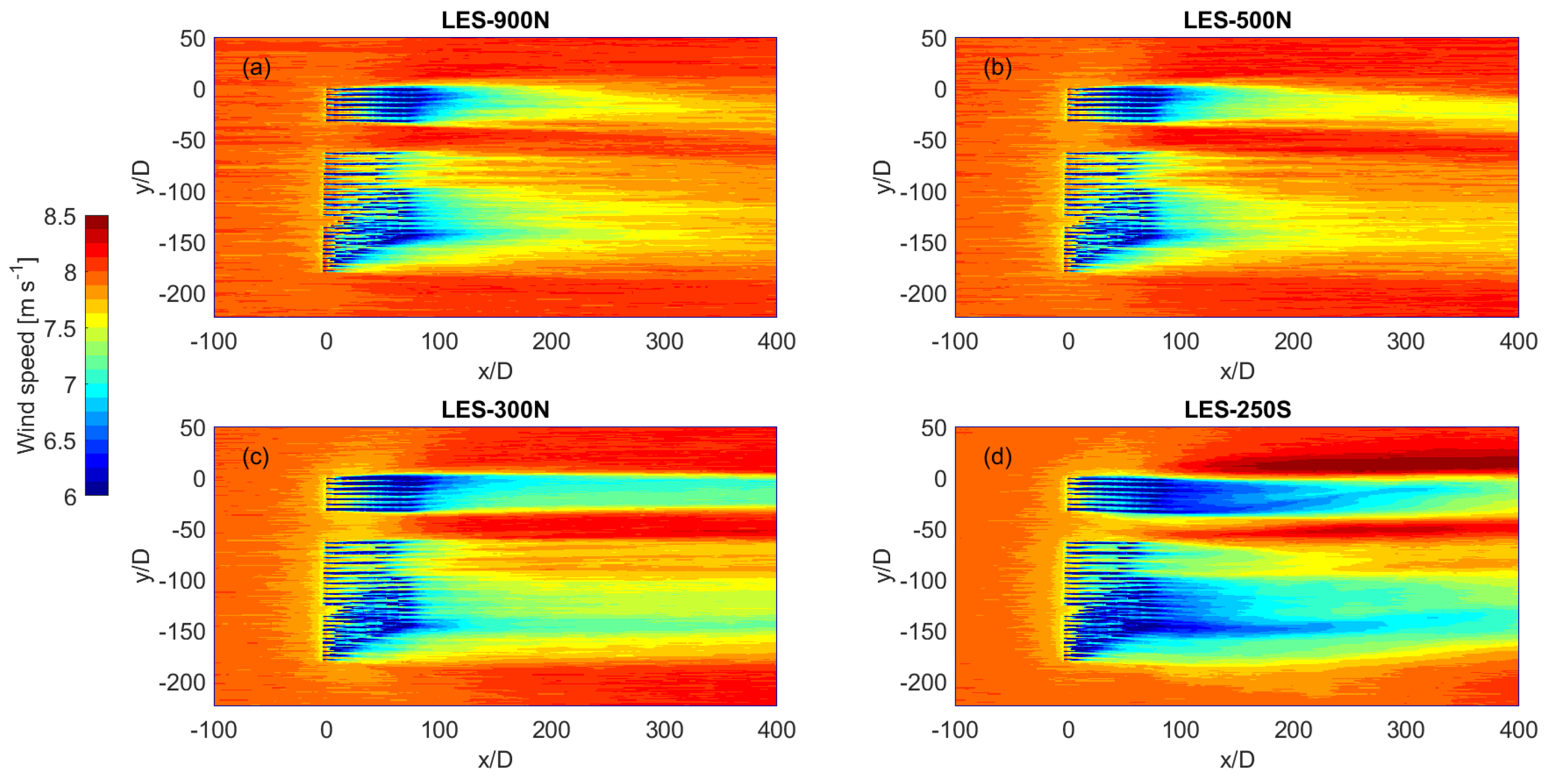
Horizontal cross-sections of the wind speed at hub height in the range 6–8 m s 1 and turbulence intensity, defined as a standard deviation of horizontal wind speed divided by the mean horizontal wind speed (note that only the resolved part of the velocities have been taken into account in the calculation of the turbulence intensity), in the range of 0–10% for neutral (LES-900N, LES-500N and LES-300N) and stable (LES-250S) conditions, are presented in Figure 3 and Figure 4, respectively. Note that LES results presented here are time-averaged during the last 90 min of the main runs. Only results from a part of the total model domain are shown. While the wakes of the individual turbines are often distinguishable many diameters downstream of the wind farm, further downstream, the individual wakes merge into a well-mixed wind farm wake. Upstream of the cluster, the global blockage is evident in all cases, becoming stronger with a decrease in ABL height. A similar blockage flow structure is evident between the LES-300N neutral and LES-250S stable cases, including about 25D in the transverse directions north and south of the cluster, suggesting that the ABL height may be the most important parameter governing the degree of the blockage. However, as the stable case is only slightly stable based on the relatively large Obukhov length (L = 250 m), further stability cases probably need to be conducted to assess the full effect of the stability.
In the stable case, the wind speed reduction in the wakes is more pronounced compared with the neutral LES-300N case, and especially with respect to the two other neutral cases, due to the reduced turbulent mixing and therefore less entrainment of the high-speed flow from above the wind farm [39,40]. Behind the areas more densely populated with wind turbines, the wakes of the LES-500N and LES-900N cases recover to 90% of the freestream wind speed within about 150–200 rotor diameters downstream, while those of LES-300N (neutral) and LES-250S (stable) cases may extend to more than 400 rotor diameters. Directly behind the wind farms, it is clear that the stable case has the largest deficit in wind speed (dark blue areas). Between the wind farms and at the cluster edges, a speed-up in wind speed for the stable case is most evident (than for the neutral cases) from the darker red regions indicating wind speeds > 8 m s 1 . The wakes of the LES-900N and LES-500N cases are slightly steered to the right (looking downstream), while the LES-300N case wakes remain more parallel to the freestream wind direction; there is a clear curvature of the wake structure to the left for the stable case.
There are different competing processes that play a role here. The decrease in the wind speed in the wake leads to a reduction of the Coriolis force at hub height compared to the inflow region. As the Coriolis force is directed to the right of the velocity vector, the reduction of the Coriolis force would support an acceleration of the flow in the northerly direction (as the driving pressure gradient is not affected by the wake). We suspect this process to be dominant in the stable case, as the recovery of the wake is slower than in the neutral cases, resulting in a longer time for the positive v-component (north–south) to develop.
On the other hand, vertical mixing is also reduced in the stable case (compared to the neutral case) and thus the negative v-component from above is not mixed as strongly into the wake region as in the neutral cases. Therefore, our LES results are plausible. Note that Maas and Raasch [26] also saw the deflection of the wakes towards the north in their simulations (see their discussion in Section 3.1.2).
The turbulence intensity in the wake is highest for the neutral LES-900N case, with intensities of 6% extending at least 400 rotor diameters downstream. The exception to this is the narrow region of the elevated turbulence intensity at the northern edge of the ABW wind farm (along the transect y / D 0 ) evident in the other three cases, which seems to increase with decreasing ABL height. These high turbulence streaks have also been observed in airborne measurements at the hub height behind this cluster [41] and can also be observed in SAR images. Likely associated with the intense horizontal wind shear at the farm edges, the turbulence intensity in this region even increases with the increasing distance downstream in contrast to the rest of the wake region, which undergoes an overall reduction in magnitude. Except for the narrow elevated values at the farm edges, the turbulence intensity for the neutral cases tends to return regularly to the freestream magnitude (≈5%). The wake turbulence intensity in the stable case reduces to below-freestream values (≈1%), which would be consistent with the stability being enhanced in the wake because of the reduced wind speed.
Figure 5 presents the percentage wind speed reduction defined as
Δ U ( x / D ) = 100 U U 0 / U 0
as a function of the normalized distance x / D , where the distance x is in the wind direction at hub height, D is the rotor diameter, U is the hub height free wind speed, and U 0 is the upstream hub height wind speed. Note that the parameter ‘wind speed reduction’ is a negative value with respect to the freestream wind speed in the wake, while the term ‘wake recovery’ describes the tendency of the wind speed to return to the freestream wind speed downstream of a wind farm, so that a wind speed reduction of 5 % is a wake recovery of 95%.
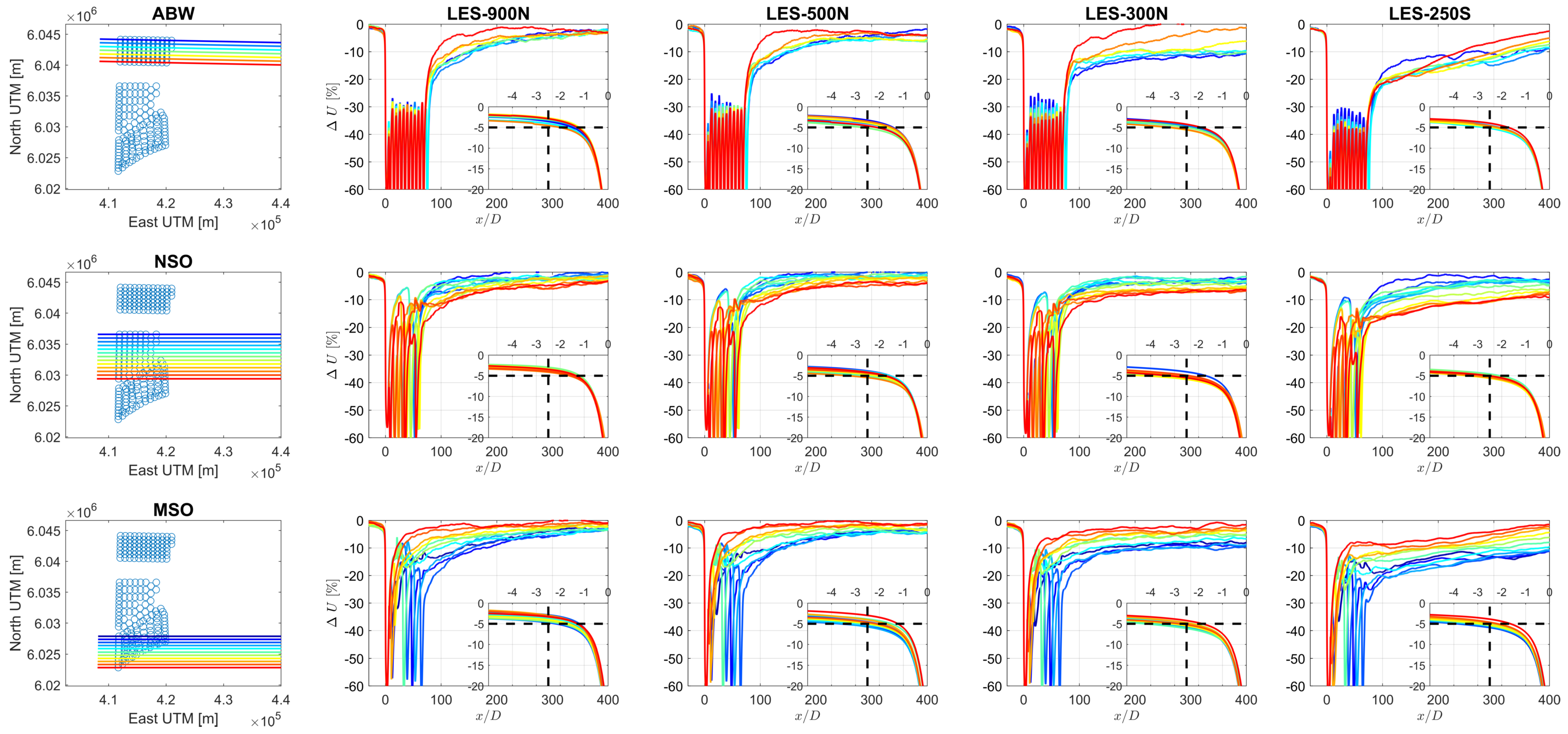
The first column of panels in Figure 5 illustrates the positions to which the curves in the other panels pertain based on the line coloring. The wind speed reduction for the ABW, NSO and MSO wind farms are shown in the top, middle and bottom rows of panels, respectively. The neutral LES cases LES-900N, LES-500N and LES-300N are shown in the columns 2–4, and the stable case in the right-most column 5. Each main panel in columns 2–5 shows the wind speed reduction in the range x / D = 30 –400 and each inset shows the induction zone in the range x / D = 5 –0, where 0 is the position of the first row of wind turbines (there is a curve for each first-row wind turbine). For example, the blue curves in the top row correspond to the wind speed reduction along a line through the uppermost row of the ABW wind farm, where x / D = 0 is the location of the first turbine in that row.
In general, the wakes and induction are stronger and the wind speed reduction becomes more negative when viewing the panels from left to right. The wakes and induction are generally stronger in the ABW wind farm with more densely packed wind turbines compared with the NSO and MSO farms. The NSO wind farm is more sparsely populated than the ABW wind farm, which leads to a quicker recovery of the wind speed to freestream values. The MSO wind turbines are more irregularly spaced, which results in a greater variation in wind speed reduction with the position, as observed by the spread of curves in the bottom row of panels in Figure 5.
The tightly spaced and more regular ABW wind turbines produce a similar wind speed recovery at all positions for the neutral LES-900N and LES-500N cases, with both recovering to 95% of the freestream wind speed at about 200 rotor diameters downstream. The neutral LES-300N wake recovers to only 90% of the freestream wind speed within 400 rotor diameters downstream, except for the red curve representing the wind speed recovery along the turbines nearest the Kaskasi gap (narrow area between ABW and NSO wind farms), whose relatively greater recovery is the result of a slight narrowing of the wake for this case behind the ABW wind farm, in contrast to the wake spreading for the LES-900N and LES-500N cases (c.f. Figure 3). This would be consistent with the slight speed-up detected outside the wakes.
More complex is the stable case where the wind speed reduction of the most northern row reaches a maximum before integrating into a recovery in rough accordance with the other curves; this row seems to benefit from a wake narrowing and speed-up to the north (c.f. Figure 3). For the ABW farm, the magnitude of the induction effect upstream increases, but the spread of curves decreases, with a decreasing ABL height and increasing stability, ranging from 2.5% to 6% at 2.5D upstream ( x / D = 2.5 in Figure 5).
The wake recovery downstream of the NSO wind farm reaches approximately 95% within about 100 rotor diameters, depending on the case and the turbine row. The LES-500N case may even recover slightly quicker than the LES-900N case, and there is even a speed-up evident in the blue LES-500N curve, representing the turbine row nearest the Kaskasi Gap, and thus sampling the elevated wind speed there (c.f. Figure 3). Although the wake recovery in the LES-300N case recovers relatively quickly, the wind speed reduction does not converge to 0% but to somewhere between 0% and −10% depending on the row, with the ‘warmer’ colors toward −10%, as these also represent the sampling of the northern rear of the MSO wind farm. The wake recovery in stable conditions appears more complete for the more northern rows in the NSO farm (‘cooler’ colors), which could partly be attributed to the influence of the speed-up within the Kaskasi Gap impeding on the wake flow (c.f. Figure 3). The recovery is only 90% complete within 400 rotor diameters for the red curves that also sample part of the MSO wind farm. The difference in induction between the cases varies similarly with the ABW farm, varying from 2.5% at 2.5D for the LES-900N case to 6% for the stable case; there is slightly more spread compared with the ABW wind farm for stable conditions.
The wake recovery for the MSO wind farm follows the expected pattern considering the wind farm width, which increases in extension from the south to north for flow from the west. The red curve in Figure 5 represents the wind speed reduction from a single turbine under the influence of the wider wind farm, e.g., from a global blockage. This single southern wind turbine has a wake that recovers to 95% of the freestream wind speed within the first 50D downstream for all neutral cases. For the stable case, the single-turbine wake recovers quickly, which is initially consistent with the neutral cases until 50D, with the recovery slowing thereafter at a rate almost consistent with the rest of the wind farm. At 400D downstream, the entire wake recovers to 95% of the freestream wind speed for the LES-900N and LES-500N cases, but for the LES-300N case, there is a convergence to wind speed reductions of between −15 and 0% depending on the row. For the stable case, the convergence is still ongoing at 400D downstream, which is related to the curvature of the wake towards the north (c.f. Figure 3d). The induction for the single-turbine case for a 840 m ABL height (LES-900N case) corresponds to the magnitude of about 0.5–1% at 2.5 D , which is what one expects for a single isolated turbine [40,42].
As the ABL height decreases for neutral conditions or as the stability increases, the becomes more significant and the spread between the different turbines also increases, with the most induction found for the northern-most wind turbine in the MSO wind farm.

5.1.2. Deep-Array Wake Model (DAWM) Simulations

Figure 6c presents the horizontal cross-sections of the DAWM/EV/RHB wind speed compared with the LES-900N neutral LES (Figure 6a). The downstream expansion rate of the DAWM wind farm wakes is probably too excessive compared with the LES results. A couple of dark-blue patches in the direct near-wake regions of the ABW and MSO wind farms representing wind speeds of ≈6 m s 1 are underestimated by the DAWM model. Nonetheless, the overall recovery of wind speeds from 7 m s 1 at 100D to 7.5 m s 1 at 250D corresponds broadly with the LES results.
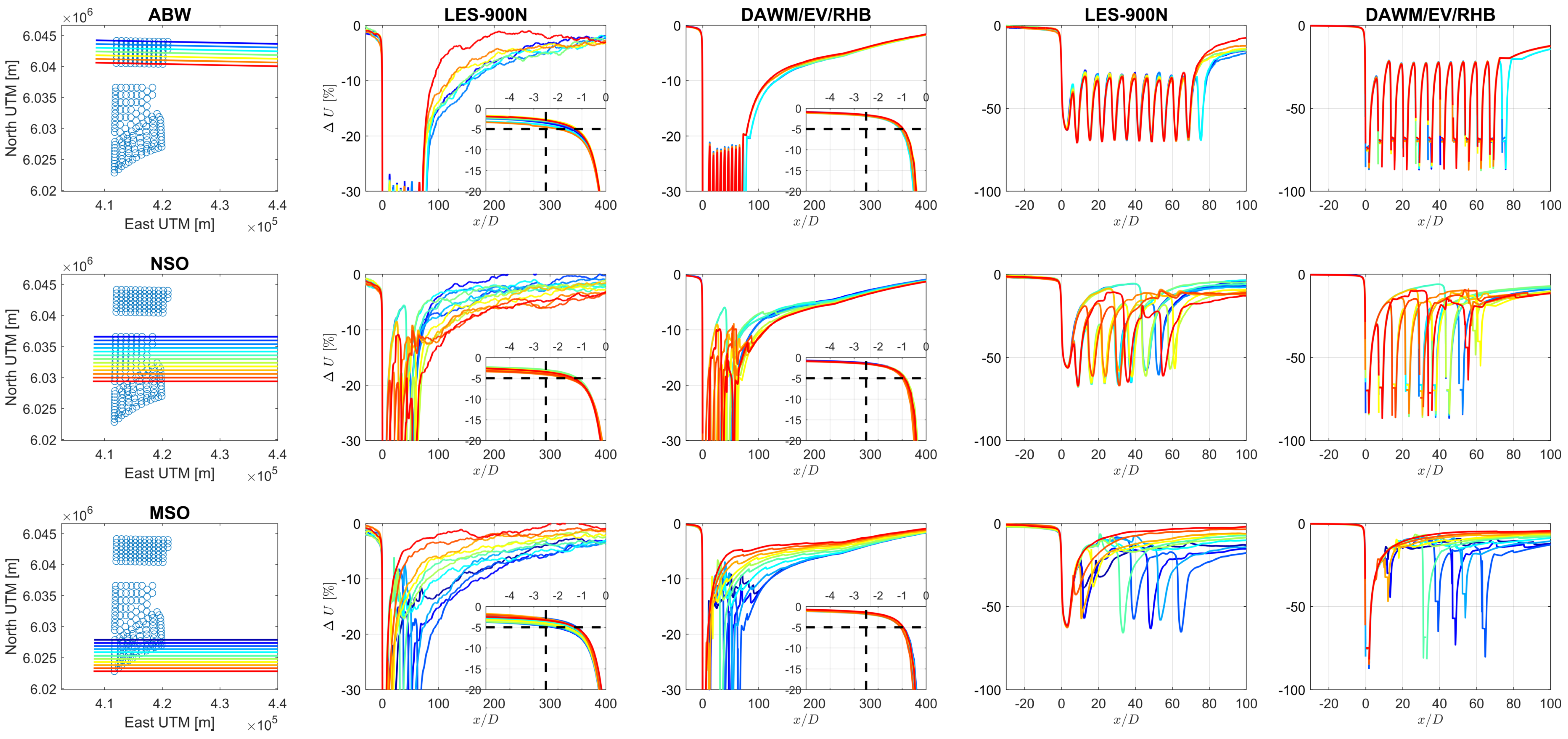
Figure 7 presents the DAWM/EV/RHB results as lines through each row of wind turbines based on the front row equivalently to that displayed above in Figure 5. For reference, the 900 m neutral LES case is shown in the first and third column panels, which is the closest LES simulation to the standard configuration of the DAWM model. Note that the panels in the final two columns have had their axes adjusted to magnify the EV wake region directly within the wind farms. The DAWM model captures the overall magnitude of the far-field wake, with all curves merging to a single curve. Therefore, the wake spreading suggested by the LES results is not completely reproduced by the DAWM. For the ABW wind farm, the LES-900N results give a wind speed reduction of ≈−15% and ≈−7% at 100D and 200D, respectively, compared with 13 % and 6 % for the DAWM model. Downstream of the NSO wind farm, the DAWM results sit at the lower bound of the spread in the LES curves, amounting to wind speed reductions of 10 % and 6 % at 100D and 200D, respectively. For the MSO wind farm, the DAWM results (≈−5% at 200D) are within the spread of the LES results ( 1 to 8 % at 200D). In the near-field wake region (0–100D), the LES results reveal a wind speed reduction of a bit less than 50%. The DAWM absolute wind speed reduction is slightly higher because of the higher resolution (infinite) of an analytical model compared with the 10-m resolution of the LES model. The global blockage is slightly underestimated by the RHB model (≈−1.5% at 2.5D), which the LES results indicate to reach up to 3.5 % at 2.5D. Appendix A presents a further comparison between the three implemented induction models in Openwind and the LES output.

5.1.3. Array-Stability Wake Model (ASM) Simulations

Figure 6 compares horizontal cross-sections of the wind speed at hub height according to the ASM model (d) with the stable LES ( L = 250 m) results (b).
The ASM and LES-250 wake wind speeds broadly match directly downstream from the ABW wind farm. The extended blue streak of the wake behind the northern part of the MSO wind farm in the LES results has not been captured well in the ASM results. In contrast, the southern part of the MSO wind farm looks to have been simulated better with respect to the LES results.
The global blockage produced by the ASM simulation is qualitatively consistent with the LES results. No speed-up can be reproduced in the ASM approach, such as that found in the Kaskasi Gap in the LES results, since the ASM accounts for only the wind farm drag and wind speed recovery.
Similar to Figure 5 and Figure 7, wind speed reduction profiles are displayed in Figure 8, where the ASM results are presented in the third and fifth columns and the LES-250S results in the second and fourth columns. At x / D = 100 , the wind speed reductions are 12 % and 20 % for the ABW wind farm for the ASM and LES results, respectively, which reflects the underestimated ASM wake there. At the same position for the NSO wind farm, the reductions are 10 % and 5 to 15 % for the ASM and LES results, respectively. For both the ABW and NSO wind farms, the induction at approximately 2.5D is about 2.5% less in the ASM model compared with the LES results, which give about a 5% reduction at this upstream distance; the induction is more consistent for the MSO wind farm.

5.2. Wind Farm Results

Measurements of the individual wind turbine power provide a real-world check of the plausibility of the models (both LES and OpenWind), although much pre-processing of such measurements is required, as is now briefly described. Approximately five years of 10-min-averaged Supervisory Control and Data Acquisition (SCADA) data from both the ABW and NSO wind farms are considered. From those five years, only periods of normal operating conditions are considered, which means curtailments, shutdowns, and other alarms are filtered from consideration for each wind turbine. Moreover, poor quality data, such as that due to negative wind speeds or data dropouts, are also removed from the SCADA dataset. In the end, a very small data set is considered, where the number of SCADA 10-min data (min, max) for the wind turbines used are given in Table 4.
The resulting quality-controlled SCADA dataset is then filtered for westerly wind directions and 8 m s 1 wind speeds. Since a reference meteorological tower is not available, the north-western-most wind turbine of each farm is used as a reference for both wind speed and direction, assuming this turbine is the least affected by flow distortion. Relatively conservative wind speed and direction bins of 7–9 m s 1 and 260–280° are used to ensure a sufficient amount of data for each case listed in Table 3. The boundary-layer height and atmospheric stability as calculated by the Weather Research and Forecasting (WRF) model for the entire five-year period are used to match the SCADA data with the LES cases. Boundary-layer-height bin widths of 800–1000 m, 400–600 m and 200–400 m, are used to match the SCADA data to the 900N, 500N and 300N cases. The Monin–Obukhov stability parameter ( z / L ) is restricted to an absolute value of 0.5 in the neutral cases and >0.5 for the stable case of 250S, which also has a boundary-layer-height bin width of 200–400 m.
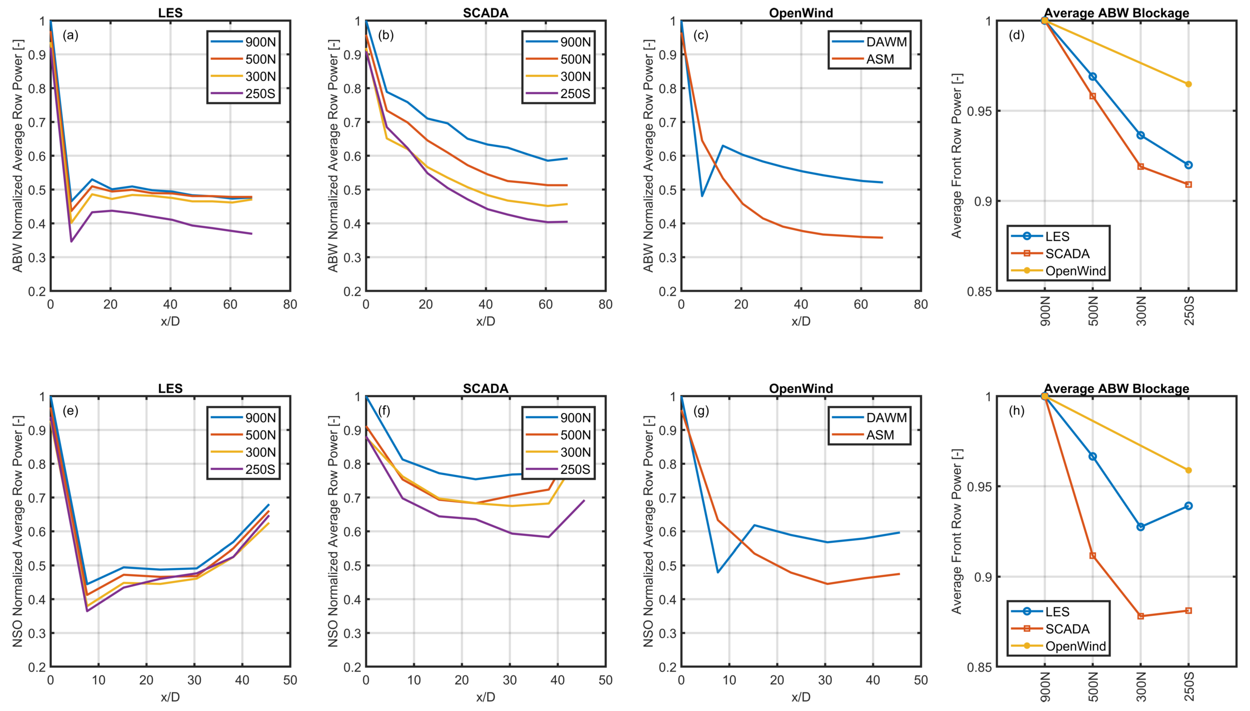
To provide an overall comparison of model results through the ABW and NSO wind farms, Figure 9 presents the average power through a “row” aligned in the north–south direction for each farm—panels a–c show the model and SCADA results for the ABW wind farm and panels e–g for the NSO farm. The power along each of these “rows” is then normalized by the front or most western north–south row for the 900N case, and the average downstream position x for each north–south row with respect to the western row is normalized by the rotor diameter D to provide the x-coordinates. Figure 9a–c show the LES, SCADA and OpenWind results for the ABW farm and Figure 9e–g for the NSO farm, respectively. Each case (900N, 500N, 300N and 250S) is indicated in the legend. For the OpenWind results, the DAWM and ASM results correspond roughly to the 900N and 250S LES cases. The blockage effect for each wind farm is plotted in Figure 9d,h, showing the average front row power with respect to the 900N case for the LES and OpenWind models, and the SCADA dataset.
Figure 9a,e show a small reduction in power for a reduction in boundary-layer height and an increase in atmospheric stability, for both wind farms. The SCADA results presented in Figure 9b,f tend to show a more significant boundary-layer height and atmospheric stability dependence. The qualitative shape of the SCADA curves is also different with respect to the LES curves, particularly for the ABW wind farm. Note, however, that the LES data represent highly idealized conditions consisting of uniform north–south inflow and a perfect alignment of turbines to the west, which almost never happens in practice; turbines are often pointing ±15° away from the incoming flow. With that caveat, the shape of the DAWM curves follow the idealized LES conditions while the ASM/TurboPark curve more reflects the SCADA data. Assuming the DAWM approach simulates idealized neutral conditions, the ASM approach may well be able to model the slightly stable conditions based on the reduced power expected in such conditions.
The blockage curves based on the average front row power shown in Figure 9d,h for each wind farm would suggest a greater reduction in power with decreasing boundary-layer height. Interestingly, for the NSO wind farm, both the LES and SCADA data show slightly more power in the stable 250S case than for the 300N case. The ASM blockage may have to be strengthened with respect to the neutral DAWM approach to reflect the front-row power reduction in the LES and SCADA datasets. Further investigations with more stability cases will be performed in the future.

6. Discussion

Four LES runs for an operational wind farm cluster layout and idealized, spatially homogeneous inflow conditions (8 m s 1 and 270°) have been performed and used as references with which to assess a fast engineering model. However, even for these seemingly idealized conditions, there are further complexities which complicate a hard and fast reference on which to base engineering models. For example, the boundary-layer height, which is generally not accounted for in engineering models and rarely measured, has an obvious effect on the wake strength according to the LES results, with lower boundary-layer heights tending to restrict the flow recovery further downstream as well as increase the global blockage effect. Atmospheric stability is a well-known complication that is at the same time correlated with the boundary-layer height, but even with LES, only a weakly stable LES run may be considered because of the numerical challenges associated with the limitations of subgrid-scale models in LES stably stratified boundary layers. Moreover, due to the large domain needed to perform the LES simulations and the small resolution of the grid used, only a few cases are feasible, which means a judicious selection of the important flow features from a few selected cases is required.
Considering the strengths and weaknesses of the LES approach, one can conclude that LES represents an excellent starting point on which to investigate cluster flow phenomena relevant for engineering models, but some other source such as SCADA data should probably be used to contextualize the LES results in terms of the real-world wind power. For example, LES assumes not only a ’perfect’ homogeneous flow but also a homogeneous turbine behavior, which is also an idealization. Therefore, the comparison in Figure 9b would suggest that the LES wake strengths presented here are the maximum to be expected given a perfectly operational wind farm (e.g., no nacelle misalignment), and the seemingly ’conservative’ nature of engineering models such as DAWM are justified even if they do not perfectly match the LES results. At the same time, the new ASM approach can probably be improved and optimized based on a more comprehensive (including stability) assessment of SCADA data from multiple wind farms and flow conditions.

7. Conclusions

Large-eddy simulations of the N-4 wind farm cluster consisting of the ABW, NSO and MSO wind farms in the North Sea have been performed to provide an accurate, albeit idealized, reference as to the strength of the wind speed reduction (or speed-up) upstream, through and downstream in neutral and stable conditions and three boundary-layer heights. The wake and induction strength generally increase for lower boundary-layer heights, lower turbine spacing and for stable conditions. The bulk structure of the flow is able to be reproduced by both the deep-array wake and array-stability models, depending on the desired application (e.g., stability), although the finer details of the LES results are unlikely to be reproduced simply by engineering methods, such as the speed-up detected in the ’Kaskasi Gap’ between the ABW and NSO wind farms. Moreover, the engineering models considered here may be conservative with respect to the LES results, but justified based on the limited SCADA data considered.
In neutral conditions, the DAWM set-up is able to capture the main flow aspects with respect to the LES results, but needs to be replaced by the ASM set-up in order to reproduce the more intense wake and blockage effects found in stable conditions. The ASM approach in turn does not currently take into account the boundary-layer height, for which more advanced methods may have to be developed. The ASM approach could conceivably be made boundary-layer-height dependent by adjusting the Δ z scale, whereas here we have the pragmatic decision to keep it constant.
Further development work will be performed in real conditions by comparing Openwind’s newly developed methods with SCADA data for different flow scenarios and wind farm layouts.

Author Contributions

Both B.C. and R.F. wrote the manuscript and evaluated and prepared most of the figures. G.S. performed the LES simulations. N.R. implemented the new parameterizations in Openwind. All authors contributed intensively to an internal review. All authors have read and agreed to the published version of the manuscript.

Funding

This research has been supported by the X-Wakes project, funded by the Federal Ministry for Economic Affairs and Climate Action (BMWK) (grant no. FKZ 03EE3008 (A-G)). LES simulation computing resources were partly provided by the North-German Supercomputing Alliance (HLRN).

Data Availability Statement

The raw/processed data required to reproduce the above findings cannot be shared at this time as the data also forms part of an ongoing project.

Acknowledgments

The authors would like to thank the Publication Fund of the TU Braunschweig for financially supporting the freely accessible publication of this article. The authors would like to thank the RWE team and especially Sam Williams from RWE for sharing the SCADA data.

Conflicts of Interest

The authors declare no conflict of interest.

Appendix A. Induction Model Performance in Openwind
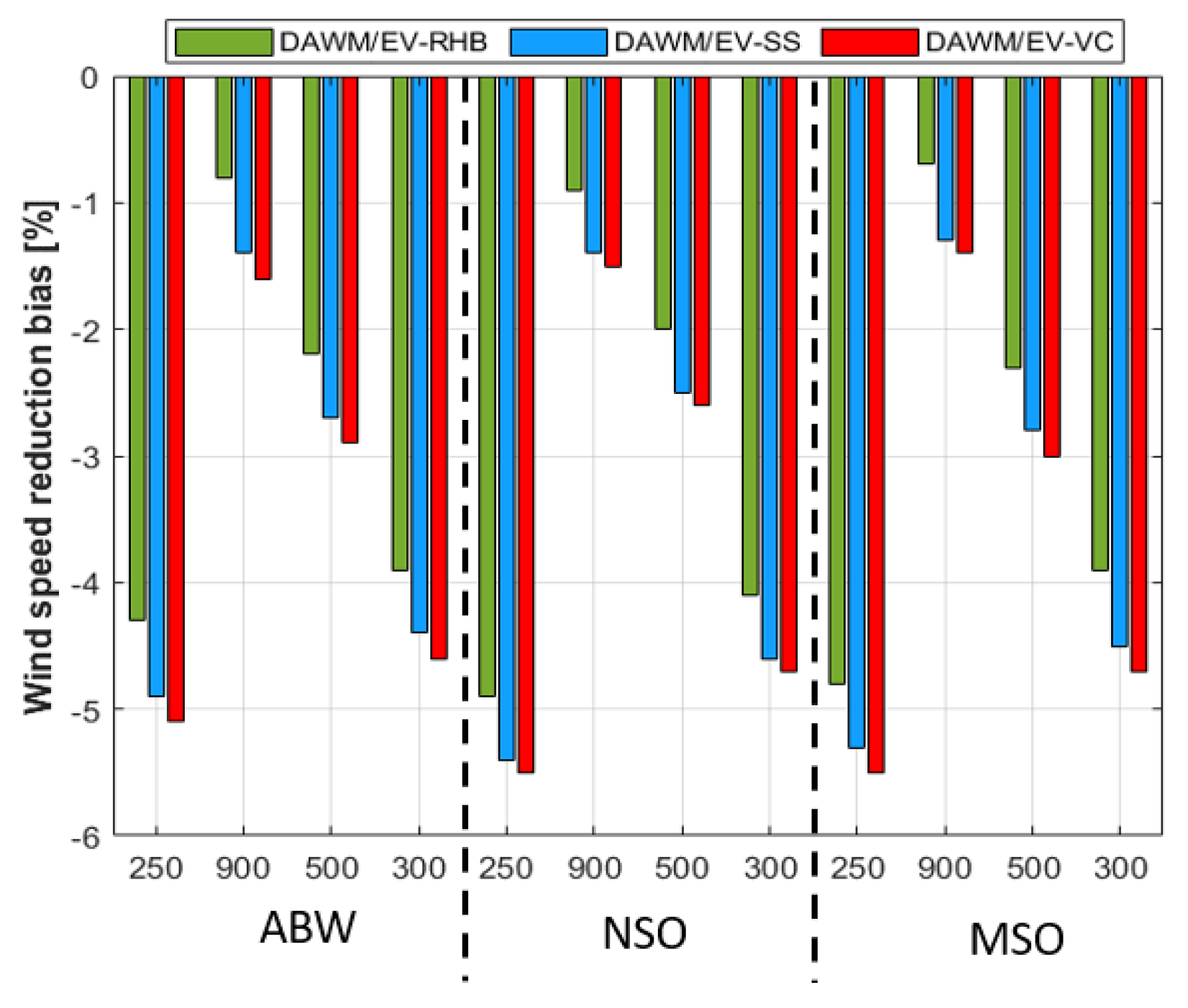
Figure A1 shows the average percentage wind speed reduction at 2.5 D upstream of each N-4 wind farm between the LESs and three of the most recent induction models proposed in the literature (namely, the Self-similar (SS), Vortex Cylinder (VC) and Rankine-Half Body (RHB) models). Since these models are based on a single wind turbine induction model, the cumulative effect of all wind turbines in a series is linearly superimposed. In these induction models, the upstream wind speed along the rotor axis is a function of the rotor induction factor ( a = a ( C T ) ), the upstream position in the flow direction (zero at the turbine and negative upwind) and the rotor diameter D.
Figure A1. Averaged percentage of wind speed reduction bias (LES-Induction model) at 2.5 D upstream of each N-4 wind farms and for each induction model implemented in Openwind and coupled with DAWM the model.
Energies 16 02949 g0a1
Figure A1 shows that the differences between the individual induction models for each case are “very similar” (1%), with the RHB model being the closest to the LES outputs. In general, all models underestimate the wind speed reduction (or deficit) upstream of each wind farm, with the bias increasing (from around 1% to 5%) with decreasing ABL height and increasing stability at a distance of 2.5 D . A similar finding was made by [27], who compared these models with neutral LESs of two idealized wind farms. It was found that these models correctly describe the induction generated by a single wind turbine, but are not transferable when these models are linearly superimposed to describe the upstream flow. The same is found for the ABL height.

Appendix B. Array-Stability Model (ASM)

The stability-dependent wake model proposed by [20,43] is adapted for the OpenWind suite to account for stability-dependent wake and induction effects to be used in combination with a wind turbine wake model such as the Ainslie [10] or Bastankhah and Porté-Agel [11] models. Firstly, to account for far-field wakes, assume that the temporal evolution of the wind speed within the wake is only dependent on the vertical momentum exchange within the wake of a wind farm, then
U w t = u w ¯ z ,
where U w is the wind speed within the wake, t is the time, z is the height above the surface and u w ¯ is the vertical kinematic momentum flux [m 2 s 2 ]. A bulk parametrization for the kinematic momentum flux u w ¯ may be written in terms of an exchange coefficient or eddy viscosity K [m 2 s 1 ] by
u w ¯ = K U U w Δ z 2 ,
where U is the freestream wind speed, Δ z 2 (= D) is the vertical separation between the freestream flow and the wake flow, and K is an exchange coefficient describing the efficiency of the momentum exchange between the freestream flow and the wake flow. Solving for (A1) and (A2) U w gives the wind speed ratio in the wake as
R U = U w U = 1 + U 0 U 1 exp α x ,
where the inverse wind speed recovery scale α = K / Δ z 2 2 U w [m 1 ], and x is the downstream distance. Close to the surface, the exchange coefficient
K = κ u * h ϕ ,
where κ is the von Karman constant, u * is the friction velocity, h is the wind turbine hub height and the dimensionless wind shear
Φ = κ z u * U z = f ζ ,
where f is a function dependent only on the Monin–Obukhov similarity parameter ζ . The friction velocity can be estimated from the logarithmic freestream wind speed profile as
U = u * κ ln z z 0 Ψ ζ ,
where z 0 is the roughness length, and Ψ is the stability correction for varying ζ .
Next, the wind speed distribution within the wind farm U 0 can be estimated using the the wind speed ratio behind the wind farm [20,43,44] as
R U 0 = U 0 U = h + Δ z 1 Δ z 1 I u + Φ m κ 2 C d h + Δ z 1 Δ z 1 I u + Φ m κ 2 C t , e f f ,
where Δ z 1 (= 0.05 D ) is a length scale analogous to Δ z 2 in Equation (A2) but for within the wind farm, and I u is the ambient turbulence intensity. The effective wind farm drag coefficient throughout the wind farm is
C t , e f f ( x , y ) = π 8 c t ( x , y ) + C d ,
which the sum of the freestream surface drag C d u * 2 / U 2 , and the area-distributed wind farm thrust coefficient c t ( x , y ) .
Finally, and this step accounts for both the thrust drag downstream while simulating the induction upstream, c t ( x , y ) is the wind turbine thrust coefficient C T for each wind turbine distributed over an area using a skew-Gaussian distribution defined by a function of width σ = 9 D in the x direction (streamwise), and σ = 3 D in the y (lateral) direction) and a skewness (=2). The skewness biases the function toward the downstream of the wind turbine. This process simulates the wind speed reduction upstream due to the induction through the calculation of R U 0 in Equation (A7) (the value of C t , e f f ( x , y ) is small but non-zero upstream). The roughness drag coefficient is estimated from the logarithmic wind speed profile as
C d = κ 2 ln z z 0 2 .

References

  1. Allaerts, D.; Meyers, J. Gravity Waves and Wind-Farm Efficiency in Neutral and Stable Conditions. Bound.-Layer Meteorol. 2018, 166, 990–1028. [Google Scholar] [CrossRef] [Green Version]
  2. Cañadillas, B.; Foreman, R.; Barth, V.; Siedersleben, S.; Lampert, A.; Platis, A.; Djath, B.; Schulz-Stellenfleth, J.; Bange, J.; Emeis, S.; et al. Offshore wind farm wake recovery: Airborne measurements and its representation in engineering models. Wind Energy 2020, 23, 1249–1265. [Google Scholar] [CrossRef]
  3. Platis, A.; Bange, J.; Bärfuss, K.; Cañadillas, B.; Hundhausen, M.; Djath, B.; Lampert, A.; Schulz-Stellenfleth, J.; Siedersleben, S.; Neumann, T.; et al. Long-range modifications of the wind field by offshore wind parks – results of the project WIPAFF. Meteorol. Z. 2020, 29, 355–376. [Google Scholar] [CrossRef]
  4. Nygaard, N.G.; Steen, S.T.; Poulsen, L.; Pedersen, J.G. Modelling cluster wakes and wind farm blockage. J. Phys. Conf. Ser. 2020, 1618, 062072. [Google Scholar] [CrossRef]
  5. UL-International. Openwind User Manual; Technical Report; AWS Truepower, LLC: Albany, NY, USA, 2020. [Google Scholar]
  6. Brower, M.; Robinson, N. The OpenWind Deep-Array Wake Model: Development and Validation; Technical Report; AWS Truepower: Albany, NY, USA, 2012. [Google Scholar]
  7. Frandsen, S.T. Turbulence and Turbulence-Generated Structural Loading in Wind Turbine Clusters; Risø National Laboratory: Roskilde, Denmark, 2007. [Google Scholar]
  8. Beaucage, P.; Robinson, N.; Brower, M.; Alonge, C. Overview of six commercial and research wake models for large offshore wind farms. In Proceedings of the EWEA 2012, Copenhagen, Denmark, 16–19 April 2012. [Google Scholar]
  9. Jensen, N. A Note on Wind Generator Interaction; Risø National Laboratory: Roskilde, Denmark, 1983. [Google Scholar]
  10. Ainslie, J. Calculating the flowfield in the wake of wind turbines. J. Wind. Eng. Ind. Aerodyn. 1988, 27, 213–224. [Google Scholar] [CrossRef]
  11. Bastankhah, M.; Porté-Agel, F. A new analytical model for wind-turbine wakes. Renew. Energy 2014, 70, 116–123. [Google Scholar] [CrossRef]
  12. Porté-Agel, F.; Bastankhah, M.; Shamsoddin, S. Wind-Turbine and Wind-Farm Flows: A Review. Bound.-Layer Meteorol. 2020, 174, 1–59. [Google Scholar] [CrossRef] [Green Version]
  13. Branlard, E.; Gaunaa, M. Cylindrical vortex wake model: Right cylinder. Wind Energy 2015, 18, 1973–1987. [Google Scholar] [CrossRef]
  14. Troldborg, N.; Meyer Forsting, A. A simple model of the wind turbine induction zone derived from numerical simulations. Wind Energy 2017, 20, 2011–2020. [Google Scholar] [CrossRef]
  15. Gribben, B.J.; Hawkes, G.S. A Potential Flow Model for Wind Turbine Induction and Wind Farm Blockage; Technical Report; Frazer-Nash Consultancy: Surrey, UK, 2019. [Google Scholar]
  16. Allaerts, D.; Meyers, J. Boundary-layer development and gravity waves in conventionally neutral wind farms. J. Fluid Mech. 2017, 814, 95–130. [Google Scholar] [CrossRef] [Green Version]
  17. Allaerts, D.; Meyers, J. Sensitivity and feedback of wind-farm-induced gravity waves. J. Fluid Mech. 2019, 862, 990–1028. [Google Scholar] [CrossRef]
  18. Lanzilao, L.; Meyers, J. Set-point optimization in wind farms to mitigate effects of flow blockage induced by atmospheric gravity waves. Wind. Energy Sci. 2021, 6, 247–271. [Google Scholar] [CrossRef]
  19. Bleeg, J.; Purcell, M.; Ruisi, R.; Traiger, E. Wind Farm Blockage and the Consequences of Neglecting Its Impact on Energy Production. Energies 2018, 11, 1609. [Google Scholar] [CrossRef] [Green Version]
  20. Emeis, S. Wind Energy Meteorology: Atmospheric Physics for Wind Power Generation; Springer: Berlin/Heidelberg, Germany, 2018. [Google Scholar]
  21. Maronga, B.; Gryschka, M.; Heinze, R.; Hoffmann, F.; Kanani-Sühring, F.; Keck, M.; Ketelsen, K.; Letzel, M.O.; Sühring, M.; Raasch, S. The Parallelized Large-Eddy Simulation Model (PALM) version 4.0 for atmospheric and oceanic flows: Model formulation, recent developments, and future perspectives. Geosci. Model Dev. 2015, 8, 2515–2551. [Google Scholar] [CrossRef] [Green Version]
  22. Maronga, B.; Banzhaf, S.; Burmeister, C.; Esch, T.; Forkel, R.; Fröhlich, D.; Fuka, V.; Gehrke, K.F.; Geletič, J.; Giersch, S.; et al. Overview of the PALM model system 6.0. Geosci. Model Dev. 2020, 13, 1335–1372. [Google Scholar] [CrossRef]
  23. Witha, B.; Steinfeld, G.; Dörenkämper, M.; Heinemann, D. Large-eddy simulation of multiple wakes in offshore wind farms. J. Phys. Conf. Ser. 2014, 555, 012108. [Google Scholar] [CrossRef] [Green Version]
  24. Steinfeld, G.; Witha, B.; Dörenkämper, M.; Gryschka, M. Hochauflösende Large-Eddy-Simulationen zur Untersuchung der Strömungsverhältnisse in Offshore-Windparks. Promet-Meteorol. Fortbild. 2016, 39, 163–180. [Google Scholar]
  25. Vollmer, L.; Steinfeld, G.; Heinemann, D.; Kühn, M. Estimating the wake deflection downstream of a wind turbine in different atmospheric stabilities: An LES study. Wind. Energy Sci. 2016, 1, 129–141. [Google Scholar] [CrossRef] [Green Version]
  26. Maas, O.; Raasch, S. Wake properties and power output of very large wind farms for different meteorological conditions and turbine spacings: A large-eddy simulation case study for the German Bight. Wind. Energy Sci. 2022, 7, 715–739. [Google Scholar] [CrossRef]
  27. Centurelli, G.; Vollmer, L.; Schmidt, J.; Dörenkämper, M.; Schröder, M.; Lukassen, L.; Peinke, J. Evaluating Global Blockage engineering parametrizations with LES. J. Phys. Conf. Ser. 2021, 1934, 012021. [Google Scholar] [CrossRef]
  28. Stieren, A.; Stevens, R.J.A.M. Evaluating wind farm wakes in large eddy simulations and engineering models. J. Phys. Conf. Ser. 2021, 1934, 012018. [Google Scholar] [CrossRef]
  29. Zhan, L.; Letizia, S.; Iungo, G. Optimal tuning of engineering wake models through lidar measurements. Wind. Energy Sci. 2020, 5, 1601–1622. [Google Scholar] [CrossRef]
  30. Grønnegaard Pedersen, J.; Svensson, E.; Poulsen, L.; Gayle Nygaard, N. Turbulence Optimized Park model with Gaussian wake profile. J. Phys. Conf. Ser. 2022, 2265, 022063. [Google Scholar] [CrossRef]
  31. Saiki, E.; Moeng, C.; Sullivan, P. Large-Eddy Simulation Of The Stably Stratified Planetary Boundary Layer. Bound.-Layer Meteorol. 2000, 95, 1–30. [Google Scholar] [CrossRef] [Green Version]
  32. Dai, Y.; Basu, S.; Maronga, B.; de Roode, S. Addressing the Grid-Size Sensitivity Issue in Large-Eddy Simulations of Stable Boundary Layers. Bound.-Layer Meteorol. 2020, 178, 63–89. [Google Scholar] [CrossRef]
  33. Wu, Y.T.; Porte-Agel, F. Large-Eddy Simulation of Wind-Turbine Wakes: Evaluation of Turbine Parametrisations. Bound.-Layer Meteorol. 2011, 138, 345–366. [Google Scholar] [CrossRef]
  34. Abkar, M. Impact of Subgrid-Scale Modeling in Actuator-Line Based Large-Eddy Simulation of Vertical-Axis Wind Turbine Wakes. Atmosphere 2018, 9, 257. [Google Scholar] [CrossRef] [Green Version]
  35. Asmuth, H.; Diaz, G.P.N.; Madsen, H.A.; Branlard, E.; Forsting, A.R.M.; Nilsson, K.; Jonkman, J.; Ivanell, S. Wind turbine response in waked inflow: A modelling benchmark against full-scale measurements. Renew. Energy 2022, 191, 868–887. [Google Scholar] [CrossRef]
  36. Dar, A.S.; Berg, J.; Troldborg, N.; Patton, E.G. On the self-similarity of wind turbine wakes in a complex terrain using large eddy simulation. Wind. Energy Sci. 2019, 4, 633–644. [Google Scholar] [CrossRef] [Green Version]
  37. Pena, A.; Mirocha, J.D.; van der Laan, M.P. Evaluation of the Fitch Wind-Farm Wake Parameterization with Large-Eddy Simulations of Wakes Using the Weather Research and Forecasting Model. Mon. Weather. Rev. 2022, 150, 3051–3064. [Google Scholar] [CrossRef]
  38. Williamson, J. Low-storage runge-kutta schemes. J. Comput. Phys. 1980, 35, 48–56. [Google Scholar] [CrossRef]
  39. Magnusson, M.; Smedman, A.S. Air flow behind wind turbines. J. Wind. Eng. Ind. Aerodyn. 1999, 80, 169–189. [Google Scholar] [CrossRef]
  40. Strickland, J. Modeling Wakes and Blockage in Large-Scale Wind Farms. Ph.D. Thesis, University of Twente, Enschede, The Netherlands, 2021. [Google Scholar] [CrossRef]
  41. Platis, A.; Siedersleben, S.; Bange, J.; Lampert, A.; Bärfuss, K.; Hankers, R.; Cañadillas, B.; Foreman, R.; Schulz-Stellenfleth, J.; Djath, B.; et al. First in situ evidence of wakes in the far field behind offshore wind farms. Sci. Rep. 2018, 8, 2163. [Google Scholar] [CrossRef] [PubMed] [Green Version]
  42. Medici, D.; Ivanell, S.; Dahlberg, J.; Alfredsson, P.H. The upstream flow of a wind turbine: Blockage effect. Wind Energy 2011, 14, 691–697. [Google Scholar] [CrossRef]
  43. Emeis, S. A simple analytical wind park model considering atmospheric stability. Wind Energy 2010, 13, 459–469. [Google Scholar] [CrossRef]
  44. Frandsen, S. On the wind speed reduction in the center of large clusters of wind turbines. J. Wind. Eng. Ind. Aerodyn. 1992, 39, 251–265. [Google Scholar] [CrossRef]
Figure 1. Existing wind turbines (black dots) and planned wind farm areas (blue lines) in part of the German exclusive economic zone (EEZ) of the North Sea. The N-4 wind farm cluster is indicated within the inlet. The positions of the two met masts FINO1 and FINO3, respectively, are marked by red dots.
Energies 16 02949 g001
Figure 2. (a) Fully developed inflow vertical profiles averaged over the span direction and the last 90 min of the main run at the inflow plane of the main run. Wind speed (left), turbulence intensity (center) and virtual potential temperature (right) for all the cases simulated in this study. (b) Simulation domain sketch for the Neutral simulations. In the stable case, the model domain was 102,400 m long and the turbulence recycling plane was at x = 10 km. The first turbines were then located about 40 km further downstream.
Energies 16 02949 g002
Figure 3. Horizontal cross-sections at hub height of the large-eddy-simulated wind speed for neutral (ABL heights of about (a) 840 m (LES-900N), (b) 530 m (LES-500N), (c) 320 m (LES-300N)) and stable (d) 250 m (LES-250S) conditions colored according to the colorbar at center. The freestream wind speed is on average 8 m s 1 .
Energies 16 02949 g003
Figure 4. Horizontal cross-sections at hub height of the large-eddy-simulated streamwise turbulence intensity T I for neutral (LES-900N (a), LES-500N (b), LES-300N (c)) and stable (LES-250S (d)) conditions colored according to the colorbar at center.
Energies 16 02949 g004
Figure 5. The percentage wind speed reduction as a function of distance from the front row turbine corresponding to the wakes and upstream (insets) of the ABW (top), NSO (middle row), and MSO (bottom) wind farms according to the neutral (columns 2–4) and stable (column 5) cases. The first column of panels illustrates the positions to which the curves in the other panels pertain based on the line coloring. For example, the blue curves in the top row pertain to the wind speed reduction along a line through the uppermost row of the ABW wind farm. The insets show those same lines but up to 5 D upstream of the first wind turbine. Note that the ABW curves are tilted slightly downwards (to the south) to capture the center of the turbine rows.
Energies 16 02949 g005
Figure 6. Horizontal cross-sections at hub height of the LES and Openwind horizontal wind speed (see colorbar left) for the (a) LES-900N, (b) LES-250S, (c) DAWM/EV/RHB and (d) ASM/TP simulations.
Energies 16 02949 g006
Figure 7. The percentage wind speed reduction as a function of distance from the front row turbine corresponding to the wakes and upstream (insets) of the ABW (top), NSO (middle row) and MSO (bottom) wind farms according to the LES-900N results (columns 1, 3) and the OpenWind DAWM/EV/RHB results (column 2, 4). The first column of panels illustrates the positions to which the curves in the other panels pertain based on the line coloring. For example, the blue curves in the top row pertain to the wind speed reduction along a line through the uppermost row of the ABW wind farm. The insets show those same lines but up to 5 D upstream of the first wind turbine. Note the change in vertical and horizontal scales for the right-hand panels.
Energies 16 02949 g007
Figure 8. The percentage of wind speed reduction as a function of distance from the front row turbine corresponding to the wakes and upstream (insets) of the ABW (top), NSO (middle row) and MSO (bottom) wind farms according to LES stable (columns 2 and 4) and ASM stable (columns 3 and 5) cases. The first column of panels illustrates the positions to which the curves in the other panels pertain based on the line coloring. For example, the blue curves in the top row correspond to the wind speed reduction along a line through the uppermost row of the ABW wind farm. The insets show those same lines but up to 5 D upstream of the first wind turbine.
Energies 16 02949 g008
Figure 9. Normalized (by the 900N average front row power) average row power through the (ac) ABW and (eg) NSO wind farms according to the (a,e) LES, (b,f) SCADA, and (c,g) OpenWind results. Here, x / D = 0 represents the front row, while x / D 70 is the final row of the ABW wind farm. The cases in the legend are defined above in Table 3. The average front (or most-western) row power normalized by the 900N case is shown for the (d) ABW and (h) NSO wind farms for each of the LES (blue), SCADA (red) and OpenWind (yellow) results.
Energies 16 02949 g009
Table 1. Description of Openwind set-up and input parameters for each wake model for comparison with the LES results (L is the Obukhov length). RHB refers to the implementation of the potental flow analytical model (or Rankie Half Body model) [15], ASM refers to Array-Stability Model and TP refers to the TurbOPark model [30].
Model ID:DAWM-RHB [6]ASM [20]
Turbine wake modelEV [10]TP
Induction modelRHBN/A
Roughness length z 0 [m]0.0010.0002
Wind speed [m s 1 ]88
Wind direction [°]270270
Ambient turbulence intensity [%]4.54.5
StabilityN/A L = 0 , 250 m
Table 2. Properties of the wind farms within the N-4 cluster (cluster name is defined according to the offshore areas specified by the German Federal Hydrographic Agency (BSH), wind farm ID, wind farm name, the turbine type within the wind farms, their rotor diameter (D) and hub height (h), number of wind turbines (No. WTs) and the range of spacing between wind turbines ( s / D ).
IDWind FarmTurbine Type D / h [m]No. WTs s / D [-]
ABWAmrumbank WestSiemens SWT-3.6MW120/90805–7
NSONordsee OstSenvion 6.2MW126/95485–10
MSOMeerwind Süd|OstSiemens SWT-3.6MW120/89804–12
Table 3. LES model configuration cases for the cluster N-4.
IDABLNo Grid PointsTop ModelGrid ResolutionABL U [m s 1 ]/
Stability N X × N Y × N Z Domain [m]( Δ x = Δ y = Δ z)Height [m] Dir [ ]
LES-300NNeutral8192 × 12,288 × 25610,34010 stretched above 495 m3208/270
LES-500NNeutral8192 × 12,288 × 25610,69010 stretched above 795 m5308/270
LES-900NNeutral8192 × 12,288 × 25610,94010 stretched above 1195 m8408/270
LES-250SStable10,240 × 16,384 × 6410,34010 stretched above 495 m2508/270
Table 4. Range (min, max) of SCADA 10-min data points for the turbines used in both wind farms (ABW and NSO).
ABW WFNSO WF
PBL-900[20 40][42 136]
PBL-500[24 62][29 133]
PBL-300[38 62][60 206]
PBL-200S[57 92][91 207]
Disclaimer/Publisher’s Note: The statements, opinions and data contained in all publications are solely those of the individual author(s) and contributor(s) and not of MDPI and/or the editor(s). MDPI and/or the editor(s) disclaim responsibility for any injury to people or property resulting from any ideas, methods, instructions or products referred to in the content.