Abstract
The dynamic behavior of reed valves during suction and discharge is very important in predicting compressor performance and valve fatigue fracture. For an accurate dynamic analysis of reed valves, mass flow rate and effective force area should be accurately modeled. In this study, mass flow rate and effective force area models were developed based on CFD analysis results using the well-known commercial software ANSYS Fluent. CFD analyses were carried out for various values of port radius, valve radius, valve lift, and pressure difference. The mass flow rate and pressure force on valve were obtained from the analysis. Then, effective flow and force area models were proposed and the model coefficients were determined using the CFD results. The average prediction error of the effective flow area and the effective force area were 1.90% and 2.9%, respectively. It was shown that the effective flow area is dependent only on the port radii and valve lift; it is not dependent on the valve radii. The proposed effective force area model can accurately describe the decrease and increase in pressure force with valve lift.
1. Introduction
Compressors are key components in refrigerated air conditioning systems and have significant impacts on the life, energy efficiency, and performance of systems. Therefore, the proper design of compressors remains a challenge in all industries in which cooling and heating systems are applied, such as home appliances, automobiles, and energy. Many researchers have conducted research to design high-efficiency compressors.
Soedel [1] presented an experimental determination method of the effective flow area in a steady state. Kim et al. [2] proposed a simple mass flow rate model of small hermetic compressors based on measured data using the calorimeter and thermodynamic theory. They determined the model parameters to minimize the error between measured and predicted data. Ferreira and Lainor [3] predicted the flow rate and force according to changes in the geometric shapes of valves. Dabri et al. [4] developed a performance analysis model for a high-pressure rotary compressor and a low-pressure reciprocating compressor considering the heating of the suction gas. They used the model to predict the mass flow rate and compressor power consumption, and then, compared these predictions to the measured data. Prakash et al. [5] proposed a mathematical model of a reciprocating compressor using the first law of thermodynamic theory by assuming the refrigerant as an ideal gas.
To accurately predict the compressor performance, the dynamic valve behavior should be considered. Recently, to consider the dynamic valve behavior, compressor performance was studied using a fluid–solid interaction (FSI) analysis technique. Tan et al. [6] predicted the effective force and flow areas using both simplified and full FSI models. Ferreira and Gasche [7] investigated the effect of the turbulence model on the effective flow and force areas. Kerpicci and Oguz [8] compared the mass flow rate obtained by an analytical model and CFD analysis. Dhar et al. [9] carried out FSI analysis considering the entire compressor system, including the cylinder, suction and discharge mufflers, valve, and retainer. Wu et al. [10] compared the valve behavior of the valve on the cylinder head and the piston. Wang et al. [11] determined the optimal height of the valve limiter and rotational speed using FSI analysis. FSI analysis can yield very accurate results; however, it requires very long computation time. To obtain analysis results in a relatively short time, a hybrid analysis, in which flow analysis is replaced by an analytical model, is frequently used. An et el. [12] and Achour et al. [13] carried out performance analysis by modeling the reed valve as a spring-mass and using analytical flow and force models. Achour et al. investigated the heat transfer between the cylinder wall and refrigerant gas, as well as modeled the collision of the valve with the stopper and plate seat using the restitution coefficient. Wang et al. [14] carried out a performance analysis for a reciprocating compressor with a stepless capacity control system under variable load conditions. Liu et al. [15] evaluated the compressor performance by numerical analysis, and investigated the effects of various parameters such as port area, valve stiffness, and valve mass. They also modeled the valve as a spring-mass and used analytical flow and force models. Diniz et al. [16] carried out a cycle simulation for refrigerating systems including all components (compressor, evaporator, and condenser). In the analysis of the compressor, the reed valve was modeled using a spring-mass and analytical mass flow, and force models were used for the refrigerant flow behavior.
As expected, the analysis time can be greatly reduced by using the analytical mass flow and force models, instead of a CFD analysis. To accurately predict the dynamic behavior of valves, however, accurate analytical flow and force models should be used. Ferreira and Gasche [7] carried out a CFD analysis to obtain the accurate values of the mass flow rate and effective force area. A CFD analysis was conducted for two types of turbulence models, assuming incompressible gas. Based on the analysis results for various Reynolds numbers and valve lifts, a new effective force area model was proposed. Guo et al. [17] also conducted a CFD analysis to determine the flow coefficient and effective force area for valve lift.
The pressure force on valves and the mass flow rate are highly dependent on many factors such as the valve and port geometry and pressure difference. The reed valve motion, especially, strongly couples with the differential pressure between the cylinder and the suction and discharge plenum [18]. In this study, new effective force and flow area models were proposed based on the CFD analysis results. CFD analyses were carried out for various valve lifts, valve and port radii, and pressure differences. The proposed effective flow area model can describe the mass flow rate very accurately, within a 1.90% error. The effective force area shows very high and complex dependency on the valve lift, pressure difference, and valve and port radii. Therefore, the effective force area models comprise only many coefficients and the average prediction error is 2.9%.
2. Analysis Model
2.1. Analysis Model and Basic Theory
During suction, the refrigerant flows through a port of small area into the cylinder. Figure 1a shows the schematic of the refrigerant flow near the valve region. Refrigerant flows from high-pressure to low-pressure regions through the port. The main parameters that affect the mass flow and valve lift force are the port and valve diameters, valve lift, and pressure differences. The CFD model and boundary conditions used to obtain mass flow rate and valve lifting force are shown in Figure 1b. ANSYS Fluent Version 4.2 was used. In the analysis, the following assumptions were introduced.
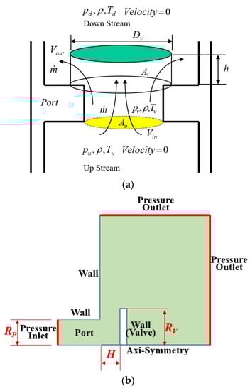
Figure 1.
Analysis model and boundary conditions. (a) Schematic of refrigerant flow near valve; (b) Analysis domain and boundary conditions.
- Valve is regarded as a circular plate. With this assumption, analysis is carried out in a 2D axi-symmetric plane;
- Flow is isentropic and steady;
- The upstream condition is stagnant;
- The open valve can be treated instantaneously as a simple orifice;
- The refrigerant is an incompressible ideal gas.
During the suction process, the pressure drop inside the cylinder is typically less than 30 kPa [16], but this can vary depending on the suction pressure and rotation speed. When the pressure difference is 30 kPa, the average velocity at the port is less than 100 m/s and the Mach number is less than 0.3, which allows us to assume an incompressible flow. However, it is important to note that this study’s results are limited to modeling the suction process, and further study on compressible flow is necessary to apply these findings to the discharge process, where the pressure difference exceeds 30 kPa.
The valve is regarded as rigid and treated as a wall in this analysis. The valve plate is also treated as a wall. No slip condition was imposed on the wall boundary. Pressure inlet and pressure outlet boundary conditions were imposed on the port and chamber boundary, respectively.
Based on the assumptions in Section 2.1 and the thermodynamic properties at the inlet and outlet, the actual mass flow rate can be calculated by [8,19,20]
where is the mass flow rate, K is the flow coefficient, A is the flow area, is the effective flow area, is the density of the refrigerant, and is the pressure difference between downstream and upstream. The flow from downstream to upstream is composed of two region, i.e., downstream to valve face and from valve face to upstream. The effective flow area from downstream to upstream can be expressed using each flow coefficient and the flow area of the two regions as [8,19,20]
where K0 and K1 are the flow coefficient of the port and valve open region, respectively. A0 and A1 are the cross-sectional area of the port and valve open region, respectively. The port area is simply calculated by . In contrast to the port area, the cross-sectional area of the valve open region is ambiguous. The cross-sectional area of the valve open region can be calculated by [8,19]
where R is the representative radius of the valve open region and H is the valve lift. There can be three options for choosing the representative radii, i.e., inner, outer, and average. In order to determine the representative radii, CFD analyses were conducted by varying the valve radius. The results of these analyses are presented in Figure 2, which shows that the mass flow rate is strongly influenced by the port area, but not by the valve radius. Therefore, the cross-sectional area of the valve open region is defined based on the port radii as
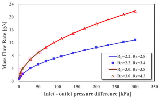
Figure 2.
Mass flow rate for various port and valve radius.
The effective force area can also be expressed as [19]
where is the effective force area, is the upstream pressure, and is the downstream pressure. When the port radius is constant, the effective force area can be expressed as [12,19]
In Equation (6), the effective force area continuously increases from 1.0 and saturates at a certain value as A1 increases. However, it was shown that the effective force area may decrease and can be smaller than 1.0 when the valve lift is small, as shown in Figure 3a [3,7]. The pressure force has a great effect on the valve dynamic behavior; therefore, its values have to be defined accurately. In this study, in order to define the pressure force on the valve surface, CFD analyses were carried out for various dimensions of the port, valve, and pressure differences. Based on the CFD analysis results, the effective force areas were defined.
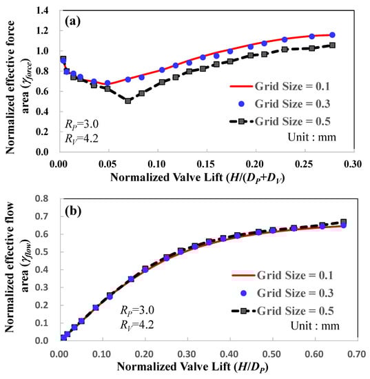
Figure 3.
Normalized (a) effective force area; and (b) effective flow area for three cases of grid size.
2.2. Grid Independency and Validation
Analyses were carried out for three grid sizes to confirm the grid independency. In these analyses, the port and valve radii are 3.0 and 4.2 mm, respectively. The analysis results are shown in Figure 3. When the grid size is smaller than or equal to 0.3 mm, the effective force areas are almost identical. The effect of grid size on the mass flow rate is not significant for the three cases of grid size. Based on these results, the grid size is set at 0.2 mm for all analyses in this study. The total number of nodes and grids varies depending on the analysis case, ranging from 4030 to 6235 nodes and 3866 to 5903 grids.
To validate the current analysis model, an analysis was carried out for the experiment of Gasche et al. [21]. The analysis model and conditions were the same as those in the experiment, with a port diameter of 34.90 mm, a circular plate diameter of 52.35 mm, a distance of 3.14 mm between the plate and port, and an inlet velocity of 1.2256 m/s. As shown in Figure 4, the pressure distribution along the radial direction was compared, and it was found that the analysis results obtained in the current study coincide well with the experimental results.
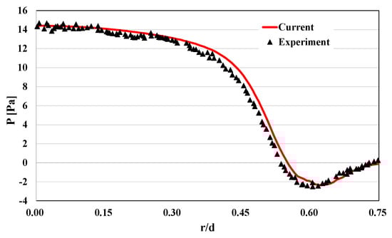
Figure 4.
Comparison of the pressure distribution along the radial direction obtained by experiment and CFD analysis.
3. Determination of Effective Flow and Force Areas
3.1. Effective Flow Area
The CFD analyses were carried out for various parameters such as pressure difference, valve lift, and valve and port radius. The analysis cases are shown in Table 1. In total, 380 analyses were carried out and all of these analysis results were used to obtain the model coefficients. R600a is used as a refrigerant, and its density is 2.51 kg/m³ at a temperature of 300 K and a pressure of 1.0 bar. Figure 5 shows the pressure and velocity distributions for the two cases of valve lift. When the valve lift was 0.5 mm, the pressures in the cylinder were almost identical and the pressure sharply dropped near the port end. When the valve lift was 2.0 mm, a velocity gradient existed inside the cylinder due to the high mass flow rate. The maximum velocity values were almost identical for the two cases of valve lift. When the valve lift was 0.5 mm, the maximum velocity was observed near the port end. This may cause low static pressure on the valve face; finally, negative pressure force may be induced. When the valve lift was 2.0 mm, maximum pressure was observed at the end of the valve. Therefore, lower negative pressure force was expected than in the case of valve lift of 0.5 mm.

Table 1.
Analysis cases (380 cases) (pout = 100.0 kPa).
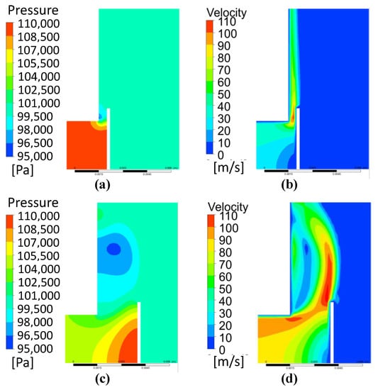
Figure 5.
Pressure and velocity distributions (pin =110 kPa, pout = 100 kPa, RP = 3.0 mm, RV = 3.8 mm): (a,b) valve lift = 0.5 mm; (c,d) valve lift =2.0 mm.
Mass flow rates were obtained through CFD analysis, and effective flow areas were then calculated using Equation (1). The effective flow area values obtained from the CFD analysis are shown by symbols in Figure 6, and were fitted to Equation (2). The fitting was performed using the ‘Solver’ function in Excel, with the coefficients K0 and K1 set as design variables. The error was defined as the sum of the differences between the predicted (fitted) and simulated effective flow areas. By minimizing this error, the coefficients K0 and K1 were found to be 0.707 and 0.586, respectively. A detailed explanation of the procedure used to determine these coefficients is provided in Section 3.2. The average fitting error was approximately 1.90%, indicating that Equation (2) accurately describes the effective flow area.
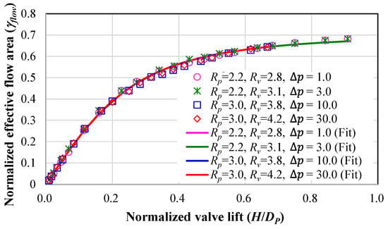
Figure 6.
Normalized effective flow area for various geometries and pressure differences, and fitted results.
3.2. Effective Force Area
The effective force area values were also calculated by Equation (5) using the CFD analysis results for various pressure differences and valve and port radii. Figure 7 shows the normalized effective force area for the valve lift. In all cases of port and valve radii, decreasing and increasing zones were observed. To confirm the decreasing phenomena of the effective force area, the pressure distributions according to the valve positions for the three cases of valve lift are shown in Figure 8. When the valve lifts were 0.1 and 0.3 mm, the pressure on the bottom face became lower than the pressure on the top face. When the valve lift is 0.3 mm, the pressure is lower than the pressure of the 0.1 mm valve lift. This explain the decrease in pressure force in Zone 1 (‘Z1’, in Figure 7).
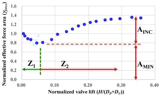
Figure 7.
Normalized effective force area for various values of valve lift (RP = 2.2 mm, RV = 3.4 mm, and = 1.0 kPa).
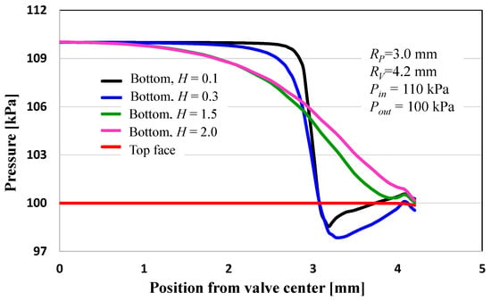
Figure 8.
Pressure distributions on top and bottom faces of valve for three cases of valve lift.
Considering the effective force area shown in Figure 7, the effective force area model was proposed as
where and are the effective force area models obtained using decreasing and increasing zone data, respectively. For example, when the normalized valve lift is 0.02, as shown in Figure 7, is higher than ; then, is selected for the effective force area. When the normalized valve lift is 0.2, is higher than ; then, is selected for the effective force area.
The decreasing slope and amount are dependent on the port and the valve radius. The effective force area is expected to be saturated at a certain value, and then decrease. In this study, the valve lift was assumed to be smaller than the lift at which the effective force area was saturated. Therefore, the decrease of the effective force area after saturation was not considered. The saturated effective force area was also dependent on the port and valve radius. Figure 9 shows the minimum and the maximum effective force area values for the given ratio of valve area to port area. It can be seen that the maximum effective force area increased linearly with the area ratio, and the minimum effective force area decreased linearly with the area ratio. These linear relationships of the maximum and minimum effective force area are only reliable for the port and valve geometries and pressure values used in this study. The authors found that a decrease in effective force area in ‘Z1’, shown in Figure 7, can be described well by an exponential function. Therefore, the normalized effective force area of ‘Z1’ is proposed as
where a1 to a5 are the coefficients that should be determined. The first and second terms in Equation (8) stand for the minimum and the decrease of the effective force area, respectively.
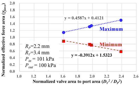
Figure 9.
Normalized effective force area for ratio of valve to port area (RP = 2.2, RV = 3.4 mm, = 1.0 kPa).
The authors found that the effective force area in ‘Z2’, shown in Figure 7, can be described by the logarithmic function
where C, D, b1, and b2 are the coefficients that should be determined. The coefficients C and D control the slope increase and offset of the effective force area. The second set of coefficients controls the maximum increase in the effective force area. The coefficients C and D are dependent on the pressure differences. Figure 10 shows the pressure dependency of coefficients C and D. The coefficients C and D slightly decrease linearly as the pressure difference increases. Therefore, the coefficients C and D were modeled as
where g1 to g4 are the model coefficients that should be determined.
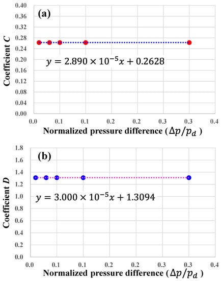
Figure 10.
Pressure dependency of coefficients C and D (RP = 2.2, RV = 3.4 mm).
The coefficients a1, a2, a3, a4, a5, b1, b2, g1, g2, g3, and g4 were determined by optimization using the Excel solver function. The optimization problem was defined as
Minimize Error (a1, a2, a3, a4, a5, b1, b2, g1, g2, g3, g4, pin, pout, H, DP, DV)
Design variable: a1, a2, a3, a4, a5, b1, b2, g1, g2, g3, g4
In Equation (11a), Error was defined as the sum of the fitting error as
where n is the number of simulation cases, as shown in Table 1 (n = 380); and are the effective force areas obtained by simulation and fitting, respectively. pin, pout, H, DP, and DV are the CFD analysis conditions.
By the optimization of Equation (11) using the 380 analysis results, the coefficients of the effective force area model were determined. The determined coefficients are shown in Table 2.
Table 2.
Determined coefficients of effective force area model.
The effective force area, obtained by the CFD analysis, and the effective force area, calculated using Equations (7)–(10) with the coefficients given in Table 2, are compared in Figure 11. The outlet pressure, pout, is fixed to 100 kPa in the analysis. Figure 11a,b shows the results for inlet pressure (pin) of 101 kPa. Figure 11c–d and Figure 11e,f show the results for inlet pressures of 200 and 300 kPa, respectively. Figure 11a,c,d shows results for port radii of 2.2 mm. Additionally, Figure 11b–f shows results for port radii of 3.0 mm. The minimum effective force area, the decrease and increase in the effective force area as the valve lift increases, and the decreasing slope are predicted well by the proposed effective force area model of Equations (7)–(10). It can be seen that the decrease in the normalized effective force area decreases more and faster as the valve diameter increases. Additionally, the maximum normalized effective force area increases as the valve diameter increases. The normalized valve lift, at which the effective force area is at its minimum, is highly dependent on the ratio of valve diameter to port diameter. The average fitting error of 380 analysis cases was 2.9%. As a result, the effective force area can be accurately calculated by the proposed model of Equations (7)–(10) in a wide range of pressure differences up to 200 kPa, and can be used in the dynamic analysis of the valve. In the model, a quadratic dependency of the effective force area on the valve-to-port diameter was assumed; therefore, the proposed model is valid only for port diameters from 2.2 to 3.0 mm, and valve-to-port diameters from 1.26 to 1.55. Additionally, the normalized valve lift, H/(DP + DV), is valid only up to about 0.4.
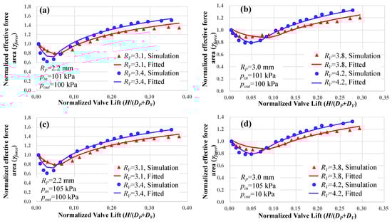
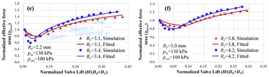
Figure 11.
Comparison of normalized effective force area obtained by CFD analysis and fitting: (a) RP = 2.2 mm, pin = 101 kPa; (b) RP = 3.0 mm, pin = 101 kPa; (c) RP = 2.2 mm, pin = 105 kPa; (d) RP = 3.0 mm, pin = 105 kPa; (e) RP = 2.2 mm, pin = 130 kPa; and (f) RP = 3.0 mm, pin = 130 kPa.
4. Conclusions
Based on the CFD analysis results, models were developed for the effective flow and force areas. The CFD analysis was performed for various values of pressure difference, valve and port diameter, and valve lift, and the effective flow and force areas were extracted for each case. The relationship between the effective flow area and pressure difference, valve lift, and port and valve diameters was investigated, leading to the proposal of a new effective force area model. Based on this study, the following conclusions were drawn:
- The effective flow area is highly dependent on the port diameter, but not on the valve diameter. Therefore, the side area of the open valve is defined using valve port area as ;
- The coefficients of effective flow area were determined to minimize the fitting error by the optimization of the Excel software. The average fitting error was smaller than 10−5. This means that the fitting with these coefficients was very accurate;
- The effective force area was very complex and highly dependent on valve lift and on the ratio of valve diameter to port diameter. When the normalized valve lift was small, the effective force area decreased as the valve lift increased. The minimum effective force area was found to be dependent on the ratio of the valve diameter to port diameter;
- The normalized effective force area model was proposed based on the CFD analysis results for various values of pressure difference, valve lift, and port and valve diameters. The decrease and increase in the effective force area were modeled by exponential and logarithmic functions, respectively. The minimum and maximum effective force area values were modeled by a linear function of the ratio of the valve area to port area;
- The model coefficients of the normalized effective force area were determined by minimizing the fitting error. The average error was 2.9%.
As a result, the effective flow and force area model proposed in this study can accurate describe the mass flow rate and pressure force on the valve face. The implementation of this model in the performance analysis of a compressor or the dynamic analysis of a reed valve will be carried out in a separate study.
Author Contributions
Conceptualization, J.B.K.; methodology, J.B.K.; validation, S.J.L.; formal analysis, J.D.P.; resources, J.K.; data curation, J.-y.A.; writing—original draft, J.B.K. All authors have read and agreed to the published version of the manuscript.
Funding
This study was supported by the research program funded by the SeoulTech (Seoul National University of Science and Technology).
Data Availability Statement
Not applicable.
Conflicts of Interest
The authors declare no conflict of interest.
Abbreviations
| SI Unit Nomenclature | |
| Port area [ ]. | |
| Cylindrical face area between valve and plate () [ ]. | |
| Effective flow area. | |
| Effective force area [ ]. | |
| Port diameter [mm]. | |
| Valve diameter [mm]. | |
| F | Force acting on reed valve [N]. |
| H | Valve lift [m]. |
| Mass flow rate through the port [Kg/s]. | |
| Inlet pressure [Pa]. | |
| Outlet pressure [Pa]. | |
| Upstream pressure [Pa]. | |
| Downstream pressure [Pa]. | |
| Pressure difference between and [Pa]. | |
| Port radius [mm]. | |
| Valve radius [mm]. | |
| Density of refrigerant [Kg/ ]. | |
| Dimensionless Number Nomenclature | |
| Normalized effective flow area (). | |
| Normalized effective force area (). | |
| Normalized effective force area of decreasing region (). | |
| Normalized effective force area of increasing region () Normalized valve lift (). | |
| Coefficient Nomenclature | |
| K | Flow coefficient. |
| Flow coefficient at port. | |
| Flow coefficient between port and valve. | |
| Force coefficient for decreasing region. | |
| Force coefficient for increasing region related to port to valve diameter. | |
| Force coefficient for increasing region related to pressure and valve lift. | |
References
- Soedel, W. Design and Mechanics of Compressor Valves; Purdue University: West Lafayette, IN, USA, 1984. [Google Scholar]
- Kim, M.H.; Bullard, C.W. Thermal Performance Analysis of Small Hermetic Refrigeration and Air-Conditioning Compressors. JSME Int. J. 2002, 45, 857–864. [Google Scholar] [CrossRef]
- Ferreira, T.S.; Lainor, J. Analysis of the Influence of Valve Geometric Parameters on the Effective Flow and Force Areas. In Proceedings of the International Compressor Engineering Conference, West Lafayette, IN, USA, 4–7 August 1986; pp. 558–646. [Google Scholar]
- Dabri, A.E.; Rice, C.K. A Compressor Simulation Model with Corrections for the Level of Suction Gas Superheat. ASHRAE Trans. 1981, 87, 771–782. [Google Scholar]
- Prakash, R.; Singh, R. Mathematical Modeling and Simulation of Refrigerating Compressors. In Proceedings of the International Compressor Engineering Conference, West Lafayette, IN, USA, 10–12 July 1974; pp. 274–285. [Google Scholar]
- Tan, Q.; Liu, Z.; Cheng, J.; Feng, Q. Effective Flow and Force Areas of Discharge Valve in A Rotary Compressor. In Proceedings of the International Compressor Engineering Conference, West Lafayette, IN, USA, 14–17 July 2014. [Google Scholar]
- Ferreira, R.l.; Gasche, J.L. Effective force area and discharge coefficient for reed type valves: A comprehensive data set from a numerical study. Int. J. Refrig. 2019, 103, 287–300. [Google Scholar] [CrossRef]
- Kerpicci, H.; Oguz, E. Transient Modeling of Flows Through Suction Port and Valve Leaves of Hermetic Reciprocating Compressors. In Proceedings of the International Compressor Engineering Conference, West Lafayette, IN, USA, 17–20 July 2006; Available online: https://docs.lib.purdue.edu/icec/1806 (accessed on 2 September 2021).
- Dhar, S.; Ding, H.; Lacerda, J. A 3-D Transient CFD Model of a Reciprocating Piston Compressor with Dynamic Port Flip Valves. In Proceedings of the International Compressor Engineering Conference, West Lafayette, IN, USA, 11–14 July 2016; Available online: https://docs.lib.purdue.edu/icec/2471 (accessed on 3 October 2021).
- Wu, W.; Guo, T.; Peng, C.; Li, X.; Li, X.; Zhang, Z.; Xu, L.; He, Z. FSI simulation of the suction valve on the piston for reciprocating compressors. Int. J. Refrig. 2022, 137, 14–21. [Google Scholar] [CrossRef]
- Wang, Y.; Wang, J.; He, Z.; Sun, J.; Wang, T.; Liu, C. Investigation on Dynamic Characteristics of the Reed Valve in Compressors Based on Fluid-Structure Interaction Method. Appl. Sci. 2021, 11, 3946. [Google Scholar] [CrossRef]
- An, K.H.; Lee, J.H.; Lee, I.W.; Lee, I.S.; Park, S.C. Performance Prediction of Reciprocating Compressor. In Proceedings of the International Compressor Engineering Conference, West Lafayette, IN, USA, 16–19 July 2002; Available online: https://docs.lib.purdue.edu/icec/1525 (accessed on 15 January 2022).
- Achour, M.; Boumediene, T.; Brahaim, D. Unsteady state numerical simulation of reciprocating compressor in the presence of the suction and discharge process. U. P. B. Sci. Bull. 2020, 82, 161–178. [Google Scholar]
- Wang, Y.; Jiang, Z.; Zhang, J.; Zhou, C.; Liu, W. Performance analysis and optimization of reciprocating compressor with stepless capacity control system under variable load conditions. Int. J. Refrig. 2018, 94, 174–185. [Google Scholar] [CrossRef]
- Liu, Z.; Cao, X.; Wang, T.; Jia, W.; Duan, Z. Comparative evaluation of the refrigeration compressor performance under different valve parameters in a trans-critical CO2 cycle. Int. J. Refrig. 2019, 101, 34–46. [Google Scholar] [CrossRef]
- Diniz, M.C.; Hermes, C.J.L.; Deschamps, C.J. Transient simulation of small-capacity reciprocating compressors in on-off controlled refrigerators. Int. J. Refrig. 2019, 102, 12–21. [Google Scholar] [CrossRef]
- Guo, J.; Li, B.; Wang, S.; Hu, W.; He, Z. Calculation of Flow Coefficient and Effective Action Area Coefficient of Compressor’s Reed Valve based on Fluid—Solid Coupling. In Proceedings of the International Conference on Aircraft Utility Systems (AUS), Beijing, China, 10–12 October 2016. [Google Scholar]
- Wei, Z.; Ziwen, X.; Xueyuan, P. Investigation on the Suction Reed Valve Motion with Sticky Force in a Refrigerator Compressor. Energies 2018, 11, 2897. [Google Scholar] [CrossRef]
- Schwerzler, D.D.; Hamilton, J.F. An Analytical Method for Determining Effective Flow and Force Areas for Refrigeration Compressor Valving Systems. In Proceedings of the International Compressor Engineering Conference, West Lafayette, IN, USA, 25–27 July 1972; pp. 30–36. [Google Scholar]
- Soedel, W. Sound and Vibrations of Positive Displacement Compressors; CRC Press: Boca Raton, FL, USA, 2007; ISBN 978-0849370496. [Google Scholar]
- Gasche, J.L.; Arantes, D.M.; Andreotti, T. Pressure distribution on the frontal disk for turbulant flows in a radial diffuser. Exp. Therm. Fluid Sci. 2015, 60, 317–327. [Google Scholar] [CrossRef]


Disclaimer/Publisher’s Note: The statements, opinions and data contained in all publications are solely those of the individual author(s) and contributor(s) and not of MDPI and/or the editor(s). MDPI and/or the editor(s) disclaim responsibility for any injury to people or property resulting from any ideas, methods, instructions or products referred to in the content. |
© 2023 by the authors. Licensee MDPI, Basel, Switzerland. This article is an open access article distributed under the terms and conditions of the Creative Commons Attribution (CC BY) license (https://creativecommons.org/licenses/by/4.0/).