
Rate Decline of Acid Fracturing Stimulated Well in Bi-Zone Composite Carbonate Gas Reservoirs
Abstract
:1. Introduction
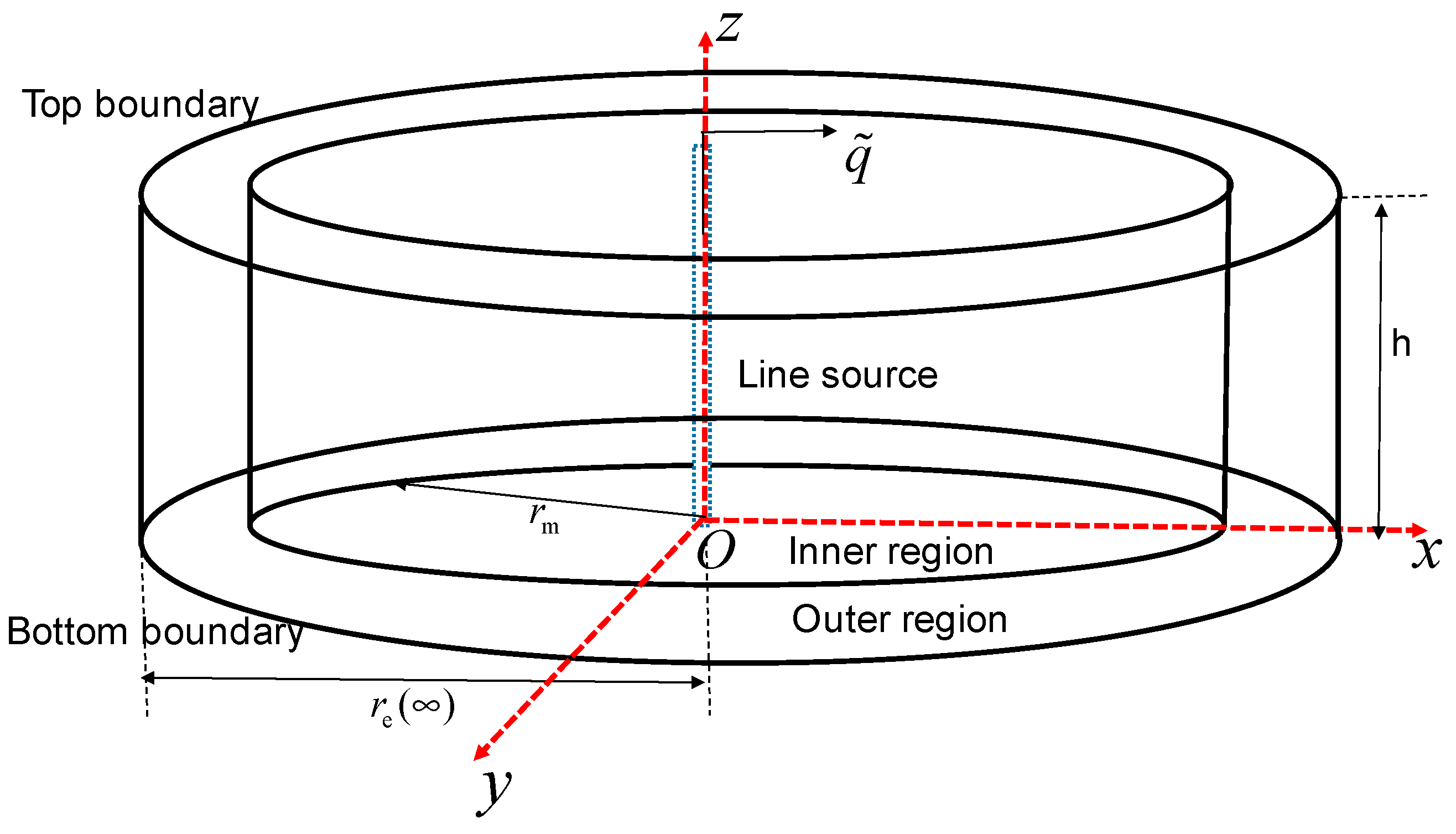
2. Physical Model
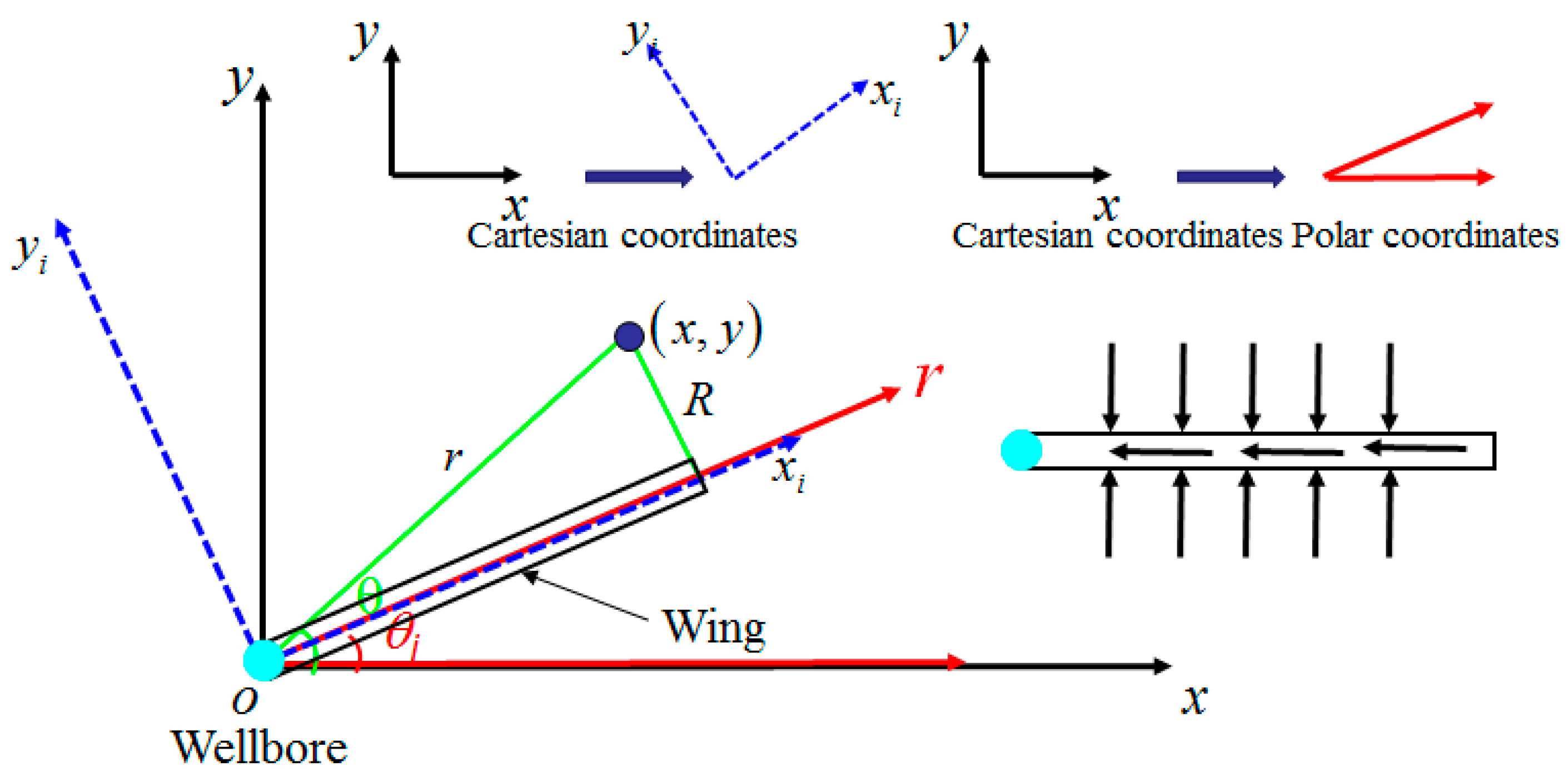
- The length of each hydraulic fracture is not equal, considering existence of angle (θ) between fracture and horizontal direction. The length (Lf), width (Wf), and permeability (kf) of the different hydraulic fractures are different;
- The fluid in the reservoir conforms to Darcy’s law and law of isothermal percolation;
- The upper and bottom boundaries of the reservoir are closed, and the fluid is incompressible;
- Stress sensitivity of permeability in tight reservoirs is taken into account;
- Negligible gravity and capillary effect are studied.
3. Mathematical Model
3.1. Line-Source Model in Bi-Zone Composite Reservoirs Considering Stress Sensitivity
- (1)
- Governing differential equation of inner region can be written as
- (2)
- Governing differential equation of outer region can be written as
- (3)
- Inner boundary condition can be written as
- (4)
- Infinite lateral boundary condition can be written as
- (5)
- Interface condition between the inner and the outer region can be written as
3.2. Surface-Source Model in Bi-Zone Composite Reservoirs Considering Stress Sensitivity
3.3. Coupling of Reservoir Model and Hydraulic Fracture Model
4. Mathematical Model Solution
5. Results and Discussion
6. Conclusions
- (1)
- Complicated fractures around the wellbore during refracturing measurement can be modeled using a modified multiple fractures model. Based on the theory of point function, when stress sensitivity is considered, the result of the multiple fractures model describing complicated fractures can be solved analytically in the Laplace domain.
- (2)
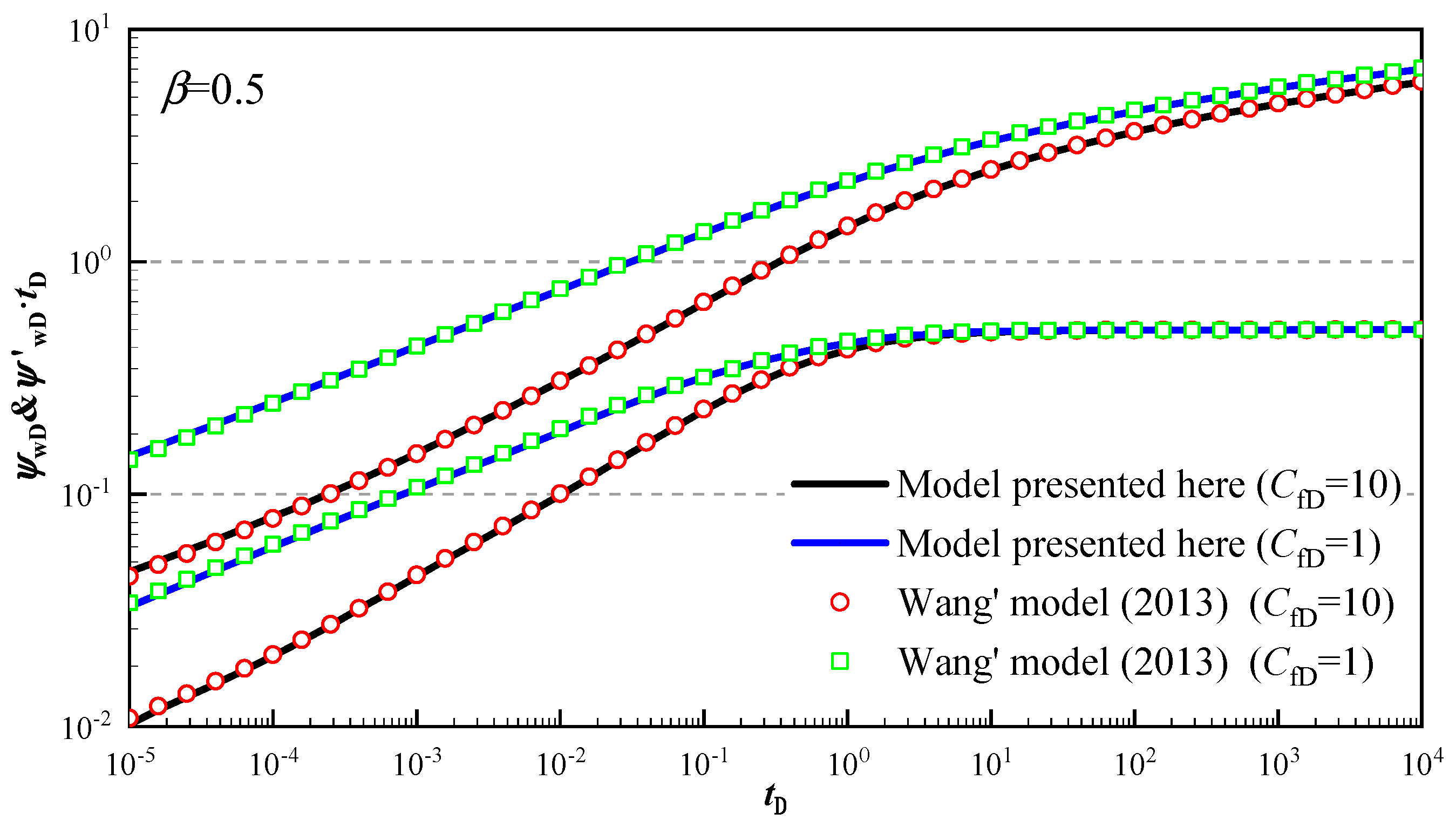
- We compared the simplified model obtained from this paper with the result calculated by Wang for asymmetry fracture without stress sensitivity and the result calculated by the commercial well-test simulator for symmetric fracture of bi-zonal composite reservoirs without stress sensitivity, respectively. The results showed excellent agreement.
- (3)
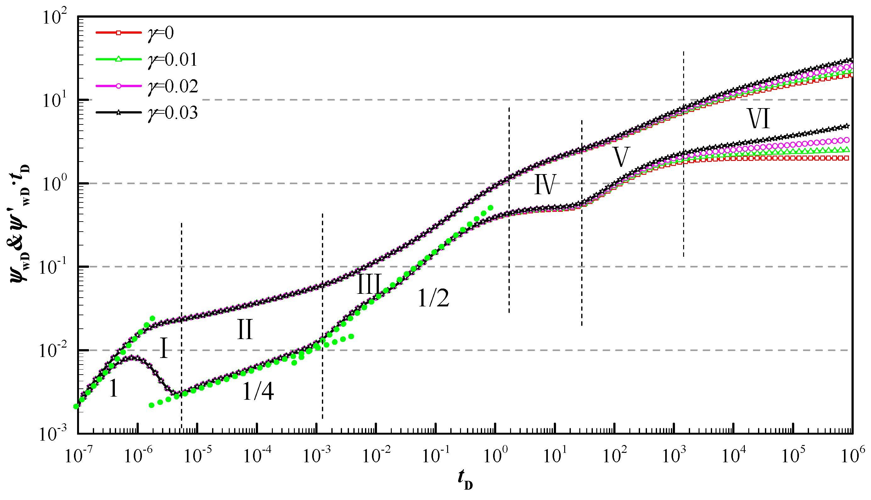
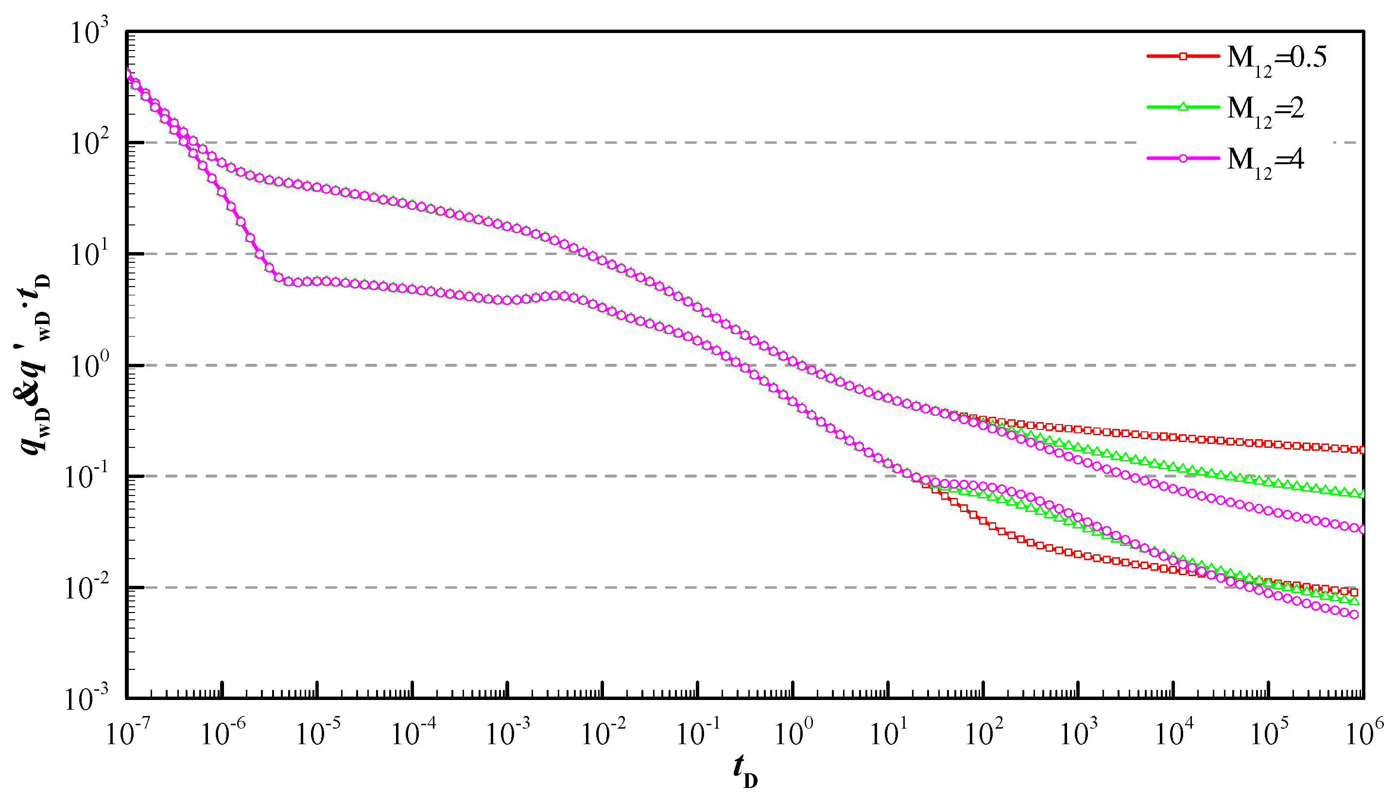
- The log–log typical curves can be generated using a solution of this model, which mainly includes the bi-linear flow stage (quarter-slope portion), followed by the linear flow stage (quarter-slope portion), then the radial flow stage of the stimulated region (0.5 value) and radial flow stage of the un-stimulated region (0.5 M12 value, without stress sensitivity).
- (4)
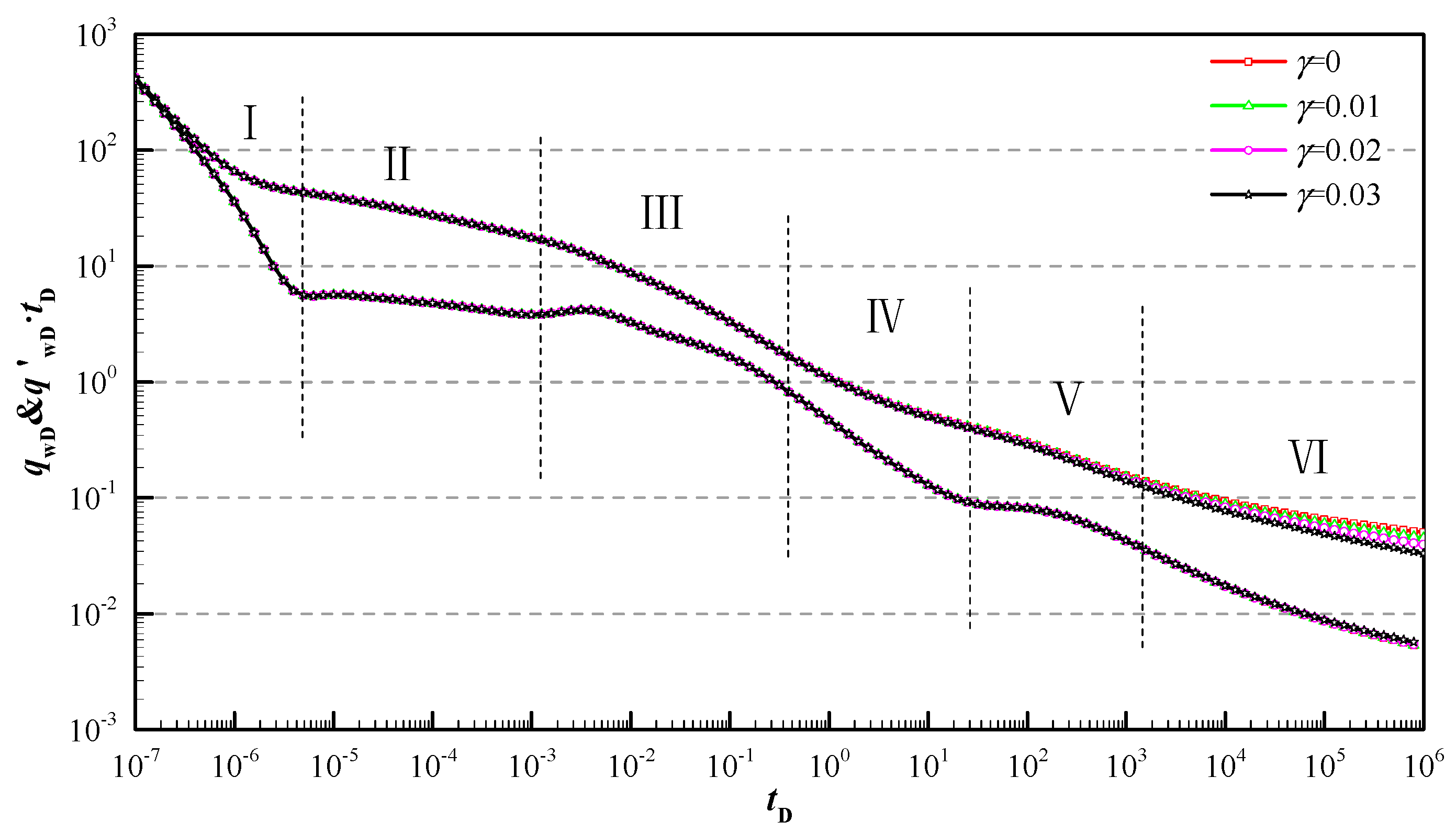
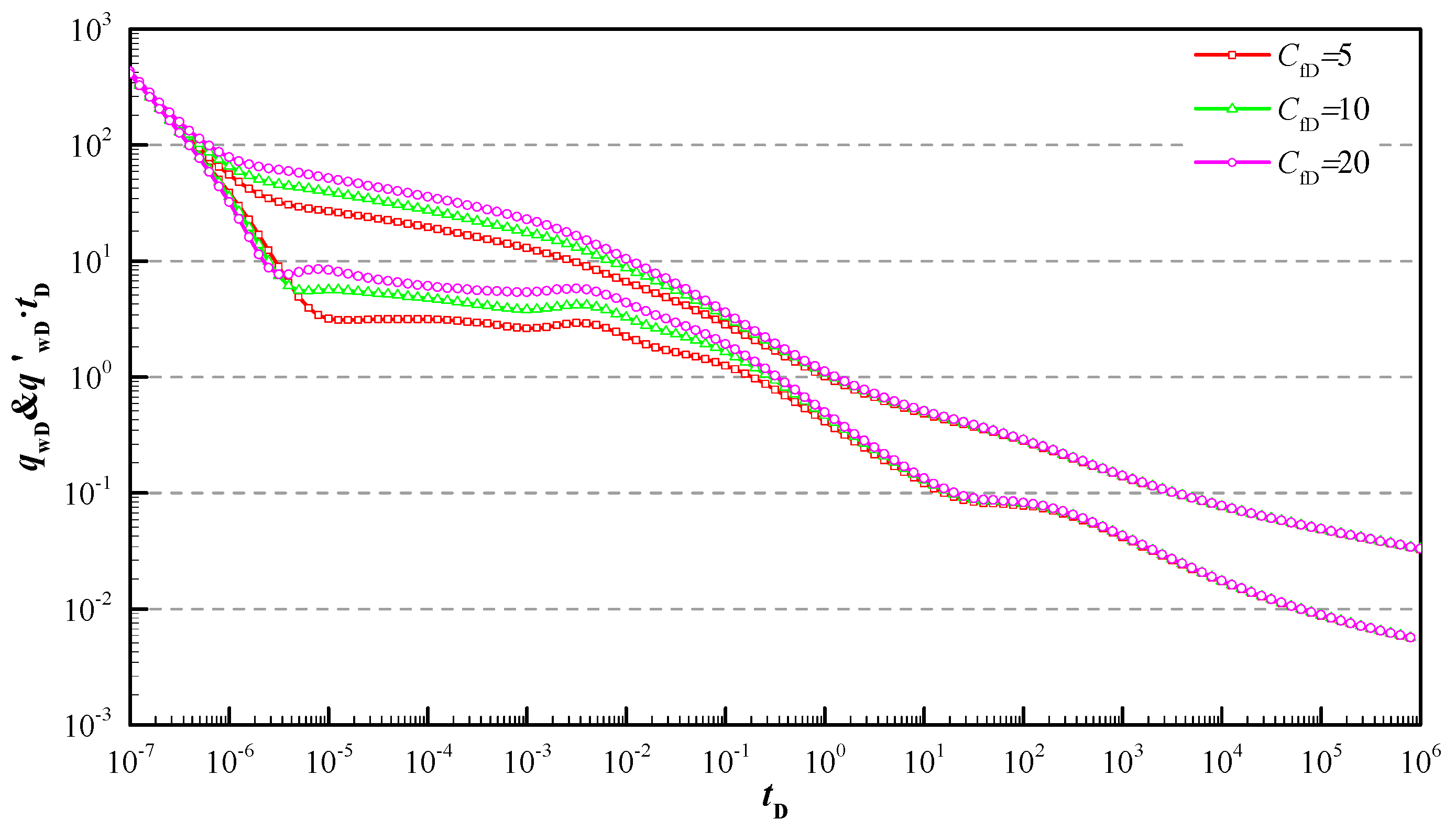
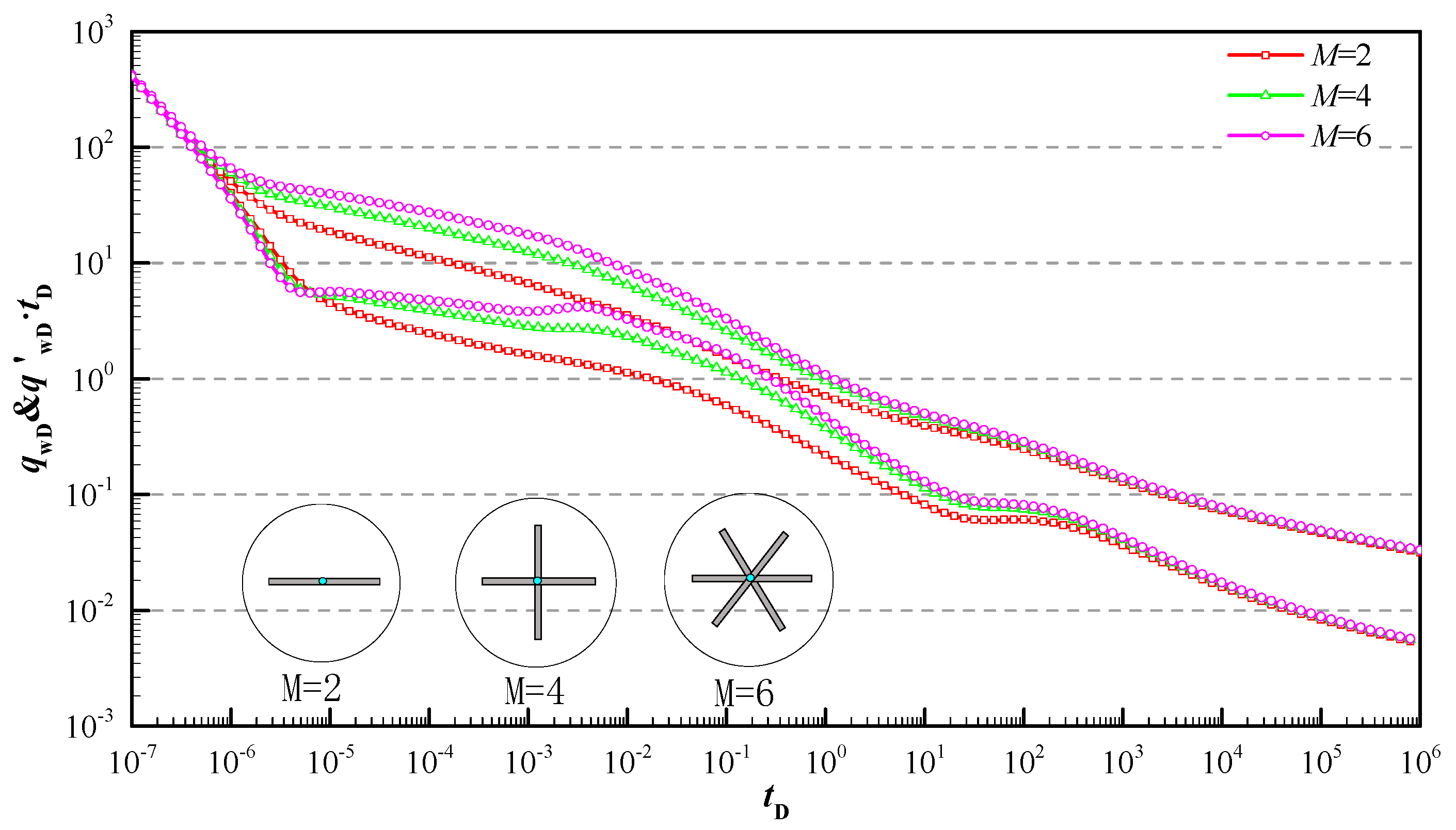
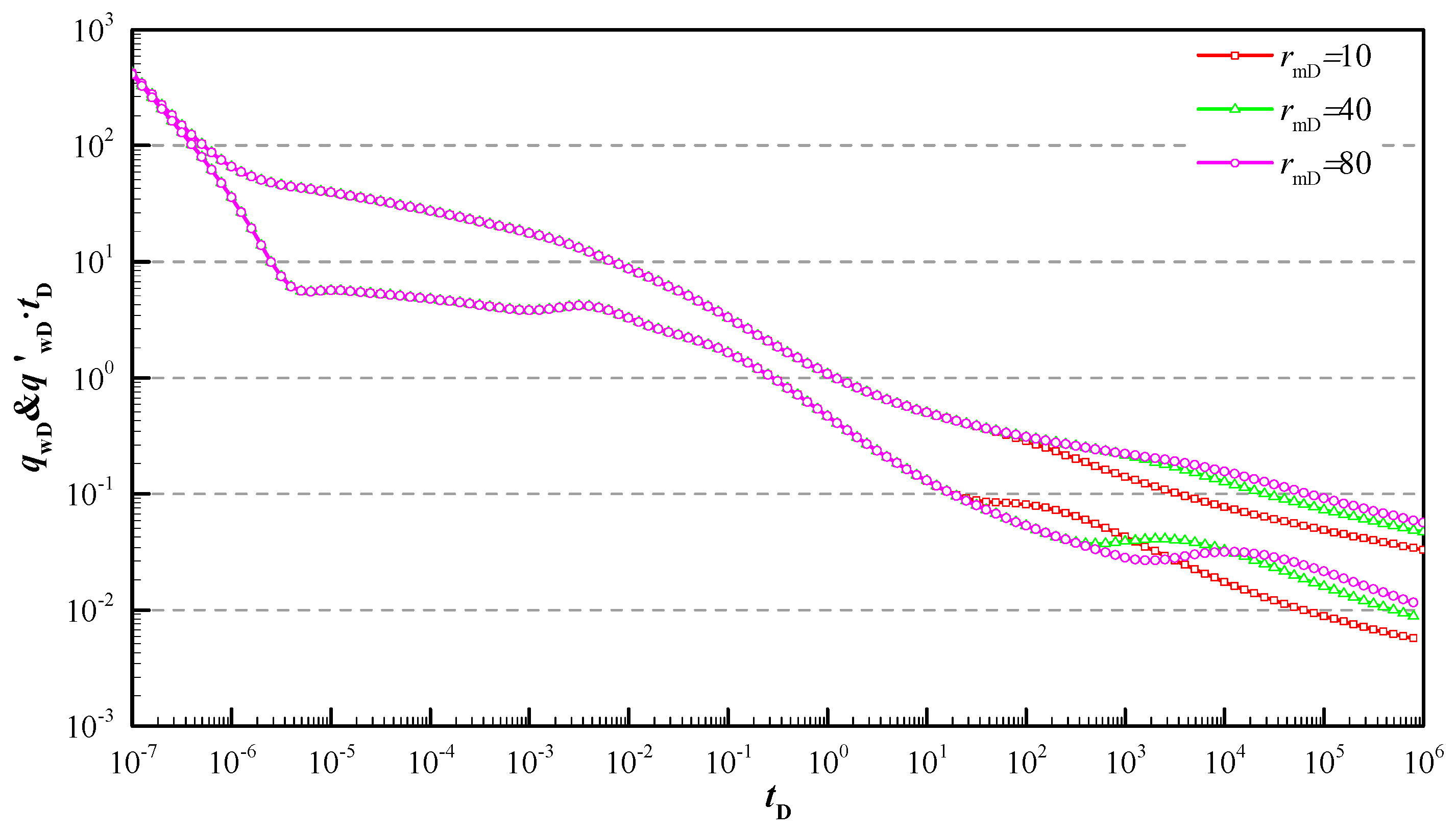
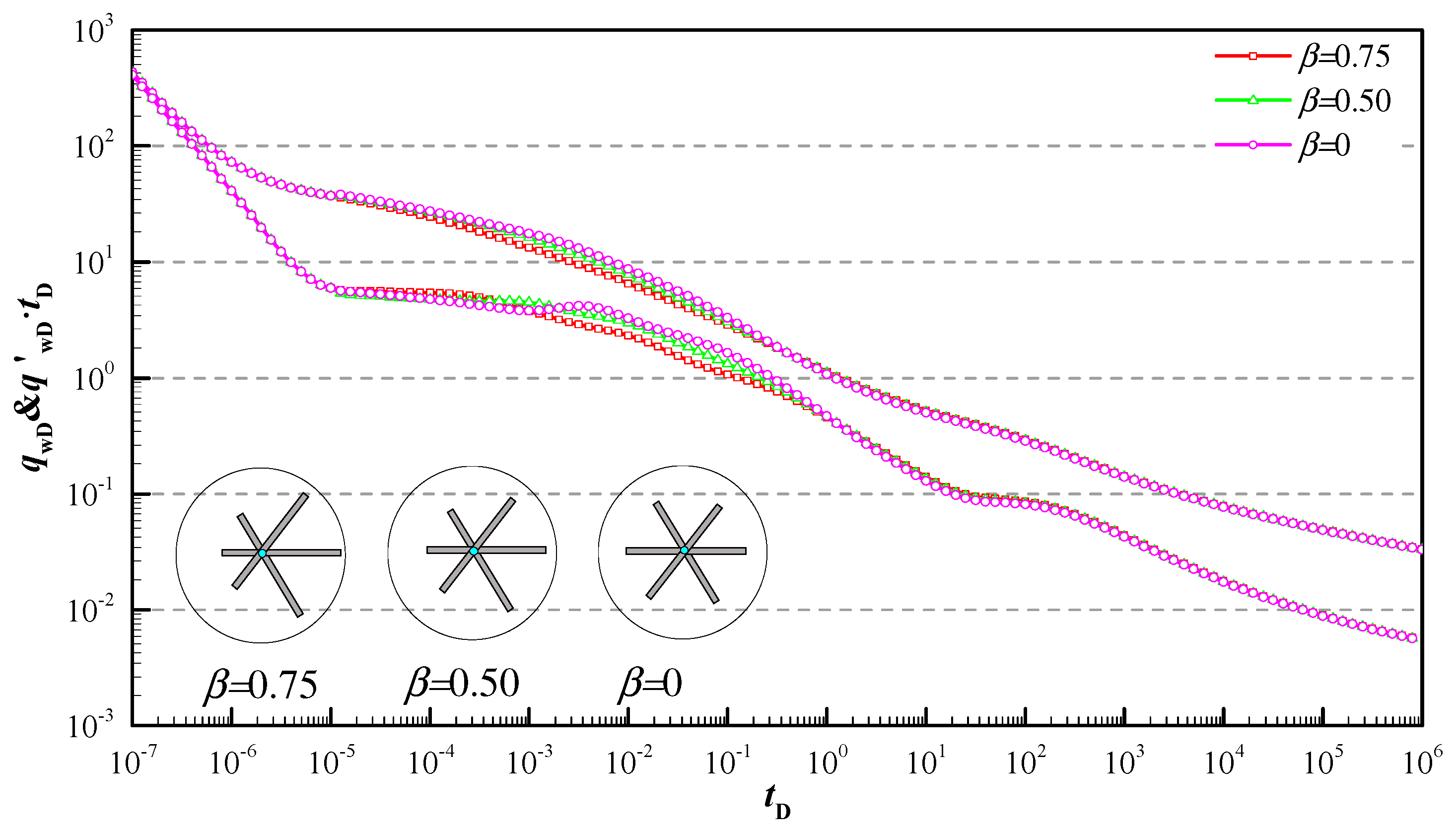
- The model illustrated how the transient production rate curves are influenced by reservoir and hydraulic fracture parameters. Reasonable fracture distribution can effectively decrease the pseudo-pressure loss of the early stage, and the more uneven the fracture distribution along the angle is, the lower the pseudo-pressure curve is; the smaller asymmetric factor leads to larger pseudo-pressure loss and the unobvious bi-linear characteristic.
Author Contributions
Funding
Institutional Review Board Statement
Informed Consent Statement
Data Availability Statement
Conflicts of Interest
Nomenclature
| Wellbore storage coefficient, Pa/m3 | |
| Skin factor, dimensionless | |
| Production time, s | |
| Hydraulic fracture permeability, m2 | |
| Permeability of inner region, m2 | |
| Permeability of outer region, m2 | |
| Original reservoir permeability, m2 | |
| permeability modulus, Pa−1 | |
| Width of hydraulic fracture, m | |
| Original reservoir pseudo-pressure, Pa | |
| Pseudo-pressure of inner region, Pa | |
| Wellbore pseudo-pressure, Pa | |
| Pseudo-pressure of un-stimulated region, Pa | |
| Pseudo-pressure of hydraulic fracture, Pa | |
| Gas viscosity, Pa.s | |
| Total compressibility, Pa−1 | |
| Tiny variable, dimensionless | |
| Zero-order perturbation deformation function | |
| Reservoir porosity, dimensionless | |
| Reference length, m; | |
| Length of wing, m | |
| Zero-order perturbation deformation function of inner region | |
| Zero-order perturbation deformation function of hydraulic fracture | |
| Angle between the fracture and the horizontal axis, degree | |
| Radius of inner region, m | |
| Directional coordinates, m | |
| Zero-order perturbation deformation function of inner region | |
| Zero-order perturbation deformation function of hydraulic fracture | |
| Angle between the fracture and the horizontal axis, degree | |
| Radius of inner region, m | |
| x- and y-coordinates of line source, m | |
| Hydraulic fractures number, integer | |
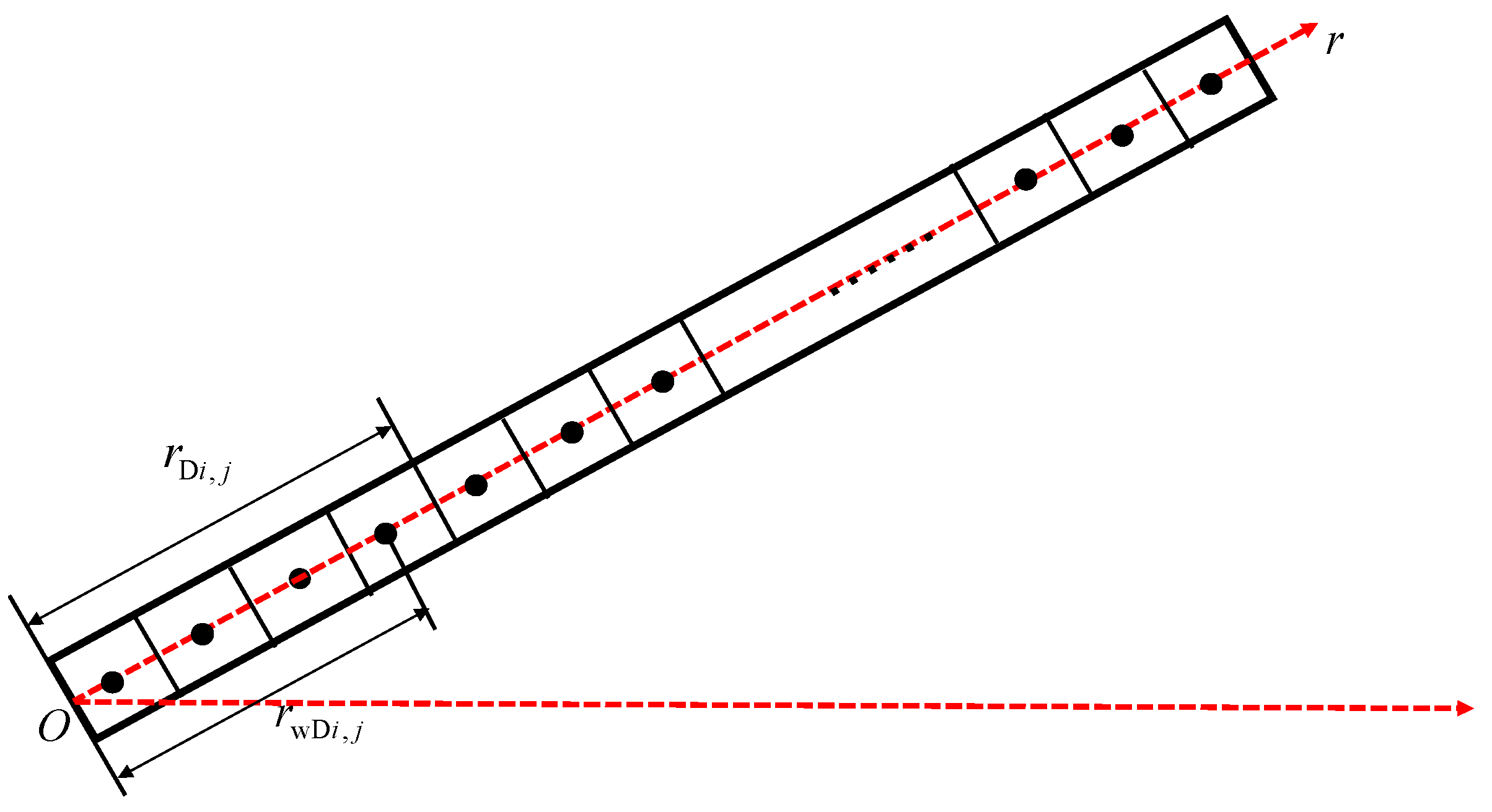
| Grid number of hydraulic fractures dispersed, integer | |
| Strength of continuous line source, m2/s | |
| Strength of continuous fracture line source, m2/s | |
| Production rate of hydraulic fractures, m3/s | |
| Production rate, m3/s | |
| Mobility ratio of inner and outer region, | |
| Diffusivity ratio of inner and outer region, fraction | |
| Asymmetry factor, dimensionless | |
| Grid spacing, | |
| Node i-th hydraulic fractures is the j-th grid | |
| Middle node i-th hydraulic fractures is the j-th grid | |
| The second kind modified Bessel function | |
| The first kind modified Bessel function | |
| Laplace variables | |
| Subscripts | |
| Dimensionless | |
| Inner region | |
| Outer region, | |
| Initial state | |
| ith hydraulic fractures | |
| jth grid | |
| Standard state | |
| Wellbore | |
| Hydraulic fractures | |
| Superscripts | |
| Variables in the Laplace domain | |
| ′ | Derivative |
Appendix A

| Variables | Dimensionless Definition | Variables | Dimensionless Definition |
|---|---|---|---|
| Dimensionless pseudo-pressure of inner region | Dimensionless z-coordinate | ||
| Dimensionless pseudo-pressure of outer region | Dimensionless radius of boundary | ||
| Dimensionless hydraulic fracture pseudo-pressure | Dimensionless hydraulic fracture conductivity | ||
| Dimensionless production time | Dimensionless length of wing | ||
| Dimensionless distance | Dimensionless continuous production | ||
| Dimensionless radius of inner region | Permeability ratio | ||
| Dimensionless x-coordinate | Diffusivity ratio | ||
| Dimensionless y-coordinate | Dimensionless stress-sensitivity coefficient |
References
- Urban, E.; Orozco, D.; Fragoso, A.; Selvan, K.; Aguilera, R. Refracturing vs. Infill drilling—A cost effective approach to enhancing recovery in shale reservoirs. Presented at the Unconventional Resources Technology Conference, San Antonio, TX, USA, 1–3 August 2016. URTEC-2461604-MS. [Google Scholar]
- Zhang, F.; Mack, M. Integrating fully coupled geomechanical modeling with microsesmicity for the analysis of refracturing treatment. J. Nat. Gas Sci. Eng. 2017, 46, 16–25. [Google Scholar] [CrossRef]
- Zhai, Z.; Sharma, M.M. Estimating fracture reorientation owing to long term fluid injection production. Presented at the Production and Operations Symposium, Oklahoma City, OK, USA, 31 March–3 April 2007. SPE-106387-MS. [Google Scholar]
- Wolhart, S.L.; McIntosh, G.E.; Zoll, M.B.; Weijers, L. Surface tiltmeter mapping shows hydraulic fracture reorientation in the Codell formation, Wattenberg field, Colorado. Presented at the SPE Annual Technical Conference and Exhibition, Anaheim, CA, USA, 11–14 November 2007. SPE-110034-MS. [Google Scholar]
- Fisher, M.; Wright, C.; Davidson, B.; Steinsberger, N.P.; Buckler, W.S.; Goodwin, A.; Fielder, E.O. Integrating Fracture Mapping Technologies To Improve Stimulations in the Barnett Shale. SPE Prod. Facil. 2005, 20, 85–93. [Google Scholar] [CrossRef]
- Cipolla, C.L.; Warpinski, N.R.; Mayerhofer, M.J.; Lolon, E.P.; Vincent, M.C. The relationship between fracture complexity, reservoir properties, and fracture treatment design. SPE Prod. Oper. 2008, 25, 438–452. [Google Scholar]
- Mittal, A.; Rai, C.S.; Sondergeld, C.H. Proppant-conductivity testing under simulated reservoir conditions: Impact of crushing, embedment, and diagenesis on long-term production in shales. SPE J. 2018, 23, 1304–1315. [Google Scholar] [CrossRef]
- Teng, B.; Andy Li, H. A semianalytical model for evaluating the performance of a refractured vertical well with an orthogonal refracture. SPE J. 2019, 24, 891–911. [Google Scholar] [CrossRef]
- Dejam, M.; Hassanzadeh, H.; Chen, Z. Semi-analytical solution for pressure transient analysis of a hydraulically fractured vertical well in a bounded dual-porosity reservoir. J. Hydrol. 2018, 565, 289–301. [Google Scholar] [CrossRef]
- Zhang, L.; Kou, Z.; Wang, H.; Zhao, Y.; Dejam, M.; Guo, J.; Du, J. Performance analysis for a model of a multi-wing hydraulically fractured vertical well in a coalbed methane gas reservoir. J. Pet. Sci. Eng. 2018, 166, 104–120. [Google Scholar] [CrossRef]
- Meng, M.; Chen, Z.; Liao, X.; Wang, J.; Shi, L. A well-testing method for parameter evaluation of multiple fractured horizontal wells with non-uniform fractures in shale oil reservoirs. Adv. Geo-Energy Res. 2020, 4, 187–198. [Google Scholar] [CrossRef]
- Xia, D.; Yang, Z.; Li, D.; Zhang, Y.; Zhao, X.; Yao, L. Research on numerical method for evaluation of vertical well volume fracturing effect based on production data and well test data. J. Pet. Explor. Prod. 2021, 11, 1855–1863. [Google Scholar] [CrossRef]
- Cui, Y.; Jiang, R.; Gao, Y.; Lin, J. Semi-analytical modeling of rate transient for a multi-wing fractured vertical well with partially propped fractures considering different stress-sensitive systems. J. Pet. Sci. Eng. 2022, 208, 109548. [Google Scholar] [CrossRef]
- Zhao, Y.L.; Zhang, L.H.; Liu, Y.H.; Hu, S.Y.; Liu, Q.G. Transient pressure analysis of fractured well in bi-zonal gas reservoirs. J. Hydrol. 2015, 524, 89–99. [Google Scholar] [CrossRef]
- Wang, L.; Wang, X. Type Curves Analysis for Asymmetrically Fractured Wells. J. Energy Resour. Technol. 2014, 136, 119–129. [Google Scholar] [CrossRef]
- Rodriguez, F.; Cinco-Ley, H. Evaluation of Fracture Asymmetry of Finite-Conductivity Fractured Wells. SPE Prod. Eng. 2010, 7, 233–239. [Google Scholar] [CrossRef]
- Berumen, S.; Tiab, D.; Rodriguez, F. Constant rate solutions for a fractured well with an asymmetric fracture. J. Pet. Sci. Eng. 2000, 25, 49–58. [Google Scholar] [CrossRef]
- Wang, L.; Wang, X.; Li, J.; Wang, J. Simulation of Pressure Transient Behavior for Asymmetrically Finite-Conductivity Fractured Wells in Coal Reservoirs. Transp. Porous Media 2013, 97, 353–372. [Google Scholar] [CrossRef]
- Wang, X.; Luo, W.; Hou, X.; Wang, J. Pressure transient analysis of multi-stage fractured horizontal wells in boxed reservoirs. Pet. Explor. Dev. 2014, 41, 82–87. [Google Scholar] [CrossRef]
- Asalkhuzina, G.F.; Davletbaev, A.Y.; Fedorov, A.I.; Yuldasheva, A.R.; Efremov, A.N.; Sergeychev, A.V.; Ishkin, D.Z. Identification of refracturing reorientation using decline-analysis and geomechanical simulator. Presented at the SPE Russian Petroleum Technology Conference, Moscow, Russia, 16–18 October 2017. SPE-187750-MS. [Google Scholar]
- Fu, H.; Liu, Y.; Xiu, N.; Yan, Y.; Wang, Z.; Liang, T.; Weng, D.; Geng, M. Large-scale experimental investigation of refracture reorientation and field evaluation in sand reservoir. Presented at the 51st U.S. Rock Mechanics/Geomechanics Symposium, San Francisco, CA, USA, 25–28 June 2017. ARMA-2017-0137. [Google Scholar]
- Tian, Q.; Liu, P.; Jiao, Y.; Bie, A.; Xia, J.; Li, B.; Liu, Y. Pressure transient analysis of non-planar asymmetric fractures connected to vertical wellbores in hydrocarbon reservoirs. Int. J. Hydrogen Energy 2017, 42, 18146–18155. [Google Scholar] [CrossRef]
- Chen, Z.; Liao, X.; Huang, C.; Zhao, X.; Zhu, L.; Chen, Y.; Ye, H.; Cai, Z. Productivity estimations for vertically fractured wells with asymmetrical multiple fractures. J. Nat. Gas Sci. Eng. 2014, 21, 1048–1060. [Google Scholar]
- Ren, J.; Guo, P. Performance of vertical fractured wells with multiple finite-conductivity fractures. J. Geophys. Eng. 2015, 12, 978–987. [Google Scholar] [CrossRef] [Green Version]
- Luo, W.; Tang, C.; Wang, X. Pressure transient analysis of a horizontal well intercepted by multiple non-planar vertical fractures. J. Pet. Sci. Eng. 2014, 124, 232–242. [Google Scholar] [CrossRef]
- Xu, Y.J.; Li, X.P.; Liu, Q.G. Pressure performance of multi-stage fractured horizontal well with stimulated reservoir volume and irregular fractures distribution in shale gas reservoirs. J. Nat. Gas Sci. Eng. 2020, 77, 103209. [Google Scholar] [CrossRef]
- Xu, Y.J.; Liu, Q.G.; Li, X.P.; Meng, Z.; Yang, S.; Tan, X. Pressure transient and Blasingame production decline analysis of hydraulic fractured well with induced fractures in composite shale gas reservoirs. J. Nat. Gas Sci. Eng. 2020, 94, 104058. [Google Scholar] [CrossRef]
- Shan, L.; Guo, B.; Weng, D.; Liu, Z.; Chu, H. Posteriori assessment of fracture propagation in refractured vertical oil wells by pressure transient analysis. J. Pet. Sci. Eng. 2018, 168, 8–16. [Google Scholar] [CrossRef]
- Wu, S.; Xing, G.; Cui, Y.; Wang, B.; Shi, M.; Wang, M. A semi-analytical model for pressure transient analysis of hydraulic reorientation fracture in an anisotropic reservoir. J. Pet. Sci. Eng. 2019, 179, 228–243. [Google Scholar] [CrossRef]
- Luo, W.; Tang, C.; Zhou, Y. A new fracture-unit model and its application to a z-fold fracture. SPE J. 2019, 24, 319–333. [Google Scholar] [CrossRef]
- Vairogs, J.; Hewrn, C.; Dareing, D.W.; Rhoades, V.W. Effect of rock stress on gas production from low-permeability reservoirs. J. Pet. Technol. 1971, 23, 1161–1167. [Google Scholar] [CrossRef]
- Ostensen, R.W. Microcrack permeability in tight gas sandstone. Soc. Pet. Eng. J. 1983, 23, 919–927. [Google Scholar] [CrossRef]
- Rhett, D.W.; Teufel, L.W. Effect of reservoir stress path on compressibility and permeability of sandstones. Presented at the SPE Annual Technical Conference and Exhibition, Washington, DC, USA, 4–7 October 1992. SPE-24756-MS. [Google Scholar]
- Pedrosa, O.A. Pressure transient response in stress-sensitive formations. Presented at the SPE California Regional Meeting, Oakland, CA, USA, 2–4 April 1986. SPE-15115-MS. [Google Scholar]
- Klkanl, J.; Pedrosa, O.A., Jr. Perturbation analysis of stress sensitive reservoirs. SPE Form. Eval. 1991, 6, 379–386. [Google Scholar]
- Restrepo, D.P.; Tiab, D. Multiple fractures transient response. Presented at the Latin American and Caribbean Petroleum Engineering Conference, Cartagena de Indias, Colombia, 31 May–3 June 2009. SPE-121594-MS. [Google Scholar]
- Van Everdingen, A.F.; Hurst, W. The application of the Laplace transformation to flow problems in reservoirs. Petrol. Trans. AIME 1949, 1, 305–324. [Google Scholar] [CrossRef]
- Sehfest, H. Numercial inversion of laplace transform-algorithm. Commun. ACM 1970, 13, 47–49. [Google Scholar] [CrossRef]
- Qin, X.; Hu, X.; Liu, H.; Shi, W.; Cui, J. A Combined Gated Recurrent Unit and Multi-Layer Perception Neural Network Model for Predicting Shale Gas Production. Processes 2023, 11, 806. [Google Scholar] [CrossRef]
- Zhang, Q.; Yan, Z.; Fan, X.; Li, Z.; Zhao, P.; Shuai, J.; Jia, L.; Liu, L. Field Monitoring and Identification Method for Overflow of Fractured-Vuggy Carbonate Reservoir. Energies 2023, 16, 2399. [Google Scholar] [CrossRef]
- Martirosyan, A.V.; Ilyushin, Y.V. Modeling of the Natural Objects’ Temperature Field Distribution Using a Supercomputer. Informatics 2022, 9, 62. [Google Scholar] [CrossRef]
- Ahmadi, Y. Improving Fluid Flow through Low Permeability Reservoir in the presence of Nanoparticles: An Experimental Core flooding WAG tests. Iran. J. Oil Gas Sci. Technol. 2021, 142532. [Google Scholar] [CrossRef]
- Mansouri, M.; Parhiz, M.; Bayati, B.; Ahmadi, Y. Preparation of Nickel Oxide Supported Zeolite Catalyst (NiO/Na-ZSm-5) for Asphaltene Adsorption: A Kinetic and Thermodynamic Study. Iran. J. Oil Gas Sci. Technol. 2021, 10, 63–89. [Google Scholar]


Disclaimer/Publisher’s Note: The statements, opinions and data contained in all publications are solely those of the individual author(s) and contributor(s) and not of MDPI and/or the editor(s). MDPI and/or the editor(s) disclaim responsibility for any injury to people or property resulting from any ideas, methods, instructions or products referred to in the content. |
© 2023 by the authors. Licensee MDPI, Basel, Switzerland. This article is an open access article distributed under the terms and conditions of the Creative Commons Attribution (CC BY) license (https://creativecommons.org/licenses/by/4.0/).
Share and Cite
Li, L.; Tian, W.; Shi, J.; Tan, X. Rate Decline of Acid Fracturing Stimulated Well in Bi-Zone Composite Carbonate Gas Reservoirs. Energies 2023, 16, 2954. https://doi.org/10.3390/en16072954
Li L, Tian W, Shi J, Tan X. Rate Decline of Acid Fracturing Stimulated Well in Bi-Zone Composite Carbonate Gas Reservoirs. Energies. 2023; 16(7):2954. https://doi.org/10.3390/en16072954
Chicago/Turabian StyleLi, Li, Wei Tian, Jiajia Shi, and Xiaohua Tan. 2023. "Rate Decline of Acid Fracturing Stimulated Well in Bi-Zone Composite Carbonate Gas Reservoirs" Energies 16, no. 7: 2954. https://doi.org/10.3390/en16072954