
Accelerating Optimal Control Strategy Generation for HVAC Systems Using a Scenario Reduction Method: A Case Study


Abstract
:1. Introduction
2. Method for Constructing Training Dataset
2.1. Construction of Typical Operation Scenarios (Step1, Step2)
2.2. Generation and Evaluation of the Training Dataset (Step3)
3. Offline Optimization Framework
4. Research Case and Experimental Configuration
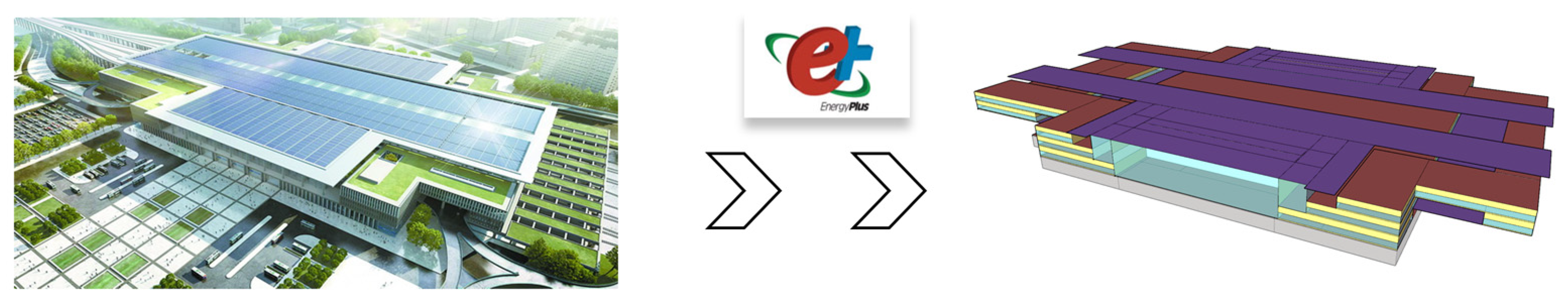
4.1. Case Description
4.2. Experimental Configuration
- Can the proposed method for constructing the training dataset in this paper support the offline optimization scheme and possess high computational efficiency?
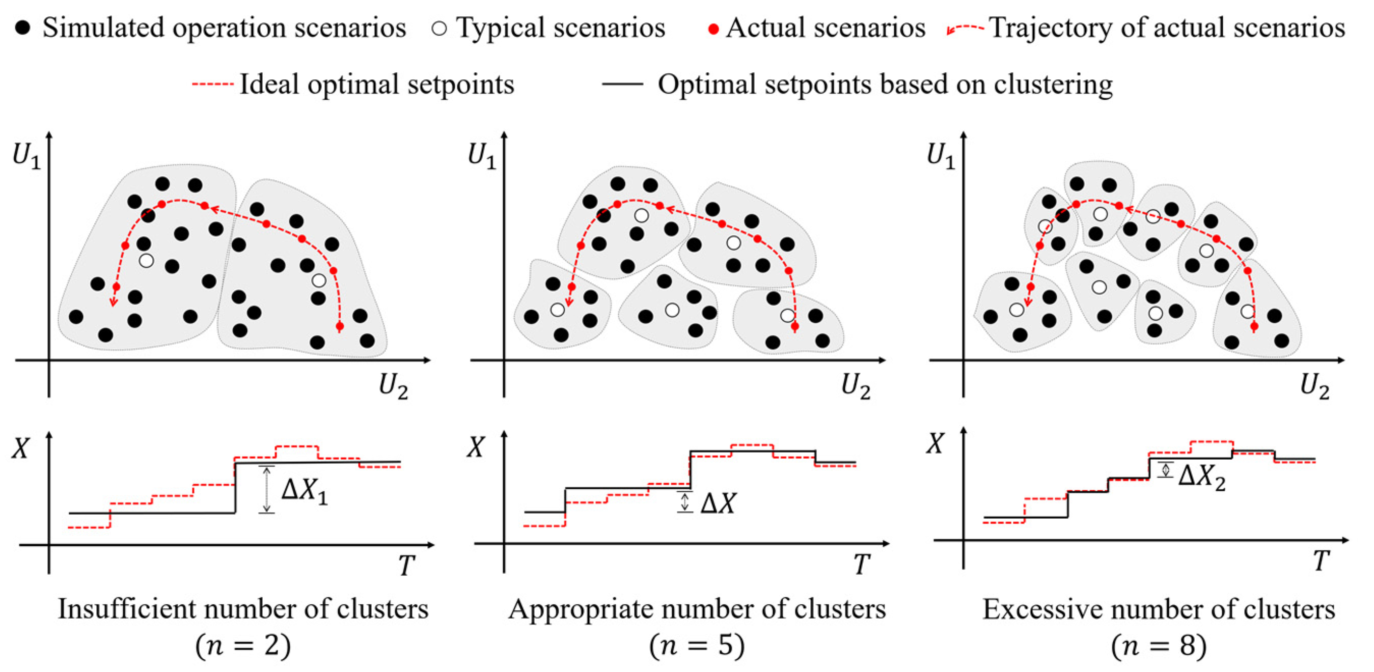
- How does the number of clusters in the dataset acquisition stage influence the performance of system optimization, and can the verification included in the second section effectively reflect this influence?
5. Results and Discussion
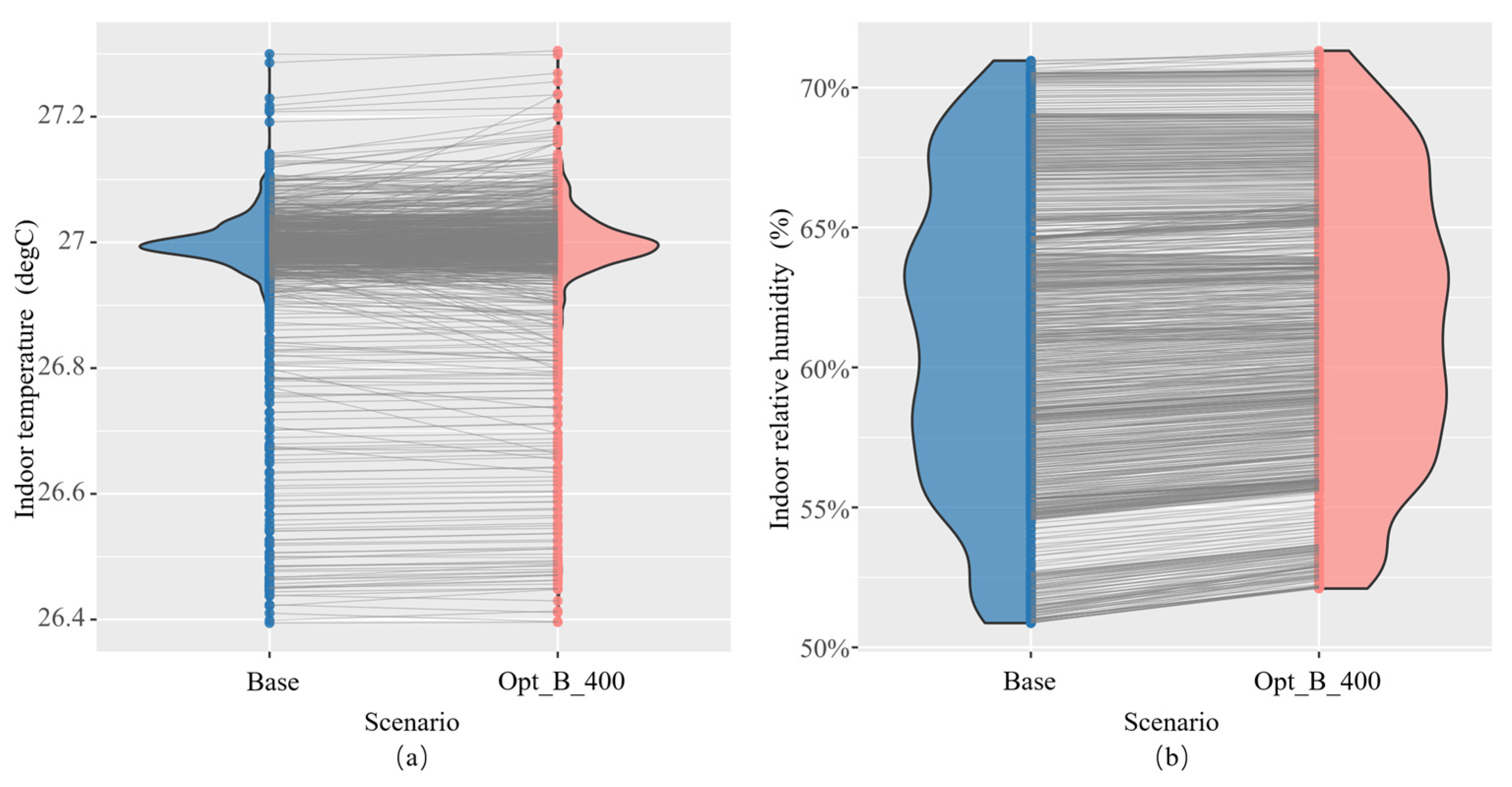
5.1. Optimized Control Effect Analysis
5.2. Analysis of the Efficiency in Dataset Acquisition
5.3. Analysis of the Rationality of Evaluation Metrics
6. Conclusions and Future Work
- This paper only considers the operation optimization of systems without energy storage where the temporal correlation between operation scenarios does not need to be paid much attention. However, when energy storage devices are involved, how to consider the temporal correlation between operation scenarios becomes a major issue.
- The generation of the simulated operation scenarios to be optimized proposed in this paper is based on deterministic meteorological boundaries and occupancy patterns provided in design documents. However, in practical engineering, such information is often uncertain. Therefore, it is important to investigate how the differences between actual and design information impact the acquisition of the training datasets, especially when dealing with uncertain boundaries.
Author Contributions
Funding
Conflicts of Interest
Nomenclature
| Nomenclature | Description |
|---|---|
| Outdoor dry-bulb temperature (°C) | |
| Outdoor relative humidity (%) | |
| Cooling load ratio (with maximum load as 100%) (%) | |
| Setpoint of temperature difference between supply and return chilled water (°C) | |
| Setpoint of temperature difference between supply and return cooling water (°C) | |
| Chiller outlet temperature setpoint (°C) | |
| Cooling tower outlet temperature setpoint (°C) | |
| AHU supply air temperature setpoint (°C) | |
| Indoor temperature setpoint (°C) | |
| Number of chillers in operation | |
| Number of cooling towers in operation | |
| Number of condenser water pumps in operation | |
| Number of chilled water pumps in operation |
Appendix A. Setting Parameters of the Optimization Algorithm
| Parameters | Value | Parameter | Value |
|---|---|---|---|
| Algorithm | GPSPSOCCHJ | CognitiveAcceleration | 2.7 |
| NeighborhoodTopology | vonNeumann | SocialAcceleration | 1.3 |
| NeighborhoodSize | 5 | MaxVelocityGainContinuous | 0.5 |
| NumberOfParticle | 49 | MaxVelocityDiscrete | 4 |
| NumberOfGeneration | 20 | ConstrictionGain | 0.5 |
References
- United Nations Environment Programme. 2021 Global Status Report for Buildings and Construction: Towards a Zero-Emission, Efficient and Resilient Buildings and Construction Sector; United Nations Environment Programme: Nairobi, Kenya, 2021. [Google Scholar]
- Pérez-Lombard, L.; Ortiz, J.; Pout, C. A review on buildings energy consumption information. Energy Build. 2008, 40, 394–398. [Google Scholar] [CrossRef]
- 2019 Global Status Report for Buildings and Construction; United Nations Environment Programme: Nairobi, Kenya, 2019; p. 41.
- Wang, S.; Ma, Z. Supervisory and Optimal Control of Building HVAC Systems: A Review. HVACR Res. 2008, 14, 3–32. [Google Scholar] [CrossRef]
- Drgoňa, J.; Arroyo, J.; Cupeiro Figueroa, I.; Blum, D.; Arendt, K.; Kim, D.; Ollé, E.P.; Oravec, J.; Wetter, M.; Vrabie, D.L.; et al. All you need to know about model predictive control for buildings. Annu. Rev. Control 2020, 50, 190–232. [Google Scholar] [CrossRef]
- Serale, G.; Fiorentini, M.; Capozzoli, A.; Bernardini, D.; Bemporad, A. Model Predictive Control (MPC) for Enhancing Building and HVAC System Energy Efficiency: Problem Formulation, Applications and Opportunities. Energies 2018, 11, 631. [Google Scholar] [CrossRef] [Green Version]
- Mariano-Hernández, D.; Hernández-Callejo, L.; Zorita-Lamadrid, A.; Duque-Pérez, O.; Santos García, F. A review of strategies for building energy management system: Model predictive control, demand side management, optimization, and fault detect & diagnosis. J. Build. Eng. 2021, 33, 101692. [Google Scholar] [CrossRef]
- Nguyen, A.-T.; Reiter, S.; Rigo, P. A review on simulation-based optimization methods applied to building performance analysis. Appl. Energy 2014, 113, 1043–1058. [Google Scholar] [CrossRef]
- Fu, Y.; Zuo, W.; Wetter, M.; VanGilder, J.W.; Han, X.; Plamondon, D. Equation-based object-oriented modeling and simulation for data center cooling: A case study. Energy Build. 2019, 186, 108–125. [Google Scholar] [CrossRef]
- Merema, B.; Saelens, D.; Breesch, H. Demonstration of an MPC framework for all-air systems in non-residential buildings. Build. Environ. 2022, 217, 109053. [Google Scholar] [CrossRef]
- Huang, S.; Zuo, W.; Sohn, M.D. Improved cooling tower control of legacy chiller plants by optimizing the condenser water set point. Build. Environ. 2017, 111, 33–46. [Google Scholar] [CrossRef] [Green Version]
- Haves, P.; Hencey, B.; Borrell, F.; Elliot, J.; Ma, Y.; Coffey, B.; Sorin, B.; Michael, W. Model Predictive Control of HVAC Systems: Implementation and Testing at the University of California, Merced; Lawrence Berkeley National Lab.(LBNL): Berkeley, CA, USA, 2010. [Google Scholar] [CrossRef] [Green Version]
- Campos, G.; Liu, Y.; Schmidt, D.; Yonkoski, J.; Colvin, D.; Trombly, D.M.; El-Farra, N.H.; Palazoglu, A. Optimal real-time dispatching of chillers and thermal storage tank in a university campus central plant. Appl. Energy 2021, 300, 117389. [Google Scholar] [CrossRef]
- Granderson, J.; Lin, G.; Blum, D.; Earni, S.; Page, J.; Piette, M.A. Optimizing Operational Efficiency: Integrating Energy Information Systems and Model-Based Diagnostics. In ESTCP Final Report: 201254; Lawrence Berkeley National Laboratory: Berkeley, CA, USA, 2017. [Google Scholar]
- Picard, D.; Jorissen, F.; Helsen, L. Methodology for Obtaining Linear State Space Building Energy Simulation Models. In Proceedings of the 11th International Modelica Conference, Versailles, France, 21–23 September 2015; pp. 51–58. [Google Scholar] [CrossRef] [Green Version]
- May-Ostendorp, P.; Henze, G.P.; Corbin, C.D.; Rajagopalan, B.; Felsmann, C. Model-predictive control of mixed-mode buildings with rule extraction. Build. Environ. 2011, 46, 428–437. [Google Scholar] [CrossRef]
- Domahidi, A.; Ullmann, F.; Morari, M.; Jones, C.N. Learning decision rules for energy efficient building control. J. Process Control 2014, 24, 763–772. [Google Scholar] [CrossRef]
- Klaučo, M.; Drgoňa, J.; Kvasnica, M.; Cairano, S.D. Building Temperature Control by Simple MPC-like Feedback Laws Learned from Closed-Loop Data. IFAC Proc. Vol. 2014, 47, 581–586. [Google Scholar] [CrossRef] [Green Version]
- Drgoňa, J.; Picard, D.; Kvasnica, M.; Helsen, L. Approximate model predictive building control via machine learning. Appl. Energy 2018, 218, 199–216. [Google Scholar] [CrossRef]
- Afram, A.; Janabi-Sharifi, F. Review of modeling methods for HVAC systems. Appl. Therm. Eng. 2014, 67, 507–519. [Google Scholar] [CrossRef]
- Wetter, M.; Wright, J. A comparison of deterministic and probabilistic optimization algorithms for nonsmooth simulation-based optimization. Build. Environ. 2004, 39, 989–999. [Google Scholar] [CrossRef] [Green Version]
- Tang, R.; Wang, S. Model predictive control for thermal energy storage and thermal comfort optimization of building demand response in smart grids. Appl. Energy 2019, 242, 873–882. [Google Scholar] [CrossRef]
- Kusiak, A.; Li, M.; Tang, F. Modeling and optimization of HVAC energy consumption. Appl. Energy 2010, 87, 3092–3102. [Google Scholar] [CrossRef]
- Kusiak, A.; Xu, G. Modeling and optimization of HVAC systems using a dynamic neural network. Energy 2012, 42, 241–250. [Google Scholar] [CrossRef]
- Afroz, Z.; Shafiullah, G.M.; Urmee, T.; Shoeb, M.A.; Higgins, G. Predictive modelling and optimization of HVAC systems using neural network and particle swarm optimization algorithm. Build. Environ. 2022, 209, 108681. [Google Scholar] [CrossRef]
- Magnier, L.; Haghighat, F. Multiobjective optimization of building design using TRNSYS simulations, genetic algorithm, and Artificial Neural Network. Build. Environ. 2010, 45, 739–746. [Google Scholar] [CrossRef]
- Perera, D.W.U.; Pfeiffer, C.F. Control of temperature and energy consumption in buildings—A review. Energy Environ. 2014, 5, 471–484. [Google Scholar]
- Afram, A.; Janabi-Sharifi, F. Theory and applications of HVAC control systems—A review of model predictive control (MPC). Build. Environ. 2014, 72, 343–355. [Google Scholar] [CrossRef]
- Baños, R.; Manzano-Agugliaro, F.; Montoya, F.G.; Gil, C.; Alcayde, A.; Gómez, J. Optimization methods applied to renewable and sustainable energy: A review. Renew. Sustain. Energy Rev. 2011, 15, 1753–1766. [Google Scholar] [CrossRef]
- Sun, F.; Yu, J.; Zhao, A.; Zhou, M. Optimizing multi-chiller dispatch in HVAC system using equilibrium optimization algorithm. Energy Rep. 2021, 7, 5997–6013. [Google Scholar] [CrossRef]
- Gao, Z.; Yu, J.; Zhao, A.; Hu, Q.; Yang, S. Optimal chiller loading by improved parallel particle swarm optimization algorithm for reducing energy consumption. Int. J. Refrig. 2022, 136, 61–70. [Google Scholar] [CrossRef]
- Zheng, Z.; Li, J.; Duan, P. Optimal chiller loading by improved artificial fish swarm algorithm for energy saving. Math. Comput. Simul. 2019, 155, 227–243. [Google Scholar] [CrossRef]
- Chen, S.; Liu, X.; Fu, H. Design of Energy-saving Optimized Remote Control System of Chiller Based on Improved Particle Swarm Optimization. In Proceedings of the 2018 5th IEEE International Conference on Cloud Computing and Intelligence Systems (CCIS), Nanjing, China, 23–25 November 2018; pp. 299–304. [Google Scholar] [CrossRef]
- Kusiak, A.; Xu, G.; Zhang, Z. Minimization of energy consumption in HVAC systems with data-driven models and an interior-point method. Energy Convers. Manag. 2014, 85, 146–153. [Google Scholar] [CrossRef]
- Castilla, M.; Álvarez, J.D.; Normey-Rico, J.E.; Rodríguez, F. Thermal comfort control using a non-linear MPC strategy: A real case of study in a bioclimatic building. J. Process Control 2014, 24, 703–713. [Google Scholar] [CrossRef]
- Åkesson, J.; Årzén, K.-E.; Gäfvert, M.; Bergdahl, T.; Tummescheit, H. Modeling and optimization with Optimica and JModelica.org—Languages and tools for solving large-scale dynamic optimization problems. Comput. Chem. Eng. 2010, 34, 1737–1749. [Google Scholar] [CrossRef]
- Drgona, J.; Helsen, L.; Vrabie, D.L. Cutting the Deployment Costs of Physics-Based MPC in Buildings by Simulation-Based Imitation Learning. In Proceedings of the ASME 2020 Dynamic Systems and Control Conference, Virtual, 5–7 October 2020. [Google Scholar] [CrossRef]
- Coffey, B. Approximating model predictive control with existing building simulation tools and offline optimization. J. Build. Perform. Simul. 2013, 6, 220–235. [Google Scholar] [CrossRef]
- Coffey, B.; Haghighat, F.; Morofsky, E.; Kutrowski, E. A software framework for model predictive control with GenOpt. Energy Build. 2010, 42, 1084–1092. [Google Scholar] [CrossRef]
- Wetter, M.; Zuo, W.; Nouidui, T.; Pang, X. Modelica Buildings library. J. Build. Perform. Simul. 2014, 7, 253–270. [Google Scholar] [CrossRef] [Green Version]
- Wetter, M.; Treeck, C.; Helsen, L.; Maccarini, A.; Saelens, D.; Robinson, D.; Schweiger, G. IBPSA Project 1, BIM/GIS and Modelica framework for building and community energy system design and operation—Ongoing developments, lessons learned and challenges. IOP Conf. Series Earth Environ. Sci. 2019, 323, 012114. [Google Scholar] [CrossRef]
- Wetter, M. GenOpt®—A Generic Optimization Program. In Proceedings of the Seventh International IBPSA Conference, Rio de Janeiro, Brazil, 13–15 August 2001. [Google Scholar]
- Hatledal, L.I.; Zhang, H.; Collonval, F. Enabling Python Driven Co-Simulation Models with PythonFMU. In Proceedings of the ECMS 2020 Proceedings; Communications of the ECMS, Berlin, Germany, 9–12 June 2020; Volume 34. [Google Scholar]


| Items | Parameters | Value |
|---|---|---|
| Building Construction and Occupancy | Wall conductivity | 0.34 W/(m2k) |
| Roof conductivity | 0.50 W/(m2k) | |
| Window conductivity | 2.2 W/(m2k) | |
| Heat gain coefficient of windows | 0.29 SHGC | |
| Window-to-Wall Ratio | East: 37% South: 35% West: 28% North: 37% | |
| Maximum occupancy | 14,000 people | |
| HVAC System | Chiller × 4 | Nominal Capacity: 5630 kW |
| IPLV: 9.364 | ||
| Design COP: 6.030 | ||
| Chilled water pump × 4 | Nominal flow rate: 1250 m3/h | |
| Nominal head: 33 mH2O | ||
| Nominal speed: 980 r/min | ||
| Nominal power: 160 kW | ||
| Condenser water pump × 4 | Nominal flow rate: 1250 m3/h | |
| Nominal head: 33 mH2O | ||
| Nominal speed: 980 r/min | ||
| Nominal power: 160 kW | ||
| Cooling tower × 16 | Nominal flow rate: 400 m3/h | |
| Nominal power: 12 kW | ||
| Cooling demand | Indoor temperature | 27 °C |
| Indoor relative humidity | <=70% |
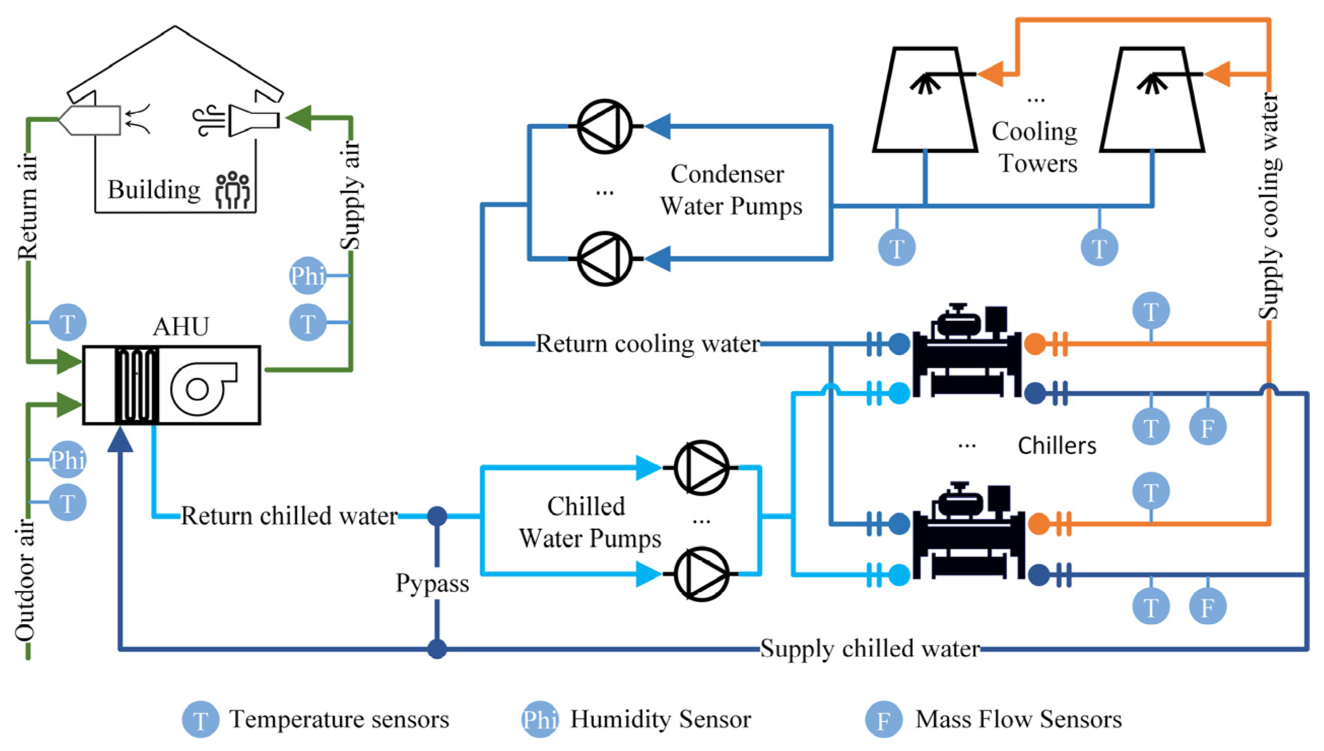
| Plant | Control Variables | Equipment-Level Controls | Original Strategy |
|---|---|---|---|
| Cooling tower | On/Off control | 1 chiller: 4 cooling towers * | |
| PID control | + 4 °C | ||
| Condenser water pump | On/Off control | 1 chiller: 1 pump | |
| PID control | 5 °C | ||
| Chiller | On/Off control | Load-based control | |
| PID control | 6 °C | ||
| Chilled water pump | On/Off control | 1 chiller: 1 pump | |
| PID control | 7 °C | ||
| AHU | PID control | 17 °C | |
| PID control | 27 °C |
| Strategy | Source Literature | Detailed Explanations |
|---|---|---|
| Baseline Strategy (Base) | - | Use the original setpoints in the design data |
| Optimization Strategy 1 (Opt_A) | [17,19,34] | Use the time series of the full cooling season as the boundary and as a virtual scenario for sequential optimization simulation, and the control interval is chosen as 30 min |
| Optimization Strategy 2 (Opt_B) | - | Use the method mentioned in Section 2 (the number of clusters are selected as 400, 350, 300, 250, 200, 150, 100, 80, 60, 40, 20). The number of clusters is marked after the name for ease of writing (e.g., the optimization group 2 with the number of clusters 400 will be written as Opt_B_400) |
| Optimization Strategy 3 (Opt_C) | [38] | Using the orthogonal grid generation method to generate operational scenarios, where the grid interval is selected in the following way:
|
| Strategy | Energy-Saving Rate | Non-Guaranteed Hours | Calculation Time/ Number of Optimizations Runs |
|---|---|---|---|
| Opt_A | 12.06 % | 5.9207 h | 20.6106 d/5391 reps |
| Opt_C | 11.50 % | 8.2602 h | 3.86439 d/1100 reps |
| Opt_B_400 | 11.62 % | 7.0561 h | 1.41498 d/400 reps |
Disclaimer/Publisher’s Note: The statements, opinions and data contained in all publications are solely those of the individual author(s) and contributor(s) and not of MDPI and/or the editor(s). MDPI and/or the editor(s) disclaim responsibility for any injury to people or property resulting from any ideas, methods, instructions or products referred to in the content. |
© 2023 by the authors. Licensee MDPI, Basel, Switzerland. This article is an open access article distributed under the terms and conditions of the Creative Commons Attribution (CC BY) license (https://creativecommons.org/licenses/by/4.0/).
Share and Cite
Tian, Z.; Ye, C.; Zhu, J.; Niu, J.; Lu, Y. Accelerating Optimal Control Strategy Generation for HVAC Systems Using a Scenario Reduction Method: A Case Study. Energies 2023, 16, 2988. https://doi.org/10.3390/en16072988
Tian Z, Ye C, Zhu J, Niu J, Lu Y. Accelerating Optimal Control Strategy Generation for HVAC Systems Using a Scenario Reduction Method: A Case Study. Energies. 2023; 16(7):2988. https://doi.org/10.3390/en16072988
Chicago/Turabian StyleTian, Zhe, Chuang Ye, Jie Zhu, Jide Niu, and Yakai Lu. 2023. "Accelerating Optimal Control Strategy Generation for HVAC Systems Using a Scenario Reduction Method: A Case Study" Energies 16, no. 7: 2988. https://doi.org/10.3390/en16072988