Multi-Time-Scale Coordinated Optimum Scheduling Technique for a Multi-Source Complementary Power-Generating System with Uncertainty in the Source-Load

Abstract

An optimal dispatching strategy for a multi-source complementary power generation system taking source–load uncertainty into account is proposed, in order to address the effects of large-scale intermittent renewable energy consumption and power load instability on power grid dispatching. The uncertainty problem is first converted into common situations for study, such as load power forecasting and solar and wind power. The backward scenario reduction and Latin hypercube sampling techniques are used to create these common situations. Based on this, a multi-timescale coordinated optimum scheduling control method for a multi-source complementary power generation system taking the demand response into account is presented, and the optimal operation of a wind–PV–thermal-pumped storage hybrid system is examined. The time-of-use power price optimizes the electrical load in the day-ahead pricing mode, and the two types of demand response loads are selected in the day-ahead scheduling. Second, the lowest system operating cost and the minimal day-ahead and intra-day adjustment of each source are established as the optimization targets in the day-ahead and intra-day phases of the multi-timescale coordinated scheduling model of the multi-source complementary system. The example study demonstrates that the scheduling strategy may increase the amount of renewable energy consumed, minimize load fluctuations, increase system stability, and further reduce operating expenses, proving the viability and efficiency of the suggested strategy.

1. Introduction

The functioning of the power system’s dispatching is made more difficult by the unpredictability posed by the expansion of availability to renewable energy sources such as wind and PV [1]. The main solutions to the issue of renewable energy consumption are to increase the consumption of renewable energy, depending on the complementary qualities of different power sources; combine various forms of variable resources; and maximize the performance of hybrid power systems. These strategies try to decrease the uncertainty associated with wind and PV power generation [2,3]. The large-scale combination of energy storage devices and renewable energy technologies is an effective means to absorb new energy and reduce the overall energy consumption of the system. As a scarce clean regulation resource, a pumped storage power station has a large capacity, fast response speed, and outstanding peak regulation effect. Together, wind power, PV power, thermal power, and pumped storage may increase the integration of renewable energy, increase system dependability, and reduce pollutant emissions. This is based on the combination of these two types of units. It is crucial to maximize the cost effectiveness and improve the hybrid system’s performance. In addition, the fluctuation of the demand-side load increases the difficulty of the operation and management of multi-source complementary power generation systems. The load curve can be improved by adding the demand response mechanism to the system scheduling to use the pricing signal or incentive signal to transfer or stop the load.

The issue of how to solve the problem of power system scheduling with source–load uncertainty and to reduce the impact of source–load uncertainty on power grid operation, so as to improve the economy and reliability of power grid operation, has become an urgent problem to be solved for a high proportion of wind power and photovoltaic access to the power grid system. Domestic and foreign scholars have conducted relevant research on this issue. The conventional method is to apply the deterministic method to deal with the randomness of renewable energy—that is, to use energy storage devices or conventional power sources to stabilize the fluctuations caused by renewable energy. A day-ahead multi-timescale scheduling technique for microgrids based on hybrid energy storage systems is suggested in one article [4]. The operation of renewable energy sources, load unpredictability, and the effects of fluctuating power on grid operation are all optimized by the hybrid energy storage system composed of batteries and supercapacitors. However, studies demonstrate that these scheduling techniques have issues such as high costs and significant inaccuracies. Some studies have proposed to express the actual output of wind power, photovoltaic, and load as the sum of the determined predicted value and uncertain predicted error [5], so that an optimization model with uncertain variables can be used to formulate a scheduling plan. Interval optimization, robust optimization, and stochastic optimization are all methods of optimization that take uncertainty into account. However, the economies of interval optimization and robust optimization are relatively poor, whereas stochastic optimization can more closely link the system cost to the system scheduling by using the probability distribution information of uncertain variables to the model [6]. Among them, by using sampling to determine the probability distribution of unknown variables, the stochastic optimization model based on scenario analysis creates a large number of deterministic scenarios from uncertain variables [7]. One group [8] suggests a random optimization control approach with energy storage and uses a random optimization model to simulate a typical wind power output scenario. In another article [9], a multi-timescale optimal scheduling strategy for an AC/DC hybrid microgrid based on the scenario analysis method is proposed. The uncertainty of wind power, photovoltaic, and load is simulated by scenario analysis technology, which effectively suppresses the power fluctuation caused by multiple uncertainties of the microgrid. In another [10], the scenario analysis approach is used to determine how electric vehicles would affect the best power grid dispatch. In another article [11], considering the influence of the uncertainty of wind and solar output on the optimization of regional integrated energy system, combined with the model predictive control theory, the output of the unit is adjusted via correction and rolling optimization to achieve the coordinated operation of multiple timescales. The above research on the uncertainty of wind power, photovoltaic, and load fluctuation still has the following shortcomings: (1) most of the above literature is based on energy storage technology to stabilize power fluctuations at multiple timescales, and few models and analyses of uncertain variables are carried out; (2) most of the existing research objects focus on the analysis of small and medium-sized power generation systems such as microgrids, active distribution networks, and park-integrated energy. There are few applications for joint system planning involving large-scale wind power, photovoltaic grid-connected, and pumped storage energy storage units.

On the other hand, for the wind and solar consumption of the multi-source combined power generation system under a high proportion of renewable energy grid connection, the wind and solar fluctuations are mainly suppressed by optimizing the energy structure and increasing the energy storage device. One study [12] looked at maximizing the benefits of the joint operation of wind power, thermal power, and pumped storage, and considered the robust optimization strategy of multiple scenarios in different seasons to reduce the operating cost of the system. Based on the coordinated complementary mechanism of photovoltaic–energy storage, one group [13] dynamically adjusted the maximum power tracking operating point to suppress photovoltaic power fluctuations. In another work [14], for wind power and pumped storage, a combined dispatching optimization technique is recommended. A coordinated dispatching model is created to lessen wind curtailment, and this model serves as the conceptual framework for the creation of a wind power output system. As evidenced by the joint operating plan for pumped storage and a wind–PV complementary power generation system suggested in one paper [15], the addition of pumped storage may effectively suppress or compensate for the discrepancy between the output of wind–PV power generation and the expected output. In addition, for the scheduling strategy of renewable energy such as wind power and photovoltaic, many previous studies have focused on the short-term optimal scheduling technology of hybrid power systems [16,17]. The research on the coordinated operation of the two-resource hybrid power generation systems mainly includes a wind–solar complementary system, hydro–photovoltaic hybrid power generation system, and a hydro–wind hybrid power generation system. A day-ahead optimum scheduling model for wind–PV complementary power production with a unit spinning reserve and reservoir capacity as constraints is constructed in one article [18], which also studies the optimal functioning of wind–PV–pumped storage complementary power generation systems. The ideal day-ahead scheduling of hybrid power systems, which include thermal power, pumped storage, wind power, and PV power generation, was explored in another paper [19]. A day-ahead optimum scheduling model of a multi-source complementary power generating system is designed to optimize economic advantages and renewable energy consumption by taking into account the complementary properties of various power sources. In another article [20], considering the regulation of the demand-side load, an optimal scheduling model of renewable energy and energy storage device coordination is constructed. It shows that the introduction of the demand response can effectively realize the coordination of multiple types of energy and load, and provide differentiated energy consumption forms according to the different needs of users, so as to achieve efficient energy utilization. Another group [21] considers the ultra-short-term power prediction method of renewable energy, and establishes an intra-day rolling optimization model with minimum active power deviation and maximum wind power consumption. Based on the idea of step-by-step refinement, one group [22] established a multi-timescale scheduling model of source–storage–load considering the distribution characteristics of energy storage, which can reduce the operation cost of the system and improve the wind–solar accommodation capacity. The above research on renewable energy scheduling strategies still has the following shortcomings: (1) the coordinated regulation of pumped storage, wind power, and photovoltaic at different timescales is not considered in the joint operation optimization scheduling problem of pumped storage and renewable energy; (2) the traditional open-loop scheduling process represented by the refined time scale does not consider the feedback correction of the actual system to the optimal control process.

In summary, on the basis of considering the uncertainty of source–load, this paper proposes a multi-timescale optimal scheduling method for hybrid power systems including wind power, photovoltaic, thermal power, and pumped storage power generation, considering the demand response, by fully exploiting the complementary operation characteristics of various energy sources. The day-ahead and intra-day optimal scheduling model of a multi-source complementary system is established, and the coordinated scheduling model of the joint system is extensively studied. The complementary operation is realized by accurate joint scheduling, which provides a reference for the future demand response project of multi-source complementary power generation systems. Compared with the concepts of virtual power plants (VPPs) [23] and integrated energy systems (IES) [24], the proposed system effectively alleviates the power fluctuation on the power supply side while ensuring the economic operation of the multi-source complementary system. For simplicity, the main contributions and innovations of this paper are as follows.

(1)

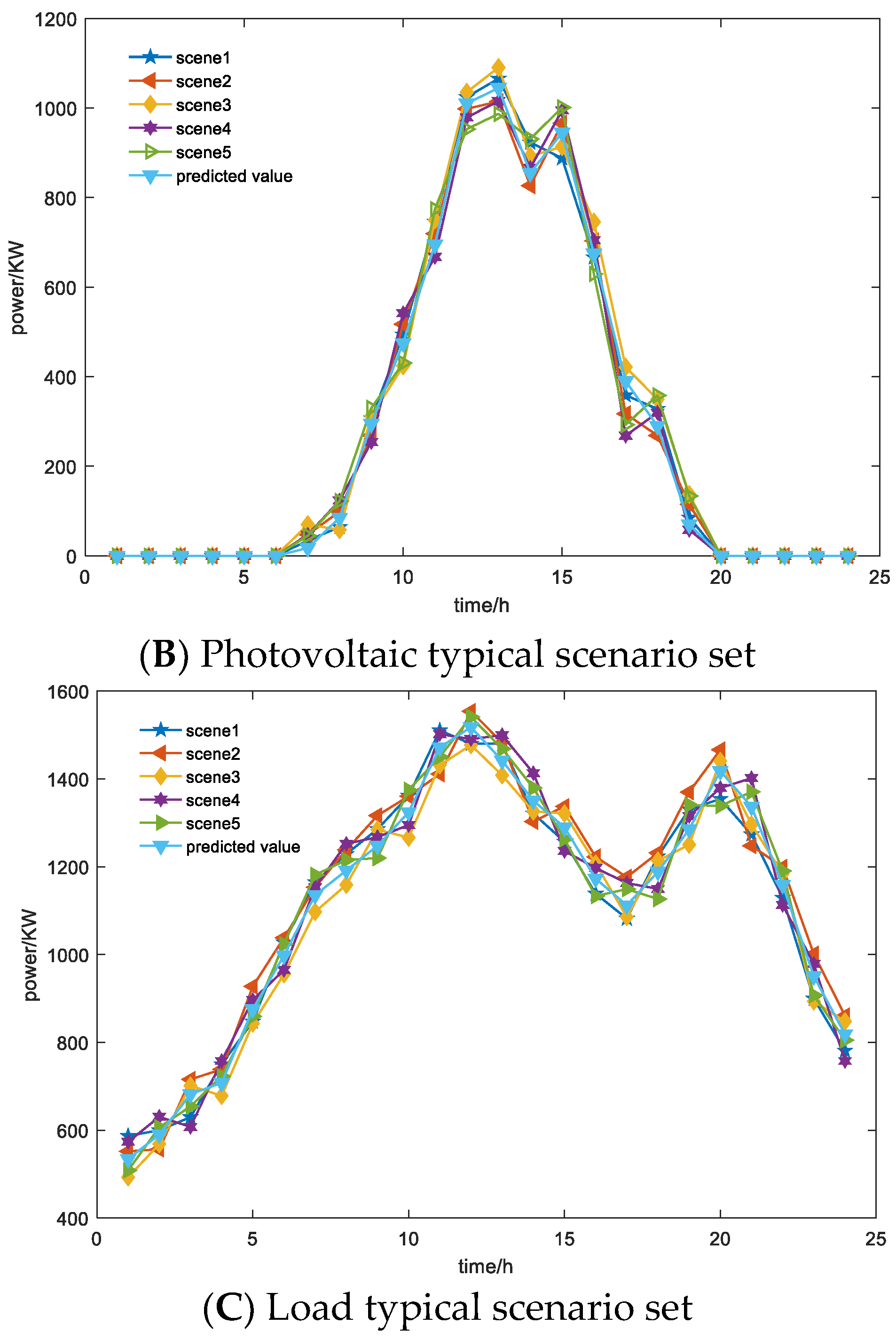
The influence of uncertain factors such as wind power, photovoltaic, and load is considered in the day-ahead stage. The power balance equation with uncertain variables in multiple scenarios is established, and the typical scenarios of wind power, photovoltaic, and load power prediction are generated by Latin hypercube sampling and backward scenario reduction technology. At the same time, the complementary operation characteristics of wind, photovoltaic, thermal power units, and pumped storage are analyzed, and the coordinated scheduling framework for the multi-source complementary system is proposed according to different operation characteristics. We provide scheduling strategies for multi-source complementary systems with pumped storage.

(2)

A multi-timescale coordinated scheduling strategy for multi-source complementary systems is proposed. In the day-ahead stage, the minimum operating cost of the system is taken as the optimization objective. In the intra-day stage, a rolling scheduling model based on ultra short-term forecast data is proposed, and the minimum day-ahead and intra-day adjustment of each source is taken as the optimization objective. Considering various constraints, such as the system power balance, pumped storage capacity, spinning reserve capacity, and demand response load, a multi-timescale coordinated optimization scheduling model for the multi-source complementary system is constructed.

(3)

According to the advantages of the demand response, we fully consider the interaction between the multi-source complementary power generation system and load demand side. A pricing and incentive demand response model based on market elasticity is created. The day-ahead scheduling and the introduction of the transferable load and interruptible load into the multi-source complementary system’s optimum scheduling model are considered. A future demand response project for a multi-source complementary system can use this analysis of the system’s overall impact of energy supply and demand as a guide.

The remaining sections of this paper are as follows. The construction of the multi-source complimentary system power generating system, each unit’s mathematical model, and the wind–PV–load uncertainty modeling are all introduced in Section 2. Section 3 describes the day-ahead and intra-day scheduling models. Section 4 covers many numerical simulations and describes case examples. Section 5 contains the conclusions.

2. Structure and Mathematical Model of Multi-Source Complementary Power Gene-Ration System

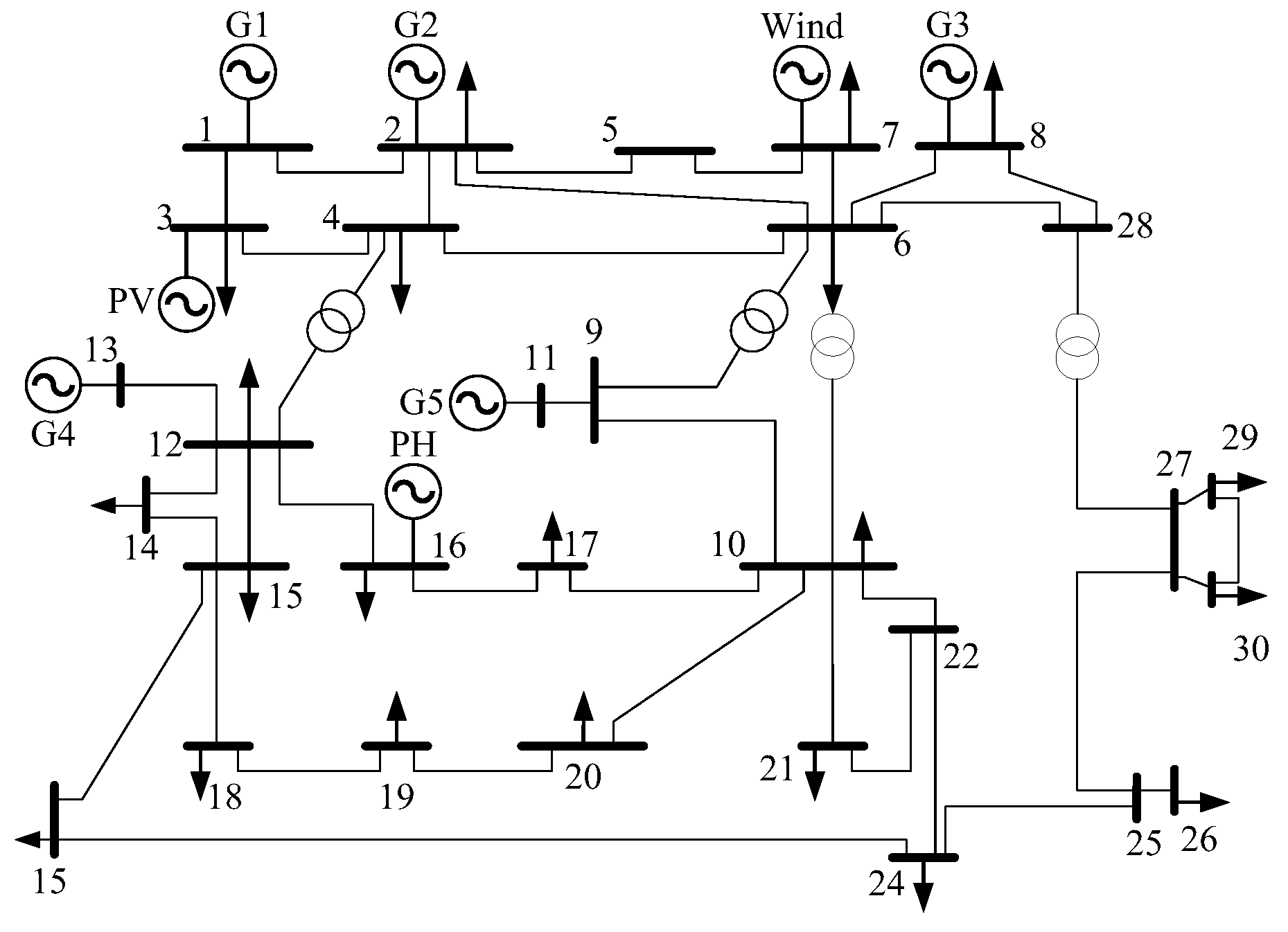
2.1. System Structure

The wind farm, photovoltaic power station, thermal power plant, pumped storage power station, power load, and dispatching center compose the multi-source complementary power generating system built in this article. The architecture of the system is shown in Figure 1. The output coordination between wind, PV, thermal, and other units is referred to as the multi-source complementary power generating system’s output characteristics. To minimize the uncertainty of wind and PV output and anti-peaking characteristics, and to track the imbalance between the wind and PV output curve and the load curve of the receiving end area, daily complementary output characteristics—that is, by adjusting the output of each unit and fully utilizing the adjustment ability of thermal power units—are achieved. This results in a more closely matched relationship between the delivery curve and the load curve of the receiving end area.

In the system, thermal power generation, wind turbines, and photovoltaic arrays are the main energy sources; pumped storage is used as a storage medium, and the grid is used as a backup (the grid cannot be used for storage). Due to the variability of renewable energy generation, there are excess and insufficient generation periods associated with the load. A portion of the power produced by the power producing side is sent to pumped storage to be stored as potential energy, while another portion is used for direct grid connection. Through the pump turbine, the pumped storage power plant switches the higher and lower reservoirs. The pump is initiated to pump water for energy storage when the power generated by the power producing side is more than the demand of the load end. While the system is operating at peak load, we start the turbine discharge to compensate for the lack of output. Once the lower limit of thermal power generation is reached, renewable power generation is activated as a priority.

2.2. Thermal Power Output Characteristics

The production of thermal power is variable within a particular range, independent of the weather or other effects, and highly controllable. The minimal technical output tends to be situated between the minimum and maximum output, which may be as low as 30% of the installed capacity [25]. The following formula splits the power regulation direction of thermal power units into uphill and downhill.

$$\{\begin{array}{c}{c}_i\ge {\beta }_{i,m}+{\alpha }_{i,m}\left(P_{T-i}-p_{i,m}\right)\\ U_{it}{P}_{i-min}\le P_{T-it}\le U_{it}{P}_{i-max}\\ -R_i^d\Delta t{U}_{it}-P_{i-max}\left(1-U_{it}\right)\le P_{it}-P_{i\left(t-1\right)}\le R_i^u\Delta t{U}_{i\left(t-1\right)}+P_{i-min}\left(1-U_{i\left(t-1\right)}\right)\end{array}$$

(1)

In the $t$ period, $c_i, {\beta }_{i,m}$, and ${\alpha }_{i,m}$ are the fuel cost, fixed cost, and variable cost coefficient of the unit; $P_{T-i}$, $p_{i,m}$ are the output value of the unit and the left end of the m segment; $U_{it}$ is the power on state of the unit, indicated by 0, 1; $P_{i-min}$ and $P_{i-max}$ are the lower and upper limit values of the unit’s output; $R_i^d, R_i^u$ is the hourly landslide and climbing power of the unit; $\Delta t$ is the time interval.

2.3. Mathematical Model of Pumped Storage Unit

The pumped storage units can start and stop and switch between different working conditions in a short period of time, and they have the characteristics of flexible adjustment and frequency regulation. The operation mode is to store electricity when the power load is at a low ebb and generate electricity at a peak. The residual power is utilized to operate the pump and transfer the water to the upper reservoir when the generation of renewable energy power in the multi-source complementary system exceeds the load on a daily regulated time scale. The turbine starts and powers the load when the demand for the load cannot be fulfilled by the renewable energy power output. The minimum output power of the turbine is set to 15% of the rated capacity [26], which is also the minimum output power of the pump. The volume expression for the upper and lower reservoir pools using the pump flow, turbine flow, and pumped storage unit is as follows:

$$\{\begin{array}{c}{Q}_p\left(t\right)=K_p\ast E_p\left(t\right)\\ Q_g\left(t\right)=E_t\left(t\right)\ast K_t{}^{-1}\\ V_t^{up}=V_{t-1}^{up}-Q_g\left(t\right)+\left(1-\alpha \right)Q_p\left(t\right)\\ V_t^{down}=V_{t-1}^{down}-Q_p\left(t\right)+\left(1-\beta \right)Q_g\left(t\right)\end{array}$$

(2)

Here, $Q_p\left(t\right)$, $Q_g\left(t\right)$ are the pump flow rate and the turbine power generation flow, m³/h; $E_p\left(t\right)$, $E_t\left(t\right)$ are the energy input pump and the power generated by the turbine, MWh; $K_p$, $K_t$ are the pumping and power generation coefficients of the pump turbine. At time t and time t − 1, the upper and lower reservoirs’ water volumes are $V_t^{up}$, $V_t^{down}$, and $V_{t-1}^{up}$, $V_{t-1}^{down}$, respectively; $\alpha$ and $\beta$ are the pumped storage unit’s respective water loss coefficients for power production and pumping.

2.4. Wind Power–Photovoltaic–Load Uncertainty Model in Multiple Scenarios

In this study, scenario analysis is utilized to examine forecasts for wind, photovoltaic, and load power.

Wind speed and wind power generation are connected. Weibull distribution is utilized in this study to model the uncertainty of wind power output and represent the variation in wind speed. According to its probability density function [27], the wind power output is modeled as shown below.

$$P_{w,t}=\{\begin{array}{c}0, v<v_i,v\ge v_o\\ P_w\frac{v-v_i}{v_r-v_i},v_i\le v\le v_r\\ P_w, v_r\le v<v_o\end{array}$$

(3)

Here, in the t period, the $P_{w,t}$, and $P_w$ are the output power and total installed capacity of the unit, kW; $v_i$, $v_o$, and $v_r$ are the cut into wind speed, cut out wind speed, and rated wind speed, m/s, respectively.

The photovoltaic intensity is linked to the output power characteristics of photovoltaic power generation. The probability distribution model of irradiance in this study is described using the beta distribution. The output power of photovoltaic power generation is modeled according to its probability density function:

$$P_{v,t}=\frac{\Gamma \left(\alpha +\beta \right)}{\Gamma \left(\alpha \right)+\Gamma \left(\beta \right)}{\left(P_{v,t}/P_{v,t}^{max}\right)}^{\alpha -1}{\left(\frac{r_{max}-r}{r_{max}}\right)}^{\beta -1}$$

(4)

Here, $P_{v,t}$ is the photovoltaic power during t period, kW; $\Gamma (·)$ is the gamma function; $\alpha$, $\beta$ are shape parameters of beta distribution; $P_{v,t}^{max}$ is the greatest photovoltaic output power in t period; $r$, $r_{max}$ are the photovoltaic radiation intensity and maximum radiation intensity, kw/m².

The probability density function is as follows, since the load’s variation follows the normal distribution [28]:

$$f\left(\Delta P_L\right)=\raisebox{1ex}{$e^{-\frac{{(\Delta P_L-\mu )}^2}{2{\delta }^2}}$}\!\left/ \!\raisebox{-1ex}{$\delta \sqrt{2\pi }$}\right.$$

(5)

Here, $\Delta P_L$ is the load fluctuation power; $\mu$ and ${\delta }^2$ are the expectation and variance of a normal distribution, respectively.

Based on the above uncertainty model, this paper uses Latin hypercube sampling (LHS) to generate a large number of random scenes [29]. The specific steps are as follows.

Step 1: Let X be an M-dimensional (M = 1,2,…, N) random variable. $Y_i=F_i$ is the formula for the probability distribution function of wind power, photovoltaic power, and load power, where i = 1, 2,…, M, and $Y_i$ is the function for the probability distribution of wind power, photovoltaic power, and load power.

Step 2: Extract L samples in each element, and obtain the jth sampling $x_{mj}$ of the mth element, where j = 1,2,…, L.

Step 3: The extracted samples are randomly combined to obtain the L × N dimensional sampling matrix $B=\left[v_i,c_j,e_k\right]$ of wind power, photovoltaic, and load power uncertainty. Among them, $v_i=\left[v_{i1},v_{i2},\dots ,v_{iL}\right]$, $c_j=\left[c_{j1},c_{j2},\dots ,c_{jL}\right]$, $e_k=\left[e_{k1},e_{k2},\dots ,e_{kL}\right]$ are the lth sampling data of wind speed, photovoltaic intensity, and load power, respectively.

Considering that the generation of a large number of scenes will increase the burden of solving operations, in order to reduce the amount of calculation, the backward scene reduction technology is used to reduce similar scenes. The reduced typical scene set can well reflect the probability distribution of the original scene set. The specific steps are as follows:

Step 1: Let the original scene set be B, and the scene set J that needs to be reduced in the number of iterations is an empty set. Calculating the scene distance of any two scenes forms the scene distance matrix $D[w\left(S_i\right),$ $w\left(S_j\right)]=\Vert w\left(S_i\right), w{\left(S_j\right)\Vert }_2$, where $w\left(S_i\right)$ is the uncertainty scene, $S_i$ and $S_j$ are scene numbers, and ‖$·$‖ is the Euclidean distance operator of vector space.

Step 2: The minimal distance probability $P_{Di}$ of the closest scene $S_k$ to the scene $S_i$ is calculated using the assumption that the likelihood of the scene Si occurring is $p_i$. $P_{Di }$ = $p_{i}min\left\{D\left[w\left(S_i\right), w\left(S_j\right)\right]\right\}$.

Step 3: Find the minimum $p_{Db}=min{P}_{Di}$ in all the current scene sets C, where $p_{Db}$ is the minimum distance probability of searching $S_i$ nearest scene $S_k$ in all scene sets C.

Step 4: Update the scene set B and plan to reduce the scene set J, and update the scene probability $p_i$ = $p_i$ + $p_{Db}$.

Through Latin hypercube sampling, a set of 10,000 day-ahead scenarios is generated. After backward reduction technology, the number of scenarios for wind power, photovoltaic output, and load power is 5, which is used to reflect the uncertainty of wind power, photovoltaic, and load. The power situation in each scenario is shown in Figure 2.

3. Multi-Timescale Coordinated Optimal Scheduling Model

3.1. Optimal Strategy

The prediction accuracy of wind and photovoltaic output will be improved step-by-step according to the continuous approximation of the timescale, and the disturbance to the system will be smaller. Therefore, the optimal scheduling on multiple timescales, through the timescale refinement, is achieved through step-by-step coordination to enhance the ability to accept renewable energy. The multi-source complementary power production system’s optimal scheduling strategy diagram for the day-ahead and the intra-day cases is shown in Figure 3.

(1)

The impact of wind, PV, and load power unpredictability on scheduling is taken into account in the day-ahead scheduling plan. Based on the scenario analysis method, the uncertainty model of wind–PV–load is established to optimize the day-ahead output. The time scale is set to 1 h, with a total of a 24 h execution cycle, and before the conclusion of the first day, a day-ahead scheduling plan for 24 periods on the second day is created based on the short-term forecast value. Determining the short-term forecast value of wind power and PV production is crucial for day-ahead scheduling; we obtain the short-term prediction value of user load power consumption, the output value of each unit and its cost of operation, the call plan of the PDR load response, and the IDR load, and input them into the intra-day rolling optimization scheduling as the determined quantity.

(2)

The variance between the wind–PV–load ultra short-term forecast data and the reference value is determined in the intra-day rolling scheduling plan based on the anticipated scheduling value of multi-scenario optimization scheduling. We set the time scale to 15 min, with a total of 4 h execution cycles and a total of 96 executions within a day, with a known ultra short-term forecast value continuously rolling correction day generation plan. All rolling schedules for the remaining five periods with the minimum load error of the day are developed during the last period ending in the first 4 h before the day. In order to correct the discrepancy between the day-ahead scheduling plan and the actual situation, intra-day rolling scheduling must be used to calculate the ultra-short-term prediction value of wind power and photovoltaic output; the ultra-short-term prediction of user load power consumption, the daily production of each unit, and the output of each unit before the day are used as the target quantities. In the final 15 min of the entire scheduling plan, the positive and negative spinning reserve capacity of the unit that the system ultimately calls is established. This is carried out to ensure that the system accurately predicts information and creates a spinning reserve plan to lower the spinning reserve cost.

(3)

The day-ahead scheduling plan serves as the foundation for the intra-day rolling optimization scheduling, which is based on it. The MPC method is used to carry out rolling optimization for 96 periods during the day based on the ultra-short-term forecast information of wind power and photovoltaic power output, in order to effectively reduce the amount of intra-day adjustment of each source while ensuring the effectiveness of the day-ahead scheduling plan and minimizing the impact of the day-ahead scheduling plan.

The characteristics of the prediction information related to the timescale (the shorter the timescale, the higher the prediction accuracy) are used to formulate a more accurate scheduling plan through the multi-timescale coordinated optimal scheduling strategy of multi-source complementary systems, and the complementary adjustment is realized by fully utilizing the source–load coordination characteristics, boosting the use of renewable energy as a result.

3.2. Demand Response Model

The demand response is separated into price-based and incentive-based segments depending on the various user response strategies. This study presents the demand response (DR) to optimize the electric load in accordance with time-of-use prices, adopts price-based DR, achieves electric load transfer using a transferable load, and modifies the transferable load in peak hours to the period of energy price underestimation. In order to fulfill the goals of smoothing the load curve, peak load shifting, and enhancing the dependability of the system, the interruptible load in the peak period is compensated using the incentive demand response. In order to optimize the power load, the model adopts the day-ahead pricing mode and describes how the grid price signal affects users’ electricity consumption patterns using the price elasticity coefficient of the time-of-use electricity price. The day-ahead scheduling determines the two forms of demand response loads.

3.2.1. Day-Ahead Load Model Based on PDR

In this paper, the elastic matrix method of electricity price elasticity is used to model the response of the electric load, and its index is used to express the rate of change of the electric load and electricity price, i.e., to direct users to reasonably adjust their electricity strategy through the time-of-use price. Based on the elasticity coefficient and elasticity matrix [30], the transferable load model of users in the i period is

$$P_{SL,i}=P_{SL,i}^0\left(1+{\displaystyle \sum }_{j=1}^{24}\frac{E_{SL}\left(i,j\right)\Delta Q_j}{Q_j^0}\right)$$

(6)

where $P_{SL,i}^0$ is the initial value of the transferable load; $E_{SL}\left(i,j\right)$ is the price demand elasticity matrix; $Q_j^0$ and $\Delta Q_j$ are the initial electricity price and the change in electricity price; the value range of time period i and j is 1~24.

3.2.2. Day-Ahead Load Model Based on IDR

The interruptible load is expressly referred to as the IDR response type in this study. The interruptible load’s response procedure involves responding to the dispatching center’s interruption request in a certain amount of time in order to meet the goals of reducing the operational pressure on the system and obtaining a particular financial reward. Economic compensation generally includes capacity compensation and power compensation, as shown in a previous study [31]. The electrical load expression after user n adopts an interruptible load in i period is as follows:

$$P_{IL,i}=P_{IL,i}^0-{\sum }_{n=1}^{N_{IL}}{\epsilon }_{n,i}{P}_{IL-i,n}$$

(7)

where $P_{IL,i}^0$ and $P_{IL,i}$ are the electrical load requirements before and after the use of interruptible loads; ${\epsilon }_{n,i}$ is the interrupt state variable, represented by 0 and 1, where the value of 1 indicates the interrupt state, and the value of 0 indicates that the load is not interrupted; $P_{IL-i,n}$ is the interruptible load value; and $N_{IL}$ is the number of interruptible users.

3.3. Day-Ahead Stochastic Optimal Scheduling Based on Multi-Scenario Technology

3.3.1. Objective Function

The day-ahead scheduling plan aims to minimize the system cost, and its expression is as follows:

$$\{\begin{array}{c}F=min{\sum }_{t=1}^T\left\{{\sum }_{i=1}^{N_T}{U}_{it}\left[f\left(P_{T-it}\right)+S_{it}\left(1-U_{i\left(t-1\right)}\right)+C_{ri}\left(R_{it}^u,R_{it}^d\right)\right]+{\sum }_{k=1}^{N_H}\left(S_{kt}^{gen}+S_{kt}^{pum}\right)\right\}\\ f\left(P_{T-it}\right)=a_i{P}_{T-it}^2+b_i{P}_{T-it}+c_i\\ C_{ri}\left(R_{it}^u,R_{it}^d\right)=k_{it}^u{R}_{it}^u+k_{it}^d{R}_{it}^d\\ S_{kt}^{gen}=S_k^{gen}{I}_{kt}^{gen}\left(I_{kt}^{gen}-I_{k\left(t-1\right)}^{gen}\right)\\ S_{kt}^{pum}=S_k^{pum}{I}_{kt}^{pum}\left(I_{kt}^{pum}-I_{k\left(t-1\right)}^{pum}\right)\end{array}$$

(8)

Here, $U_{it}$ shown as 1, 0, and is the ith thermal power unit’s start–stop condition; $S_{it}$ is the start-up cost of thermal power units; T is the total number of time periods, taken as 24; $N_T$ is the total number of thermal power units; $N_H$ is the total number of pumping and storage units; $f\left(P_{T-it}\right)$ is the cost of generating electricity from thermal power units; $P_{T-it}$ is the output value of the thermal power unit; $a_i$, $b_i$, and $c_i$ are the correlation coefficients of the operating costs of thermal power units; $C_{ri}\left(R_{it}^u,R_{it}^d\right)$ is the spare cost of thermal power units. The thermal power unit’s positive and negative spinning reserves are represented by $R_{it}^u$ and $R_{it}^d$ in the time period; the positive and negative reserve costs of thermal power units are known as $k_{it}^u$ and $k_{it}^d$. When the value of $I_{kt}^{gen}$ is 1, it indicates that the pumped storage unit is in the power generation condition in period t; $S_{kt}^{gen}$ is the start-up cost of the pumping unit k in the power generation condition during the t period; $S_k^{gen}$ is the start-up cost of the pumping and storage unit when it is in the power generation condition. When the value of $I_{kt}^{pum}$ is 1, it signifies that the pumped storage unit works in the pumping condition for the duration of the specified time period. $S_k^{pum}$ denotes the start-up cost of the pumping condition of the kth pumped storage unit.

3.3.2. Constraint Condition

Power Balance Constraint

In order to ensure the safe and stable operation of the power grid, it is necessary to maintain a balance between supply and demand, between the total power and load demand. The existing grid power balance constraints are mostly based on the prediction data of renewable energy sources and loads such as wind power and photovoltaics. In order to facilitate the model solution, the prediction error is directly ignored, as shown in Equation (9).

$${\sum }_{x=1}^{N_W}{P}_{W-xt}+{\sum }_{y=1}^{N_V}{P}_{V-yt}+{\sum }_{i=1}^{N_T}{P}_{T-it}+{\sum }_{k=1}^{N_H}{P}_{H-kt}=P_{Lt}^{pre}+\Delta PD{R}_t+\Delta ID{R}_t$$

(9)

At the t moment, $P_{W-xt}$, $P_{V-yt}$, $P_{T-it}$, and $P_{H-kt}$ indicate the output of wind turbines, photovoltaic units, thermal power units, and pumped storage units, respectively. $N_W$, $N_V$, $N_T$, and $N_H$ are the total number of wind turbines, photovoltaic units, thermal power units, and pumped storage units, respectively; a $P_{H-kt}$ value greater than zero reflects the power generation condition, and less than zero reflects the pumping condition; $P_{Lt}^{pre}$ is the forecast value of the electricity load; $\Delta PD{R}_t$ and $\Delta ID{R}_t$ are load response quantities.

In this paper, the power balance equation considering the uncertainty of wind power, photovoltaic, and load is shown in Equation (10). The actual values of wind power, photovoltaic output, and load power are expressed by the sum of the predicted value and prediction error.

$${\sum }_{x=1}^{N_W}\left(P_{W-xt}+{\epsilon }_{w,x}\right)+{\sum }_{y=1}^{N_V}(P_{V-yt}+{\epsilon }_{v,y})+{\sum }_{i=1}^{N_T}{P}_{T-it}+{\sum }_{k=1}^{N_H}{P}_{H-kt}=\left(P_{Lt}^{pre}+{\epsilon }_L\right)+\Delta PD{R}_t+\Delta ID{R}_t$$

(10)

Here, ${\epsilon }_{w,x}$, ${\epsilon }_{v,y}$, and ${\epsilon }_L$ are the prediction errors of wind power, photovoltaic output, and load power, respectively.

Due to the uncertainty of wind power, photovoltaic output, and the load power prediction error, Equation (10) cannot be solved directly. In this paper, the scenario analysis method is used to quantify it. According to the probability distribution function of wind power, photovoltaic output, and load power fluctuation, multiple scenarios are generated, which requires the balance of the supply and demand of electric energy in each scenario. $P_{W-xt}^s+{\epsilon }_{w,x}$ is used to represent the actual output of wind turbines under scenario s, $P_{V-yt}^s+{\epsilon }_{v,y}$ is used to represent the actual output of photovoltaic under scenario s, and $P_{Lt}^s+{\epsilon }_L$ is used to represent the total load power under scenario s. The stochastic optimization model with uncertain variables is transformed into a deterministic model for processing. The power balance equation is shown in Equation (11):

$${\sum }_{x=1}^{N_W}\left(P_{W-xt}^s+{\epsilon }_{w,x}\right)+{\sum }_{y=1}^{N_V}\left(P_{V-yt}^s+{\epsilon }_{v,y}\right)+{\sum }_{i=1}^{N_T}{P}_{T-it}+{\sum }_{k=1}^{N_H}{P}_{H-kt}=P_{Lt}^{pre}+{\epsilon }_L$$

(11)

Wind and Photovoltaic Output Constraints

It should be assured that the on-grid power of wind and PV is lower than its expected value in the present situation before the day-ahead scheduling plan of the system is developed. The output constraint is

$$\{\begin{array}{c}0\le P_{W-t}\le P_{W-t}^{pre}\\ 0\le P_{V-t}\le P_{V-t}^{pre}\end{array}$$

(12)

Here, the short-term forecast values for wind and photovoltaic output at time t are $P_{W-t}^{pre}$, and $P_{V-t}^{pre}$.

Thermal Power Unit Constraints

The following are the minimum start-up and shutdown time restrictions for thermal power units:

$$\{\begin{array}{c}{T}_{it}^{on}\ge T_{imin}^{on}\\ T_{it}^{off}\ge T_{imin}^{off}\end{array}$$

(13)

The thermal power units’ starting and stopping times are $T_{it}^{on}$ and $T_{it}^{off}$, respectively, while the minimal start-up and shutdown times are $T_{imin}^{on}$ and $T_{imin}^{\mathrm{off}}$.

Pumped Storage Constraints

The following are the power and storage capacity restrictions for pumped systems:

$$\{\begin{array}{c}{V}_{min}^{up}\le V_t^{up}\le V_{max}^{up}\\ V_{min}^{down}\le V_t^{down}\le V_{max}^{down}\\ P_{H-kt}=P_{kt}^{gen}-P_{kt}^{pum}\\ u_{kt}^{gen}{P}_{k,min}^{gen}\le P_{kt}^{gen}\le u_{kt}^{gen}{P}_{k,max}^{gen}\\ u_{kt}^{pum}{P}_{k,min}^{pum}\le P_{kt}^{pum}\le u_{kt}^{pum}{P}_{k,max}^{pum}\end{array}$$

(14)

Here, $V_{min}^{up}$, $V_{max}^{up}$, $V_{min}^{down}$, and $V_{max}^{down}$ are the minimum and maximum capacity of the upper and lower reservoirs, respectively; $P_{kt}^{gen}$, $P_{kt}^{pum}$ are the power generation and pumping power; $u_{kt}^{gen}$, $u_{kt}^{pum}$ are the power generation and pumping state variables, represented by 0 and 1; $P_{k,min}^{gen}$, $P_{k,max}^{gen}$, $P_{k,min}^{pum}$, $P_{k,max}^{pum}$ are the minimum and maximum power of the unit when it is in the power generation condition and pumping condition.

System Spinning Reserve Capacity Constraint

The output of the thermal power unit must be reduced when the actual output value of renewable energy is greater than or equal to the predicted value. The negative spinning reserve capacity constitutes a portion of the reduced output when the wind and PV output are increased to increase the energy utilization rate.

$$\begin{gathered} R_{it}^u\le {\displaystyle \sum }_{i=1}^{N_T}{U}_{it}\left(P_{T-it,max}-P_{T-it}\right)+{\displaystyle \sum }_{i=1}^{N_W}\left(P_{W-it,max}-P_{W-it}\right)+ \\ {\sum }_{i=1}^{N_V}\left(P_{V-it,max}-P_{V-it}\right)+{\sum }_{i=1}^{N_H}\left(P_{H-it,max}-P_{H-it}\right) \end{gathered}$$

(15)

$$\begin{gathered} R_{it}^d\le {\displaystyle \sum }_{i=1}^{N_T}{U}_{it}\left(P_{T-it}-P_{T-it,min}\right)+{\displaystyle \sum }_{i=1}^{N_W}\left(P_{W-it}-P_{W-it,min}\right)+ \\ {\sum }_{i=1}^{N_V}\left(P_{V-it}-P_{V-it,min}\right)+{\sum }_{i=1}^{N_H}\left(P_{H-it}-P_{H-it,min}\right) \end{gathered}$$

(16)

At the t moment, $R_{it}^u,R_{it}^d$ are the requirement value of the positive and negative rotation spare capacity of the system; $P_{T-it,max}$, $P_{T-it,min},$ $P_{W-it,max},$ $P_{W-it,min},$ $P_{V-it,max}$, $P_{V-it,min}$, $P_{H-it,max}$, and $P_{H-it,min}$ are the maximum and minimum values of thermal power unit output, wind turbine output, photovoltaic generator unit output, and pumped storage unit output, respectively.

Demand Response Load Response Constraint

The total load before and after the demand response remains unchanged in a scheduling cycle, and the load value after adding the demand response should be between the maximum and minimum values of the original load.

$$\{\begin{array}{c}{P}_{SL,i}^0-P_{SL,max}\le \Delta PD{R}_t\le P_{SL,i}^0-P_{SL,min}\\ P_{IL,t}^0-P_{IL,max}\le \Delta ID{R}_t\le P_{IL,t}^0-P_{IL,min}\\ {\sum }_{t=1}^{24}\Delta P_L\left(t\right)=0\end{array}$$

(17)

Here, $P_{SL,max}$, $P_{SL,min}$, $P_{IL,max}$, and $P_{IL,min}$ are the maximum and minimum values of the price and excitation load responses, respectively.

3.4. Rolling Power Generation Plan

3.4.1. Objective Function

In this study, the MPC approach is used to build an intra-day rolling optimal scheduling model, and the control process is given a feedback corrective link. Through the prediction model at a certain time and the measured value at this time, the prediction error in the control process is continuously corrected to improve the system optimization accuracy. Because the prediction accuracy of wind–light–load increases with the decrease in time scale, this paper uses ultra short-term prediction data to optimize the intra-day scheduling. Because ultra short-term prediction is not the focus of this study, it is not repeated. In order to ensure that the intra-day adjustment of each source is as small as possible, the objective function established in this paper is to minimize the difference between the actual output vector and the target vector. Under the premise of adjusting the intra-day operating power of each source to be as small as possible, the objective function is designed to ensure that the actual output value of each source is closer to the day-ahead plan value, so that the intra-day rolling plan can better modify the day-ahead plan. The objective function of intra-day rolling optimization scheduling and the expression of each variable are as follows:

$$\{\begin{array}{c}min\left(F\right)=\Vert Y-Y_P\Vert {}^2\\ Y=\left\{\begin{array}{c}{P}_W\left(t+\Delta t|t\right),P_V\left(t+\Delta t|t\right),P_T\left(t+\Delta t|t\right),P_H\left(t+\Delta t|t\right),\dots ,\\ P_W\left(t+n\Delta t|t\right),P_V\left(t+n\Delta t|t\right),P_T\left(t+n\Delta t|t\right),P_H\left(t+n\Delta t|t\right)\end{array}\right\}\\ Y_P=\left\{\begin{array}{c}{P}_W\left(t+\Delta t\right),P_V\left(t+\Delta t\right),P_T\left(t+\Delta t\right),P_H\left(t+\Delta t\right),\dots ,\\ P_W\left(t+n\Delta t\right),P_V\left(t+n\Delta t\right),P_T\left(t+n\Delta t\right),P_H\left(t+n\Delta t\right)\end{array}\right\}\end{array}$$

(18)

Here, the diagonal matrix $Y$ represents the system’s actual output vector for the current day, which is obtained from the day-ahead optimization scheduling of the system. $Y_P$ is the rolling optimization scheduling’s target vector for the current day; $x(t+n\Delta t|t)$ represents the output value of $t+a\Delta t\left(a=1,2,\dots ,n\right)$ that was anticipated by prediction at time t; $n$ represents all of the time intervals in the control time domain, where $x$ represents the actual daily production of thermal, wind, and pumped storage units; $z\left(t+n\Delta t\right)$ is the desired value for intra-day scheduling at $t+a\Delta t$, and $z$ is the day-ahead output of the thermal, wind–PV, and pumped storage units.

3.4.2. Constraint Condition

The intra-day rolling scheduling plan is subject to the same limitations as the day-ahead plan, such as Formulas (9)–(16). In addition to the aforementioned requirements, the intra-day rolling plan also has to abide by the following limitations.

$$\{\begin{array}{c}{P}_{W,min}\le P_W\left(t+a\Delta t|t\right)\le P_{W,max}\\ P_{V,min}\le P_W\left(t+a\Delta t|t\right)\le P_{V,max}\\ P_{T,min}\le P_W\left(t+a\Delta t|t\right)\le P_{T,max}\\ P_{H,min}\le P_W\left(t+a\Delta t|t\right)\le P_{H,max}\end{array}$$

(19)

The above formula shows that the predicted output value of $t+a\Delta t$ at $t$ time obtained by the predicted $t+a\Delta t$ time should be limited within the allowable range, and by solving the scheduling model at this time while meeting different constraints, the control sequence in the single control time domain may be obtained. The control time domain rolls forward once according to the instructions issued in the previous time period, and then continues the aforementioned procedure until the intra-day rolling scheduling is finished in order to complete the optimization process.

3.5. Solution Method

The electric load curves before and after the demand response are derived by evaluating PBDR and IBDR with a view to the scheduling model of the multi-source complementary power production system presented in this study. The day-ahead scheduling model is then resolved under the condition that certain constraints are satisfied. We obtain the system’s component parts’ operational expenses. The intra-day plan also has to solve the intra-day rolling optimization scheduling model with the least difference between the actual output vector and the target vector in order to satisfy the restrictions of the day-ahead plan and keep the actual output of each source within the permissible range. The MATLAB platform uses the CPLEX solver.

4. Example Analysis

4.1. Data Parameter

We aim to test the viability of the suggested demand response and multi-timescale coordination optimum dispatching approach of multi-source complementary generating systems to consume wind and light and smooth out load variations. The day-ahead short-term output predictions of the scenic farm group from a previous study [32] and random sampling on the basis of the day-ahead forecasts are used to construct intra-day ultra short-term output forecasts in this study. The simulation computation for this work is built using the modified IEEE 30 node architecture, as illustrated in Figure 4. A wind farm group of three wind farms with a combined installed capacity of 800 MW is shown in the figure at node 7. Four PV power stations in a grouping with a combined installed capacity of 1045 MW are located at node 3. At node 16, there is a pumped storage unit with a 250 MW installed upstream pumping unit and a 250 MW installed downstream generating unit. Five thermal power units have been installed, one each at nodes 1, 2, 8, 11, and 13. The system’s positive and negative spinning reserve demand values each make up 10% of the system’s overall load [33]. The capacity of PDR and IDR in the system accounts for 30 percent and 15 percent of the total load, respectively. The thermal power unit specifications are shown in

Table 1. Parameters of thermal units.

Parameter	Pmax/MW	Pmin/MW	rup, rdn/MW·h−1	Ton/MW·h−1	Toff/MW·h−1	a/USD·(MW2·h)−1	b/USD·(MW·h)−1	c/USD·h−1
G1	455	150	160	8	8	0.039	20.56	357.57
G2	130	20	70	5	5	0.062	28.18	345.49
G3	85	25	45	3	3	0.069	29.19	343.48
G4	80	20	40	3	3	0.069	29.19	343.48
G5	55	10	30	1	1	0.069	29.19	343.48

.

The power consumption at the load end is split into three segments in this paper: the peak, flat, and valley. The peak period is 9:00–12:00 and 19:00–22:00. The normal period is 8:00–9:00, 12:00–19:00, 22:00–24:00; the valley period is 0:00~8:00. The average electricity prices are 0.16, 0.098 and 0.050 USD/(KW·h), respectively. The coefficient of the electricity price demand elasticity matrix is shown in

Table 2. Electricity price demand elasticity matrix coefficient.

Time Interval	Talley	Tlat	Peak
valley	−0.1	0.01	0.012
flat	0.01	−0.1	0.016
peak	0.012	0.016	−0.1

. The compensation price after load interruption is 0.065 USD/(KW·h).

4.2. System Optimization Scheduling Results

Three models are given for simulation analysis.

Model 1: This is the optimal scheduling model without taking the demand response into account; a wind, PV, and thermal multi-source complementary power generating system does not contain pumped storage power plants. In order to adjust the peak of the combined PV power station group and wind farm group’s power generation in order to meet the load requirements, there are only five thermal power units in service.

Model 2: A scheduling model for a wind–PV thermal-pumped storage power producing system with pumped storage units is provided without taking the demand response into consideration. After the use of energy storage devices, thermal power units and pumped storage units govern the system.

Model 3: This is a model for the best scheduling of a wind, PV, thermal, and pumped storage multi-source complimentary system that takes the demand response into account.

4.2.1. Analysis of Day-Ahead Stochastic Optimal Scheduling Results for Multi-Source Complementary Systems

The size of the scene set is 10,000 when the day-ahead scene is generated by Latin hypercube sampling. The number of scenes of wind power, photovoltaic output, and load power after reduction is 5. The final scene sets of wind power, photovoltaic, and load after reduction are shown in Figure 2. Figure 5 depicts the results of the optimal day-ahead scheduling for Situations 1~3. The left-hand figure depicts the output value curve and load curve of each unit, while the right-hand figure depicts the output curves of five thermal power units.

It can be obtained from Model 1 that the generalized load power is negative in the eight periods of 0:00~4:00, 12:00~13:00, and 15:00~16:00; only wind and PV power are being produced on the power generating side at this moment because the thermal power unit is shut down. The figure makes it clear that, in this situation, a serious issue with wind and photovoltaic defection will arise. The power generated on the power generation side is not absorbed in time by the energy-using side, and the cumulative total amount of wind and photovoltaic abandonment reaches 488.45 MW·h. In the 16 periods in which the generalized load is positive, additional thermal power unit output is required since the power side’s load requirement cannot be satisfied by the wind and PV production alone. The output of the thermal power unit reaches its upper limit value $P_{i-max}$ between the hours of 20:00 and 21:00, and the power side is at its peak at this time, making it impossible for the power supply side to meet the load demand of the power side. The horizontal line in the illustration depicts the portion of the electric energy that is absent; hence, other forms of power supply output must be introduced to match the high demand for electricity. Additionally, the start–stop expenses for the thermal power unit are greatly increased by frequent start–stop occurrences during the hours of 0:00 and 4:00 and 12:00 and 13:00.

As a result of the pumped storage power facility being added, Model 2 claims that, in comparison to Model 1, there is no situation in which the output of the generation side cannot satisfy the demand of the load side, but the peak value of the load curve is still too high. This system’s wind curtailment and photovoltaic curtailment are both zero. The demand response has to be further integrated into the system to better smooth the load curve and lower the output cost of the thermal power units.

Model 3 demonstrates how the time-of-use power pricing is utilized to direct the customer to modify the electricity plan after taking the demand response into account. During the hours of 0:00~8:00 and 22:00~24:00, the cost of power is relatively cheap. When the demand response is taken into consideration, it is evident by comparing the load result curves in the figure that the peak values of both the load result curve and the thermal power unit output curve are significantly diminished, achieving the desired reduction in electricity consumption during the peak load period.

Figure 6 depicts the electrical load curve before and following the demand response. The peak load transfer and interruption are achieved to smooth the power consumption curve by including the pricing and incentive demand response model into the day-ahead scheduling, and the user demand side and the power supply side have improved two-way communication.

4.2.2. The Influence of Different Power Balance Equations on the Optimization Results

In order to analyze the influence of the power balance equation with wind power, photovoltaic output, and load power prediction error on the day-ahead scheduling results, in this paper, the following two models are constructed to deal with the power balance constraints and carry out simulation analysis.

Model 1: Deterministic day-ahead scheduling model based on forecast data. The power balance equation ignores the prediction error of wind power, photovoltaic output, and load power, and directly uses the prediction data as the power balance constraint, as shown in Equation (9).

Model 2: Stochastic optimization model based on multiple scenarios. The power balance equation needs to be strictly established in each combined classical scenario, as shown in Formula (11).

In order to compare the effects of the corresponding power balance constraints of the two models, 10,000 scenarios of wind power, photovoltaic output, and load power are generated according to the method proposed in Section 2.4, and the final optimization results of the two models are tested by simulating the real scene. The deviation of the power supply and demand in the simulation operation is shown in Figure 7.

From Figure 7, it can be seen that the deviation of the power supply and demand simulated by the best scheduling scheme of Model 2 is concentrated within −5~5 KW in 10,000 scenarios, while the deviation distribution of Model 1 is obviously shifted to the left, and the number of scenarios exceeding −5 KW is significantly increased, indicating that Model 2 has strong adaptability and can maintain a small deviation in the power supply and demand in more scenarios. It is verified that the proposed method can cope with the power fluctuation caused by wind power, photovoltaic, and load uncertainty in more scenarios.

In addition, compared with the stochastic optimization model in multiple scenarios, the deterministic model based on prediction data has a lower day-ahead scheduling cost. This is because the stochastic optimization model in multiple scenarios considers the uncertainty of wind power, photovoltaic output, and load power, and the scheduling plan has stronger robustness, so the scheduling cost also increases accordingly, which can better meet the requirements of microgrid operation economy and robustness. Although the day-ahead scheduling cost is lower when the deterministic model is adopted, it does not consider the prediction errors of wind power, photovoltaic output, and load power, which increases the cost and pressure for intra-day scheduling. In addition, the solution time of the stochastic optimization model is longer than that of the deterministic model, because the stochastic optimization model needs to be optimized in multiple scenarios generated before the day, so it needs a longer solution time, but it can still meet the time requirements of day-ahead scheduling.

4.2.3. Analysis of Intra-Day Rolling Scheduling Optimization Results

The intra-day rolling optimization scheduling strategy based on MPC proposed in this paper aims to effectively eliminate the influence of day-ahead prediction error by using intra-day ultra short-term prediction, and, on this basis, tries to track the day-ahead plan value. The intra-day scheduling results based on the above strategy are shown in Figure 8 and Figure 9. In the intra-day rolling optimization scheduling plan, it is necessary to compare the daily output plan of each wind and photovoltaic power plant with the actual output adjustment amount in the day, and the daily output plan of each thermal power unit and pumped storage unit with the actual output adjustment amount in the day. Figure 8 is a comparison of the daily output plan and the daily output plan of the wind farm group and the photovoltaic power station group. Figure 9 compares each thermal power unit’s and the pumped storage unit’s actual output to the day-ahead plan.

In the comparison of Figure 8 and Figure 9, the MPC strategy shows ideal day-ahead plan tracking performance, and Figure 8 almost completely fits the day-ahead plan. Therefore, the tracking effect of the MPC strategy is ideal. Therefore, the increase in the intra-day operation cost caused by day-ahead prediction error is effectively reduced, the effectiveness of the day-ahead scheduling plan is ensured, and the economy and robustness of intra-day operation are improved. The day-ahead output value of wind and light is essentially consistent with the intra-day output; the adjustment of the day-ahead plan and the actual output of the thermal power unit is too large, and the actual output of the pumped storage unit is essentially in line with the day-ahead plan. The actual output and load demand curves of each unit after intra-day rolling optimization are shown in Figure 10.

The intra-day rolling optimization of the multi-source complementary power generation system using intra-day ultra short-term forecast data can be seen to significantly lessen the impact on the intra-day scheduling results caused by the large error in the day-ahead forecast, as shown by the comparison curve between the intra-day output and the day-ahead plan. After the demand response was implemented, the load curve experienced peak-shaving and peak-filling effects, and electricity produced on the generating side completely satisfied the load demand. The dispatching outcomes under the three models are compared in

Table 3. System operating costs in the three models.

Models	The Amount of Wind and Photovoltaic Abandoned/MW	Power Shortage/MW	Thermal Power Operation Cost/(USD)	Thermal Power Start–Stop Cost/(USD)	Spinning Reserve Cost/(USD)	Hydropower Start–Stop Cost/(USD)	Incentive Compensation Cost/(USD)	Resultant Costs/(USD)	Electricity Cost of Load/(USD)
1	488.45	414.8	0.275 million	0.010 million	0.084 million	0	0	0.369 million	2.618 million
2	0	0	0.258 million	0.005 million	0.084 million	0.0004 million	0	0.347 million	2.681 million
3	0	0	0.250 million	0.005 million	0.084 million	0.0004 million	0.005 million	0.344 million	2.584 million

before and after system operation.

Table 3 demonstrates that the Model 1 thermal power units have the greatest operating and total costs. Because the output of the generation side of the system cannot meet the load demand of the demand side at 20:00 and 21:00 in Model 1, the load electricity cost of Model 1 is reduced by USD 64,396.93, and the total price increases by 22,213.28 dollars. As opposed to Model 1, the amount of wind and photovoltaic curtailment in Model 2 is zero, the thermal power unit’s operating costs are decreased by 17,281.79 dollars, and the start–stop cost is reduced by USD 5334.06.

Model 3 demonstrates that the quantity of abandoned wind and PV is decreased from 488.45 MW in Model 1 to 0, and the power shortfall is reduced from 414.8 MW to 0 when compared to Models 1 and 2. There is a 6.75 percent and 0.94 percent overall cost reduction for the power generating side, and there is a 1.32 percent and 3.63 percent overall cost reduction for the load side. The findings demonstrate that the addition of the demand response further lowers the system’s dispatching operation costs. Therefore, increasing the generating side of the system’s energy storage capacity and taking the demand response into account will efficiently increase the resource utilization and system operating efficiency.

5. Conclusions

Numerous unpredictable elements affect a system’s ability to operate safely and reliably due to the large amount of wind power, PV, and other renewable energy sources that are available to the power grid. In light of this source–load uncertainty, this research suggests a multi-timescale coordinated optimum scheduling technique for systems using multiple complementary power sources. The following findings are derived by comparing the operational costs of the system in three scenarios with the day-ahead and intra-day output and load demand curves of each unit.

• The coordinated operation of pumped storage and conventional thermal power plants can significantly increase wind power consumption, decrease wind and photovoltaic curtailment, notably reduce the system’s running costs, and improve the system’s operating efficiency by implementing pumped storage on the energy supply side.
• In addition to significantly lowering the system’s scheduling costs based on the conventional scheduling mode, taking into account PBDR and IBDR can also increase the efficiency with which source and load resources are used and flatten the load curve.
• The effectiveness of the day-ahead scheduling plan is ensured by taking into account intra-day rolling optimal scheduling in the scheduling plan of a multi-source complementary power generation system. This also significantly lessens the impact of the large day-ahead prediction error on the intra-day scheduling results. As a result, including the demand response into the system and working with multi-timescale coordination may successfully increase the resource utilization and system efficiency as well as serve as a guide for future research on demand response projects of multi-source complementary systems.

The optimization model based on scenario analysis still has much room for improvement in its solving efficiency, which will be further improved in future research.

References

1. Carvalho, D.B.; Guardia, E.C.; Lima, J. Technical- economic analysis of the insertion of PV power into a wind-solar hybrid system. Sol. Energy 2019, 191, 530–539. [Google Scholar] [CrossRef]
2. Biswas, P.P.; Suganthan, P.N.; Qu, B.Y.; Amaratunga, G.A.J. Multi- objective economic- environmental power dispatch with stochastic wind- solar- small hydro power. Energy 2018, 150, 1039–1057. [Google Scholar] [CrossRef]
3. Cantao, M.P.; Bessa, M.R.; Bettega, R.; Detzel, D.H.; Lima, J.M. Evaluation of hydro- wind complementarity in the Brazilian territory by means of correlation maps. Renew. Energy 2017, 101, 1215–1225. [Google Scholar] [CrossRef]
4. Xu, G.; Shang, C.; Fan, S.; Hu, X.; Cheng, H. A hierarchical energy scheduling framework of microgrids with hybrid energy storage systems. IEEE Access 2017, 6, 2472–2483. [Google Scholar] [CrossRef]
5. Liang, H.P.; Cheng, Z.W.; Sun, H.X.; Liu, Y.P.; Gu, X.P. Optimization of power network reconstruction with wind farm considering uncertainty of wind power prediction error. Autom. Electr. Power Syst. 2019, 43, 151–158, 184. [Google Scholar]
6. Qiu, H.F.; Gu, W.; Xu, Y.L.; Wu, Z.; Zhou, S.; Wang, J. Interval-partitioned uncertainty constrained robust dispatch for AC/DC hybrid micro-grids with uncontrollable renewable generators. IEEE Tran-Sactions Smart Grid 2019, 10, 4603–4614. [Google Scholar] [CrossRef]
7. Li, W.H.; Wang, R.; Zhang, T.; Ming, M.; Lei, H. Multi-scenario microgrid optimization using an evolutionary multi-objective algorithm. Swarm Evol. Comput. 2019, 50, 100570. [Google Scholar] [CrossRef]
8. Qian, W.; Zhao, C.; Wan, C.; Song, Y.; Yang, G. Probabilistic Forecasting Based Stochastic Optimal Dispatch and Control Method of Hybrid Energy Storage for Smoothing Wind Power Fluctuations. Autom. Electr. Power Syst. 2021, 45, 18–27. [Google Scholar]
9. Wei, B.; Han, X.Q.; Li, W. Multi-time scale stochastic optimal dispatch for AC/DC hybrid microgrid incorporating multi-scenario analysis. High Volt. Eng. 2020, 46, 2359–2369. [Google Scholar]
10. Bo, X.; Chao, Y. Optimal dispatch of active distribution network with electric vehicles. Sci. Technol. Eng. 2019, 19, 143–149. [Google Scholar]
11. Xiao, H.; Pei, W.; Kong, L. Multi-time scale coordinated optimal dispatch of microgrid based on model predictive control. Autom. Electr. Power Syst. 2016, 40, 7–14, 55. [Google Scholar]
12. Lin, L.; Yue, X.Y.; Xu, B.Q.; Sun, Y.; Wei, M. Pumped storage-thermal power combined peak shaving sequence and strategy taking into account the benefits of pumped storage and thermal power deep peak shaving. Power Syst. Technol. 2021, 45, 20–32. [Google Scholar]
13. Ma, W.; Wang, W.; Wu, X.Z.; Hu, R.N.; Jiang, J.C. Optical-storage coordinated and complementary strategies to suppress power fluctuations and economic analysis. Power Syst. Technol. 2018, 42, 730–737. [Google Scholar]
14. Tian, S.; Zhang, K.; Gong, C.; Li, Y.; Zeng, M.; Li, X. Model construction of pumped storage to promote wind- photovoltaic consumption considering uncertainty of wind- photovoltaic output. IOP Conf. Ser. Earth Environ. Sci. 2021, 781, 042031. [Google Scholar] [CrossRef]
15. Sun, K.; Li, K.J.; Pan, J.; Liu, Y.; Liu, Y. An optimal combined operation scheme for pumped storage and hybrid wind- photovoltaic complementary power generation system. Appl. Energy 2019, 242, 1155–1163. [Google Scholar] [CrossRef]
16. Reddy, S.S.; Momoh, J.A. Realistic and Transparent Optimum Scheduling Strategy for Hybrid Power System. IEEE Trans. Smart Grid 2015, 6, 3114–3125. [Google Scholar] [CrossRef]
17. Reddy, S.S. Optimal scheduling of thermal- wind- solar power system with storage. Renew. Energy 2017, 101, 1357–1368. [Google Scholar]
18. Wang, R.; Yang, W.; Li, X.; Zhao, Z.; Zhang, S. Day-ahead multi-objective optimal operation of Wind– PV– Pumped Storage hybrid system considering carbon emissions. Energy Rep. 2022, 8, 1270–1279. [Google Scholar] [CrossRef]
19. Fu, Y.; Lu, Z.; Hu, W.; Wu, S.; Wang, Y.; Dong, L.; Zhang, J. Research on joint optimal dispatching method for hybrid power system considering system security. Appl. Energy 2019, 238, 147–163. [Google Scholar] [CrossRef]
20. Chuang, L.; Ao, S.; Yibo, W.; Huan, H.; Hailiang, Z.; Liaoyi, N. Day-ahead and intra-day joint economic dispatching method of electric power system considering combined peak-shaving of fused magnesium load and energy storage. Electr. Power Autom. Equip. 2022, 42, 8–15. [Google Scholar]
21. Xia, P.; Liu, W.Y.; Zhang, Y.X.; Wang, W.Z.; Zhang, B.L. Distributed robust optimal scheduling model considering the high- order uncertainty of wind power. Trans. China Electrotech. Soc. 2020, 35, 189–200. [Google Scholar]
22. Jin, L.; Fang, X.Y.; Cai, H.; Chen, D.; Li, Y. Multi- time scale source storage and load coordinated dispatching strategy for power grids considering characteristic distribution of energy storage power stations. Power Syst. Technol. 2020, 44, 3641–3650. [Google Scholar]
23. Shabanzadeh, M.; Sheikh-el-eslami, M.K.; Haghifam, M.R. An interactive cooperation model for neighboring virtual power plants. Appl. Energy 2017, 200, 273–289. [Google Scholar] [CrossRef]
24. Ruth, M.F.; Kroposki, B. Energy Systems Integration: An Evolving Energy Paradigm. Electr. J. 2014, 27, 36–47. [Google Scholar] [CrossRef]
25. Yunhui, S.; Chuangxin, G. Flexibility Reinforcement Method for Integrated Electricity and Heat System Based on Decentralized and Coordinated Multi-stage Robust Dispatching. Autom. Electr. Power Syst. 2022, 46, 10–19. [Google Scholar]
26. Spyrou, I.D.; Anagnostopoulos, J.S. Design study of a stand- alone desalination system powered by renewable energy sources and a pumped storage unit. Desalination 2010, 257, 137–149. [Google Scholar] [CrossRef]
27. Hong, F.; Peilin, Z.; Lu, L.; Cheng, H. The method of daily scheduling optimal considering uncertainty of wind power and photovoltaic output. Renew. Energy Resour. 2019, 37, 886–892. [Google Scholar]
28. Oriti, G.; Anglani, N.; Julian, A.L. Hybrid energy storage control in a remote military microgrid with improved super-capacitor utilization and sensitivity analysis. IEEE Trans. Ind. Appl. 2019, 55, 5099–5108. [Google Scholar] [CrossRef]
29. Sheikholeslami, R.; Razavi, S. Progressive Latin Hypercube Sampling: An efficient approach for robust sampling-based analysis of environmental models. Environ. Model. Softw. 2017, 93, 109–126. [Google Scholar] [CrossRef]
30. Zhang, L.; Xin, H.; Li, Q.; Jiao, Y.; Tan, Z. A bi-level stochastic scheduling optimization model for virtual power plant connecting with wind-photovoltaic-gas-energy storage system with considering uncertainty and demand response. Renew. Energy Resour. 2017, 35, 1514–1522. [Google Scholar]
31. Yang, C.; Zhang, H.; Zhong, W.Z. Multi-source Optimal Scheduling of Renewable Energy High-permeability Power System with CSP Plants Considering Demand Response. High Volt. Eng. 2020, 46, 1486–1496. [Google Scholar]
32. Liu, D.; Dong, H.; Wang, N.; Ma, M. Optimization scheduling for multi-source complementary power plants group based on multiple temporal and spatial scales coordination. Power Syst. Prot. Control 2019, 12, 73–83. [Google Scholar]
33. Jun, D.; Hua, W.; Jinghua, L.; Xiaoqing, B. A Mixed-integer Linear Programming Model Using Four Sets of Binary Variables for the Unit Commitment Problem. Proc. CSEE 2015, 35, 2770–2778. [Google Scholar]
Figure 1. Multi-source complementary system architecture.
Energies 16 03020 g001
Figure 2. Wind power, PV output, and load power in typical scenarios.
Energies 16 03020 g002aEnergies 16 03020 g002b
Figure 3. Diagram of the multi-source complementary power generating system’s optimal scheduling method.
Energies 16 03020 g003
Figure 4. Modified IEEE 30-bus system.
Energies 16 03020 g004
Figure 5. Optimization results under three scheduling models.
Energies 16 03020 g005aEnergies 16 03020 g005b
Figure 6. Electric load curves before and after the system’s implementation of demand response.
Energies 16 03020 g006
Figure 7. Statistics of power supply and demand deviation in simulation operation for optimal scheme under two scheduling models.
Energies 16 03020 g007
Figure 8. Comparison of day-ahead plan and actual output of wind farm group and photovoltaic power station group.
Energies 16 03020 g008
Figure 9. Comparison between current plan and actual output of thermal power unit and pumped storage unit.
Energies 16 03020 g009
Figure 10. Revised actual output and load demand curves of each unit.
Energies 16 03020 g010