

Energy Supply Systems Predicting Model for the Integration of Long-Term Energy Planning Variables with Sustainable Livelihoods Approach in Remote Communities

 , , and
Abstract
:1. Introduction
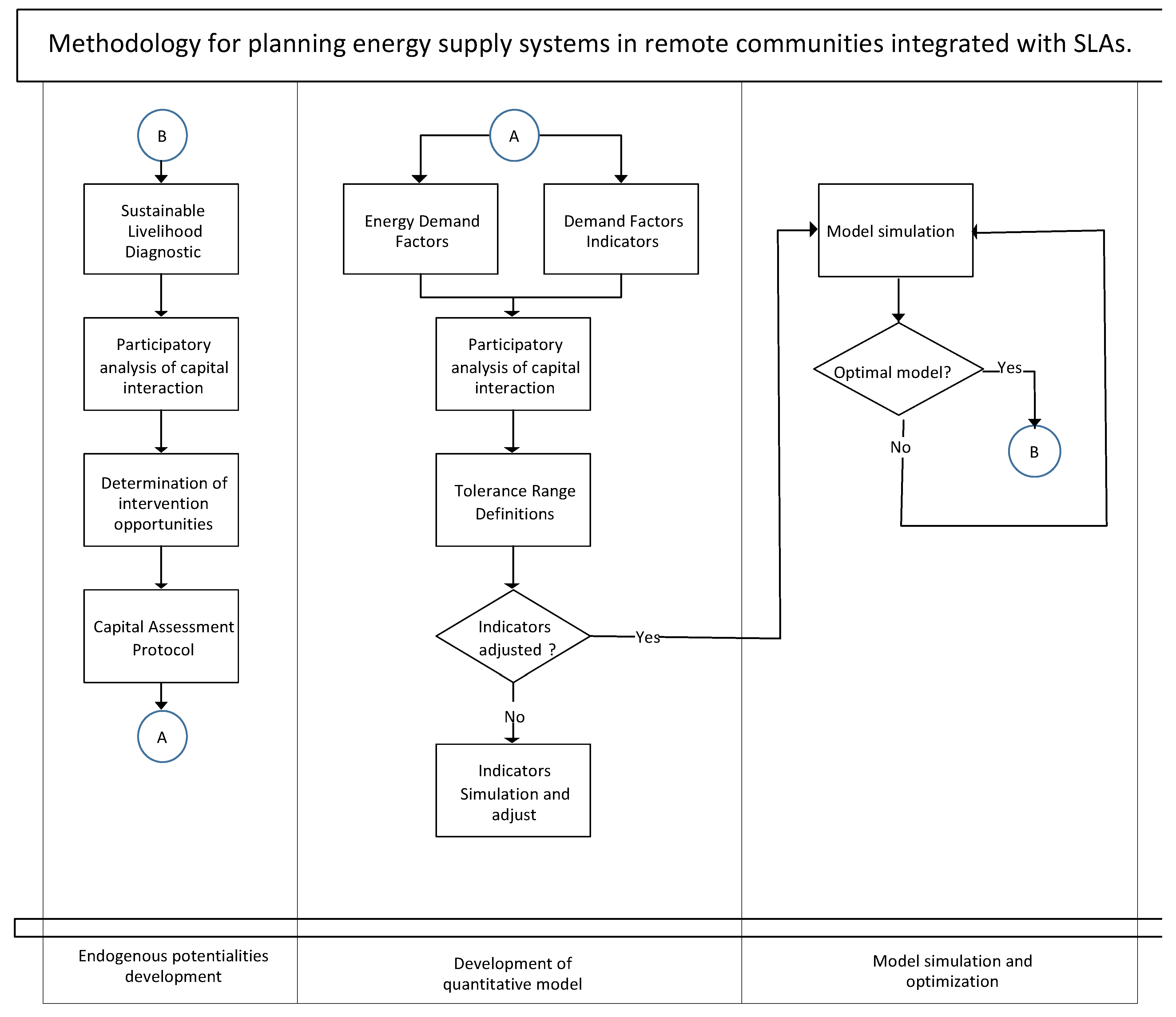
- A methodology that allows guiding decision-making for the development and evolution of the energy supply system in the long term for remote communities.
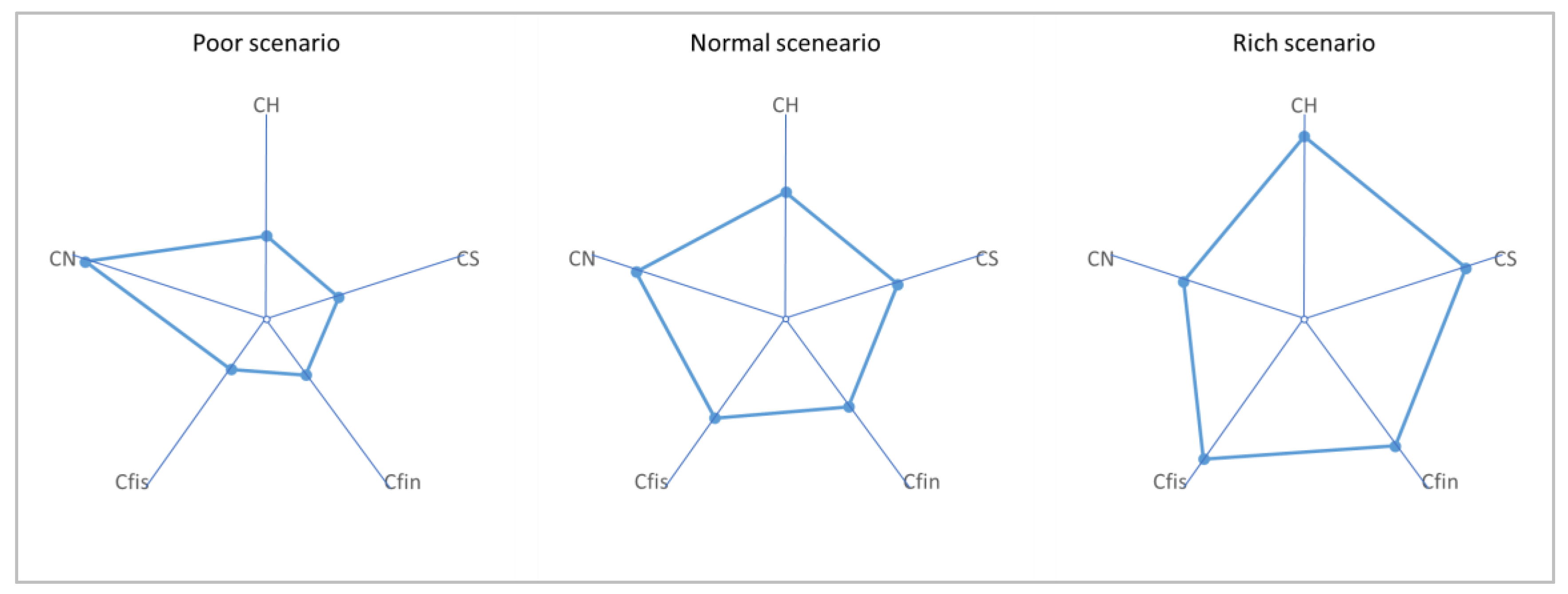
- A process of optimization of the indicators that make up the capitals of the community, taking them from a poor scenario to a rich one as a result and guaranteeing harmonious and sustainable growth between the capitals.
- The integration of long-term energy planning variables and SLs.
2. Systematic Literature Review
2.1. Sustainable Livelihoods Approach
- -
- Human Capital: characterized among others by the levels of health, nutrition, education, and knowledge.
- -
- Social Capital: they are networks and connections between individuals with shared interests, forms of social participation, and relationships of trust and reciprocity.
- -
- Natural Capital: these are the natural resources useful in terms of livelihood.
- -
- Physical Capital: these are the infrastructures and equipment that respond to the basic and productive needs of the population.
- -
- Financial Capital: These are the financial resources that populations use to achieve their livelihood objectives.
2.2. Assets Pentagon
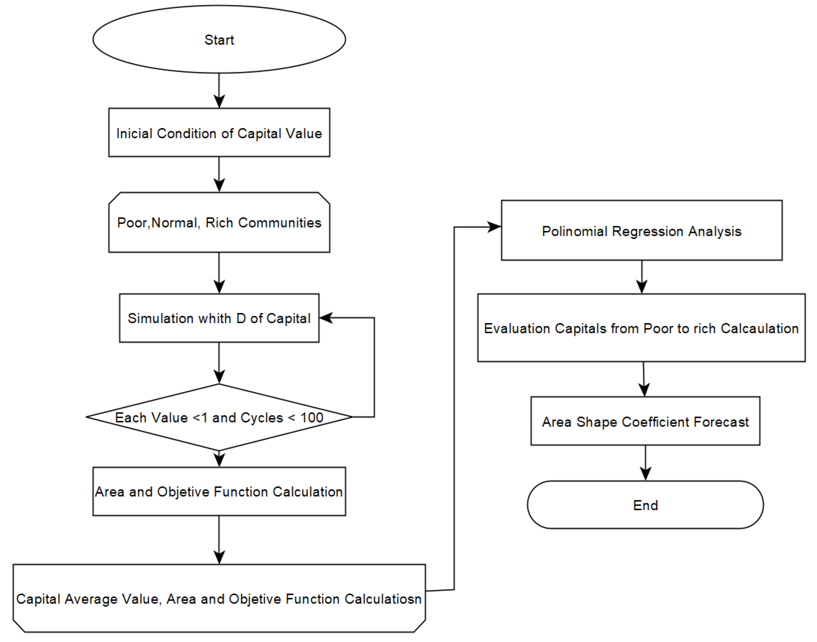
2.3. Simulation Algorithm
2.4. Polynomial Regression
3. Methodology
3.1. Pentagon Area Shape Coefficient
3.2. Capitals Modeling and Simulation Algorithm
4. Results
5. Discussions
6. Conclusions and Recommendations
Author Contributions
Funding
Acknowledgments
Conflicts of Interest
References
- Mustafa Kamal, M.; Asharaf, I.; Fernandez, E. Optimal renewable integrated rural energy planning for sustainable energy development. Sustain. Energy Technol. Assess. 2022, 53, 102581. [Google Scholar] [CrossRef]
- Quevedo, J.; Moya, I.H. Modeling of the dominican republic energy systems with OSeMOSYS to assess alternative scenarios for the expansion of renewable energy sources. Energy Nexus 2022, 6, 100075. [Google Scholar] [CrossRef]
- Pereyra-Mariñez, C.; Santos-García, F.; Ocaña-Guevara, V.S.; Vallejo-Díaz, A. Energy Supply System Modeling Tools Integrating Sustainable Livelihoods Approach—Contribution to Sustainable Development in Remote Communities: A Review. Energies 2022, 15, 2668. [Google Scholar] [CrossRef]
- Castaño-Rosa, R.; Solís-Guzmán, J.; Marrero-Meléndez, M. Midiendo la pobreza energética. Una revisión de indicadores. Rev. Hábitat Sustentable 2020, 10, 08–21. [Google Scholar] [CrossRef]
- Cruz-De-Jesús, E.; Martínez-Ramos, J.L.; Marano-Marcolini, A. Optimal Scheduling of Controllable Resources in Energy Communities: An Overview of the Optimization Approaches. Energies 2022, 16, 101. [Google Scholar] [CrossRef]
- CNE. Analisis Pobreza Energetica Republica Dominicana. Comisión Nacional de Energía. September 2014. Available online: https://www.cne.gob.do/wp-content/uploads/2016/04/analisis-pobreza-energetica-republica-dominicana.pdf (accessed on 2 January 2023).
- Mohsin, M.; Taghizadeh-Hesary, F.; Shahbaz, M. Nexus between financial development and energy poverty in Latin America. Energy Policy 2022, 165, 112925. [Google Scholar] [CrossRef]
- Bhattacharyya, S.C. Review of alternative methodologies for analysing off-grid electricity supply. Renew. Sustain. Energy Rev. 2012, 16, 677–694. [Google Scholar] [CrossRef]
- Calvo, R.; Álamos, N.; Billi, M.; Urquiza, A.; Lisperguer, R.C. Desarrollo de Indicadores de Pobreza Energética en América Latina y el Caribe; CEPAL: Santiago, Chile, 2021. [Google Scholar]
- Liu, Y.; Yu, S.; Zhu, Y.; Wang, D.; Liu, J. Modeling, planning, application and management of energy systems for isolated areas: A review. Renew. Sustain. Energy Rev. 2018, 82, 460–470. [Google Scholar] [CrossRef]
- Montoya-Duque, L.; Arango-Aramburo, S.; Arias-Gaviria, J. Simulating the effect of the Pay-as-you-go scheme for solar energy diffusion in Colombian off-grid regions. Energy 2022, 244, 123197. [Google Scholar] [CrossRef]
- Gutiérrez-Montes, I.A.; de Imbach, P.B.; Ramírez, F.; Payes, J.L.; Say, E.; Banegas, K. MAP-CATIE Las Escuelas de Campo Del; Centro Agronómico Tropical de Investigación y Enseñanza (CATIE): Turrialba, Costa Rica, 2012; p. 67. [Google Scholar]
- Vallejo-Díaz, A.; Herrera-Moya, I.; Fernández-Bonilla, A.; Pereyra-Mariñez, C. Wind energy potential assessment of selected locations at two major cities in the Dominican Republic, toward energy matrix decarbonization, with resilience approach. Therm. Sci. Eng. Prog. 2022, 32, 101313. [Google Scholar] [CrossRef]
- Garabitos Lara, E.; Vallejo Díaz, A.; Ocaña Guevara, V.S.; Santos García, F. Tecno-economic evaluation of residential PV systems under a tiered rate and net metering program in the Dominican Republic. Energy Sustain. Dev. 2023, 72, 42–57. [Google Scholar] [CrossRef]
- Mulenga, E.; Kabanshi, A.; Mupeta, H.; Ndiaye, M.; Nyirenda, E.; Mulenga, K. Techno-economic analysis of off-grid PV-Diesel power generation system for rural electrification: A case study of Chilubi district in Zambia. Renew. Energy 2023, 203, 601–611. [Google Scholar] [CrossRef]
- Akinyele, D.; Belikov, J.; Levron, Y. Challenges of Microgrids in Remote Communities: A STEEP Model Application. Energies 2018, 11, 432. [Google Scholar] [CrossRef] [Green Version]
- FAO M|Guide for Monitoring and Evaluating Land Administration Programs|Organización de las Naciones Unidas para la Alimentación y la Agricultura. Available online: http://www.fao.org/in-action/herramienta-administracion-tierras/glossary/m/es/ (accessed on 4 April 2020).
- Barman, M.; Mahapatra, S.; Palit, D.; Chaudhury, M.K. Performance and impact evaluation of solar home lighting systems on the rural livelihood in Assam, India. Energy Sustain. Dev. 2017, 38, 10–20. [Google Scholar] [CrossRef]
- Chen, H.; Zhu, T.; Krott, M.; Calvo, J.F.; Ganesh, S.P.; Makoto, I. Measurement and evaluation of livelihood assets in sustainable forest commons governance. Land Use Policy 2013, 30, 908–914. [Google Scholar] [CrossRef]
- Fang, Y.; Fan, J.; Shen, M.; Song, M. Sensitivity of livelihood strategy to livelihood capital in mountain areas: Empirical analysis based on different settlements in the upper reaches of the Minjiang River, China. Ecol. Indic. 2014, 38, 225–235. [Google Scholar] [CrossRef]
- DFID. Hojas Orientativas Sobre Los Medios De Vida Sostenibles; DFID: London, UK, 2001; p. 210. [Google Scholar]
- DFID. Sustainable Livelihoods Guidance Sheets; DFID: London, UK, 1999. [Google Scholar]
- Weisstein, E.W.; Polygon Area. From MathWorld—A Wolfram Web Resource. 2022. Available online: https://mathworld.wolfram.com/PolygonArea.html (accessed on 27 November 2022).
- Rahmawati, D.; Rachmawati, T.A.; Prayitno, G. Disaster risk reduction of Mount Kelud eruption based on capacity building: A case study in Kasembon District, Malang Regency. Sustinere J. Environ. Sustain. 2018, 2, 24–42. [Google Scholar] [CrossRef] [Green Version]
- Montgomery, D.C.; Runger, G.C. Applied Statistics and Probability for Engineers; John Wiley & Sons: New York, NY, USA, 2013; ISBN 978-1-118-53971-2. [Google Scholar]
- Jiang, E.; Wang, L.; Peng, Z. Solving energy-efficient distributed job shop scheduling via multi-objective evolutionary algorithm with decomposition. Swarm Evol. Comput. 2020, 58, 100745. [Google Scholar] [CrossRef]
- Wang, G.; Chao, Y.; Cao, Y.; Jiang, T.; Han, W.; Chen, Z. A comprehensive review of research works based on evolutionary game theory for sustainable energy development. Energy Rep. 2022, 8, 114–136. [Google Scholar] [CrossRef]
- Huang, X.; Xia, F.; Xia, Z.; Cong, P.; Di, Z.; Yang, Z.; Song, L. Dynamic Economic Optimal Dispatch of Microgrid Based on Improved Differential Evolution Algorithm. IOP Conf. Ser. Earth Environ. Sci. 2018, 170, 042143. [Google Scholar] [CrossRef] [Green Version]
- Khalid, O.W.; Isa, N.A.M.; Mat Sakim, H.A. Emperor penguin optimizer: A comprehensive review based on state-of-the-art meta-heuristic algorithms. Alex. Eng. J. 2023, 63, 487–526. [Google Scholar] [CrossRef]
- Briones, L.; Escola, J.M. Application of the Microsoft Excel Solver tool in the solution of optimization problems of heat exchanger network systems. Educ. Chem. Eng. 2019, 26, 41–47. [Google Scholar] [CrossRef]
- Outram, J.G.; Couperthwaite, S.J.; Martens, W.; Millar, G.J. Application of non-linear regression analysis and statistical testing to equilibrium isotherms: Building an Excel template and interpretation. Sep. Purif. Technol. 2021, 258, 118005. [Google Scholar] [CrossRef]
- Aldeni, M.; Wagaman, J.; Alzaghal, A.; Al-Aqtash, R. Simultaneous estimation of log-normal coefficients of variation: Shrinkage and pretest strategies. MethodsX 2023, 10, 101939. [Google Scholar] [CrossRef] [PubMed]
- Long, X.; Wu, S.; Wang, J.; Wu, P.; Wang, Z. Urban water environment carrying capacity based on VPOSR-coefficient of variation-grey correlation model: A case of Beijing, China. Ecol. Indic. 2022, 138, 108863. [Google Scholar] [CrossRef]
- Zhao, Y.; Yang, M.; Peng, X.; Li, G. Research on SMEs’ Credit Risk Evaluation Index System from the Perspective of Supply Chain Finance—R-cluster and coefficient of variation based on panel data. Procedia Comput. Sci. 2022, 214, 613–620. [Google Scholar] [CrossRef]
- Mukisa, N.; Zamora, R.; Lie, T.T. Assessment of community sustainable livelihoods capitals for the implementation of alternative energy technologies in Uganda—Africa. Renew. Energy 2020, 160, 886–902. [Google Scholar] [CrossRef]
- Henao, F.; Cherni, J.A.; Jaramillo, P.; Dyner, I. A multicriteria approach to sustainable energy supply for the rural poor. Eur. J. Oper. Res. 2012, 218, 801–809. [Google Scholar] [CrossRef]
- Bhattarai, P.R.; Thompson, S. Optimizing an off-grid electrical system in Brochet, Manitoba, Canada. Renew. Sustain. Energy Rev. 2016, 53, 709–719. [Google Scholar] [CrossRef] [Green Version]
- Martinkus, N.; Rijkhoff, S.A.; Hoard, S.A.; Shi, W.; Smith, P.; Gaffney, M.; Wolcott, M. Biorefinery site selection using a stepwise biogeophysical and social analysis approach. Biomass Bioenergy 2017, 97, 139–148. [Google Scholar] [CrossRef] [Green Version]
- Nadimi, R.; Tokimatsu, K. Potential energy saving via overall efficiency relying on quality of life. Appl. Energy 2019, 233–234, 283–299. [Google Scholar] [CrossRef]
- Yadav, P.; Malakar, Y.; Davies, P.J. Multi-scalar energy transitions in rural households: Distributed photovoltaics as a circuit breaker to the energy poverty cycle in India. Energy Res. Soc. Sci. 2019, 48, 1–12. [Google Scholar] [CrossRef]
- Mahmud, K.; Amin, U.; Hossain, M.J.; Ravishankar, J. Computational tools for design, analysis, and management of residential energy systems. Appl. Energy 2018, 221, 535–556. [Google Scholar] [CrossRef]
- Chinmoy, L.; Iniyan, S.; Goic, R. Modeling wind power investments, policies and social benefits for deregulated electricity market—A review. Appl. Energy 2019, 242, 364–377. [Google Scholar] [CrossRef]
- Khanna, R.A.; Li, Y.; Mhaisalkar, S.; Kumar, M.; Liang, L.J. Comprehensive energy poverty index: Measuring energy poverty and identifying micro-level solutions in South and Southeast Asia Energy Policy 2019, 132, 379–391. Energy Policy 2019, 132, 379–391. [Google Scholar] [CrossRef]
- Søraa, R.A.; Anfinsen, M.; Foulds, C.; Korsnes, M.; Lagesen, V.; Robison, R.; Ryghaug, M. Diversifying diversity: Inclusive engagement, intersectionality, and gender identity in a European Social Sciences and Humanities Energy research project. Energy Res. Soc. Sci. 2020, 62, 101380. [Google Scholar] [CrossRef]
- Karthik, N.; Parvathy, A.K.; Arul, R. A review of optimal operation of microgrids. IJECE 2019, 14, 9. [Google Scholar] [CrossRef]
- Viteri, J.P.; Henao, F.; Cherni, J.; Dyner, I. Optimizing the insertion of renewable energy in the off-grid regions of Colombia. J. Clean. Prod. 2019, 235, 535–548. [Google Scholar] [CrossRef]
- Musonye, X.S.; Davíósdóttir, B.; Kristjánsson, R.; Ásgeirsson, E.I.; Stefánsson, H. Integrated energy systems’ modeling studies for sub-Saharan Africa: A scoping review. Renew. Sustain. Energy Rev. 2020, 128, 109915. [Google Scholar] [CrossRef]
- Lozano, L.; Taboada, E.B. Demystifying the authentic attributes of electricity-poor populations: The electrification landscape of rural off-grid island communities in the Philippines. Energy Policy 2020, 145, 111715. [Google Scholar] [CrossRef]
- Campos, I.; Marín-González, E. People in transitions: Energy citizenship, prosumerism and social movements in Europe. Energy Res. Soc. Sci. 2020, 69, 101718. [Google Scholar] [CrossRef]
- Ahmadi, S.E.; Rezaei, N. A new isolated renewable based multi microgrid optimal energy management system considering uncertainty and demand response. Int. J. Electr. Power Energy Syst. 2020, 118, 105760. [Google Scholar] [CrossRef]


| Capitals and Indicators | Acronym | WB | DFID | UNDP | Total |
|---|---|---|---|---|---|
| Human capital | CH | 1 | 3 | 4 | |
| The economically active population (%) | CHI1 | 1 | 1 | ||
| Occupancy rate | CHI2 | 1 | 1 | ||
| Scholarship | CHI3 | 1 | 1 | ||
| Life expectancy | CHI4 | 1 | 1 | ||
| Family size (According to Organization for Economic Cooperation and Development (OECD).) | CHI5 | ||||
| Labor productivity (According to Organization for Economic Cooperation and Development (OECD).) | CHI6 | ||||
| Social capital | CS | 4 | 1 | 5 | |
| Community Participation Level | CSI1 | 1 | 1 | ||
| Collective representation | CSI2 | 1 | 1 | ||
| Leadership | CSI3 | 1 | 1 | ||
| Participation in decision-making | CSI4 | 1 | 1 | ||
| Climate information services | CSI5 | 1 | 1 | ||
| Financial capital | CF | 8 | 1 | 9 | |
| Local GDP/hab (is taken from the International Monetary Fund (IMF).) | CFI1 | ||||
| Access to credit | CFI2 | 1 | 1 | ||
| Household income | CFI3 | 1 | 1 | ||
| Social help | CFI4 | 1 | 1 | ||
| Arrival of tourists | CFI5 | 1 | 1 | ||
| Grid electricity cost | CFI6 | 1 | 1 | ||
| Spending on energy sources | CFI7 | 1 | 1 | ||
| Remittances | CFI8 | 1 | 1 | ||
| Investment Capital | CFI9 | 1 | 1 | ||
| Savings | CFI10 | 1 | 1 | ||
| Physical capital | CP | 7 | 1 | 2 | 10 |
| Access to information | CPI1 | 1 | 1 | ||
| Access to energy | CPI2 | 1 | 1 | ||
| Energy consumption per inhabitant | CPI3 | 1 | 1 | ||
| Self-coverage of the Energy Demand | CPI4 | 1 | 1 | ||
| Use of renewable energies | CPI5 | 1 | 1 | ||
| Transport infrastructure | CPI6 | 1 | 1 | ||
| Carrier penetration Renewable energy | CPI7 | 1 | 1 | ||
| Grid reliability | CPI8 | 1 | 1 | ||
| Proximity to the grid of the community interconnected system | CPI9 | 1 | 1 | ||
| Access to water | CPI10 | 1 | 1 | ||
| Natural capital | CN | 1 | 7 | 8 | |
| Disponibility of Renewable Energy carriers | CNI1 | 1 | 1 | ||
| Air quality | CNI2 | 1 | 1 | ||
| Particles total | CNI3 | 1 | 1 | ||
| Net absorption CO2 | CNI4 | ||||
| Available Water | CNI5 | 1 | 1 | ||
| Biodiversity | CNI6 | 1 | 1 | ||
| Forest cover area | CNI7 | 1 | 1 | ||
| Hydrographic basin management | CNI8 | 1 | 1 | ||
| Availability of water and aquatic resources | CNI9 | 1 | 1 | ||
| Total | 17 | 6 | 13 | 36 | |
| Capitals and Indicators | Acronym | WB | DFID | UNDP | Total |
| Human capital | CH | 1 | 3 | 4 | |
| The economically active population (%) | CHI1 | 1 | 1 | ||
| Occupancy rate | CHI2 | 1 | 1 | ||
| Scholarship | CHI3 | 1 | 1 | ||
| Life expectancy | CHI4 | 1 | 1 | ||
| Family size (According to Organization for Economic Cooperation and Development (OECD).) | CHI5 | ||||
| Labor productivity (According to Organization for Economic Cooperation and Development (OECD).) | CHI6 | ||||
| Social capital | CS | 4 | 1 | 5 | |
| Community Participation Level | CSI1 | 1 | 1 | ||
| Collective representation | CSI2 | 1 | 1 | ||
| Leadership | CSI3 | 1 | 1 | ||
| Participation in decision-making | CSI4 | 1 | 1 | ||
| Climate information services | CSI5 | 1 | 1 | ||
| Financial capital | CF | 8 | 1 | 9 | |
| Local GDP/hab (is taken from the International Monetary Fund (IMF).) | CFI1 | ||||
| Access to credit | CFI2 | 1 | 1 | ||
| Household income | CFI3 | 1 | 1 | ||
| Social help | CFI4 | 1 | 1 | ||
| Arrival of tourists | CFI5 | 1 | 1 | ||
| Grid electricity cost | CFI6 | 1 | 1 | ||
| Spending on energy sources | CFI7 | 1 | 1 | ||
| Remittances | CFI8 | 1 | 1 | ||
| Investment Capital | CFI9 | 1 | 1 | ||
| Savings | CFI10 | 1 | 1 | ||
| Physical capital | CP | 7 | 1 | 2 | 10 |
| Access to information | CPI1 | 1 | 1 | ||
| Access to energy | CPI2 | 1 | 1 | ||
| Energy consumption per inhabitant | CPI3 | 1 | 1 | ||
| Self-coverage of the Energy Demand | CPI4 | 1 | 1 | ||
| Use of renewable energies | CPI5 | 1 | 1 | ||
| Transport infrastructure | CPI6 | 1 | 1 | ||
| Carrier penetration Renewable energy | CPI7 | 1 | 1 | ||
| Grid reliability | CPI8 | 1 | 1 | ||
| Proximity to the grid of the community interconnected system | CPI9 | 1 | 1 | ||
| Access to water | CPI10 | 1 | 1 | ||
| Natural capital | CN | 1 | 7 | 8 | |
| Disponibility of Renewable Energy carriers | CNI1 | 1 | 1 | ||
| Air quality | CNI2 | 1 | 1 | ||
| Particles total | CNI3 | 1 | 1 | ||
| Net absorption CO2 | CNI4 | ||||
| Available Water | CNI5 | 1 | 1 | ||
| Biodiversity | CNI6 | 1 | 1 | ||
| Forest cover area | CNI7 | 1 | 1 | ||
| Hydrographic basin management | CNI8 | 1 | 1 | ||
| Availability of water and aquatic resources | CNI9 | 1 | 1 | ||
| Total | 17 | 6 | 13 | 36 |
| Variable | Description | Value |
|---|---|---|
| xCh | Component x of Human Capital | 0 |
| xCs | Component x of Social Capital | |
| xCfin | Component x of Financial Capital | |
| xCfis | Component x of Physical Capital | |
| xCn | Component x of Natural Capital | |
| yCh | Component and Human Capital | |
| yCs | Component of Social Capital | |
| yCfin | Component y of Financial Capital | |
| yCfis | Component y of Physical Capital | |
| yCn | Component y of Natural Capital |
| Capitals | Equations |
|---|---|
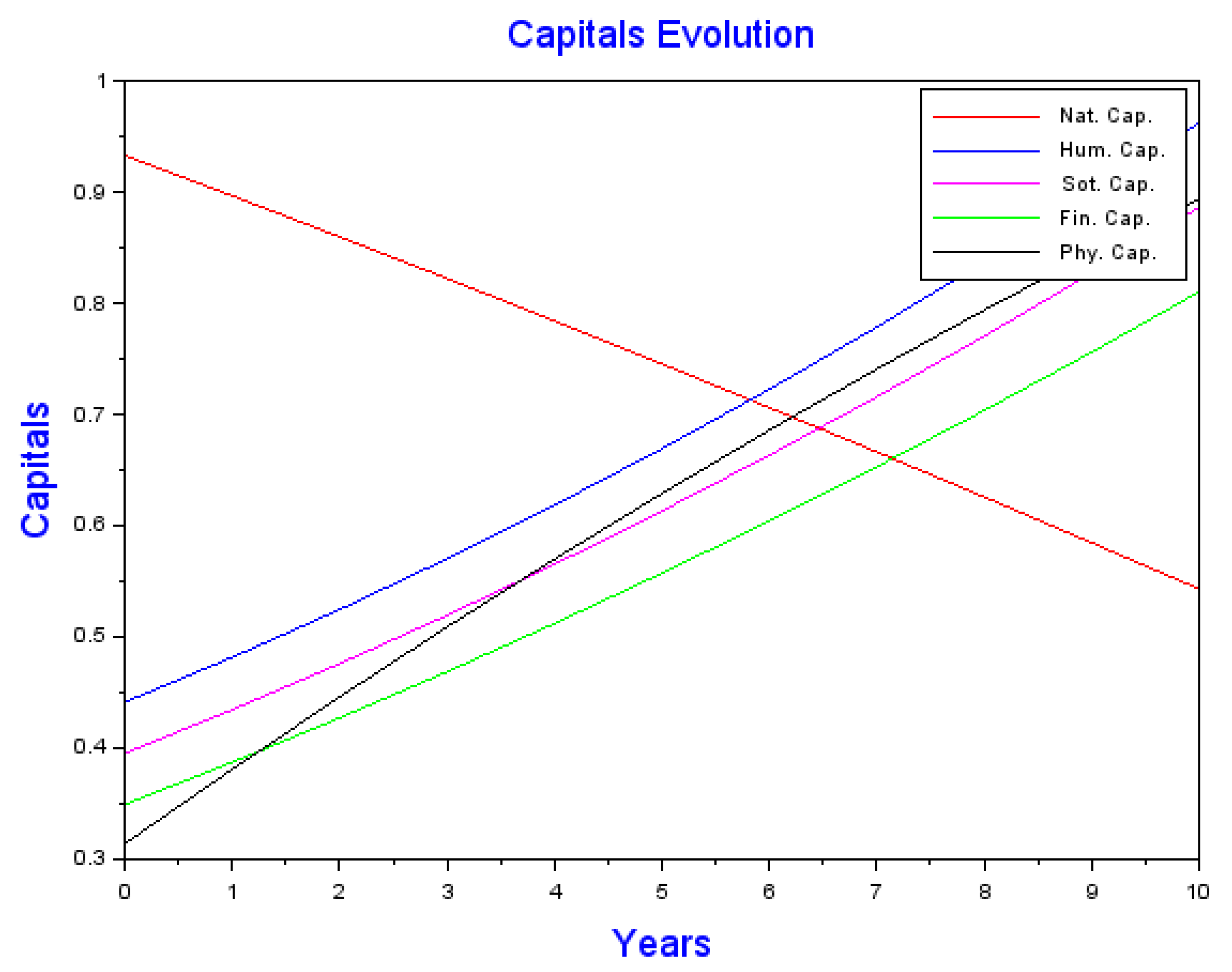
| Human capital | y = 0.0013x2 + 0.0391x + 0.4412 |
| Social capital | y = 0.0011x2 + 0.0381x + 0.3952 |
| Financial capital | y = 0.0009x2 + 0.0371x + 0.3492 |
| physical capital | y = −0.001x2 − 0.068x + 0.3139 |
| natural capital | y = −0.0003x2 − 0.036x + 0.9933 |
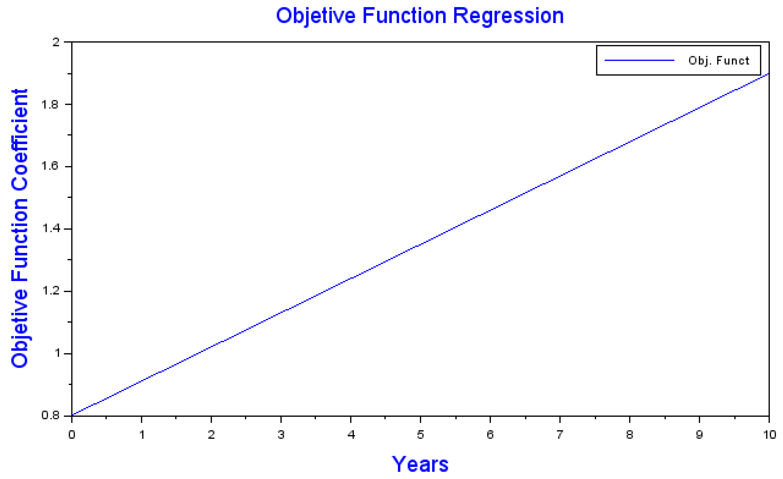
| Period | Objective Function | |||||
|---|---|---|---|---|---|---|
| 0 | 0.4412 | 0.3952 | 0.3492 | 0.3139 | 0.9933 | 0.80 |
| 1 | 0.4816 | 0.4344 | 0.3871 | 0.3809 | 0.9576 | 0.91 |
| 2 | 0.5246 | 0.4758 | 0.4268 | 0.4459 | 0.9225 | 1.02 |
| 3 | 0.5702 | 0.5194 | 0.4683 | 0.5089 | 0.8880 | 1.13 |
| 4 | 0.6184 | 0.5652 | 0.5116 | 0.5699 | 0.8541 | 1.24 |
| 5 | 0.6692 | 0.6132 | 0.5567 | 0.6289 | 0.8208 | 1.35 |
| 6 | 0.7226 | 0.6634 | 0.6036 | 0.6859 | 0.7881 | 1.46 |
| 7 | 0.7786 | 0.7158 | 0.6523 | 0.7409 | 0.7560 | 1.57 |
| 8 | 0.8372 | 0.7704 | 0.7028 | 0.7939 | 0.7245 | 1.68 |
| 9 | 0.8984 | 0.8272 | 0.7551 | 0.8449 | 0.6936 | 1.79 |
| 10 | 0.9622 | 0.8862 | 0.8092 | 0.8939 | 0.6633 | 1.90 |
| No. | References | SLA | Optimized Model | Capitals, Indicators and Variables Projected | Temporal Resolution | Spatial Resolution |
|---|---|---|---|---|---|---|
| 1 | Proposed Model | YES | YES | YES | Long Term | Local |
| 2 | Henao [36] | YES | NO | NO | Specific conditions | Local |
| 3 | Bhattarai and Thompson [37] | - | NO | NO | Specific conditions | Local |
| 4 | Martinkus [38] | YES | NO | NO | Specific conditions | Local |
| 5 | Huang et al. [28] | - | NO | NO | Long-term | Regional |
| 6 | Nadimi and Tokimatsu [39] | - | NO | NO | Long-term | Global |
| 7 | Yadav et al. [40] | - | NO | NO | Long-term | Global |
| 8 | Mahmud et al. [41] | - | NO | NO | Long-term | Global |
| 9 | Akinyele et al. [16] | - | NO | NO | Specific conditions | Local |
| 10 | Chinmoy et al. [42] | - | NO | NO | Long-term | Global |
| 11 | Khanna et al. [43] | - | NO | NO | Long-term | Regional |
| 12 | Søraa et al. [44] | - | NO | NO | Long-term | Global |
| 13 | Karthik et al. [45] | - | NO | NO | Specific conditions | Local |
| 14 | Viteri et al. [46] | - | NO | NO | Specific conditions | Regional |
| 15 | Mukisa et al. [35] | YES | YES | NO | Specific conditions | Local |
| 16 | Musonye et al. [47] | - | NO | NO | Long-term | Global |
| 17 | Lozano and Taboada [48] | - | NO | NO | Long-term | Global |
| 18 | Campos and Marín-González [49] | - | NO | NO | Long-term | Global |
| 19 | Ahmadi & Rezaei [50] | - | NO | NO | Specific conditions | Local |
Disclaimer/Publisher’s Note: The statements, opinions and data contained in all publications are solely those of the individual author(s) and contributor(s) and not of MDPI and/or the editor(s). MDPI and/or the editor(s) disclaim responsibility for any injury to people or property resulting from any ideas, methods, instructions or products referred to in the content. |
© 2023 by the authors. Licensee MDPI, Basel, Switzerland. This article is an open access article distributed under the terms and conditions of the Creative Commons Attribution (CC BY) license (https://creativecommons.org/licenses/by/4.0/).
Share and Cite
Pereyra-Mariñez, C.; Andrickson-Mora, J.; Ocaña-Guevera, V.S.; Santos García, F.; Vallejo Diaz, A. Energy Supply Systems Predicting Model for the Integration of Long-Term Energy Planning Variables with Sustainable Livelihoods Approach in Remote Communities. Energies 2023, 16, 3143. https://doi.org/10.3390/en16073143
Pereyra-Mariñez C, Andrickson-Mora J, Ocaña-Guevera VS, Santos García F, Vallejo Diaz A. Energy Supply Systems Predicting Model for the Integration of Long-Term Energy Planning Variables with Sustainable Livelihoods Approach in Remote Communities. Energies. 2023; 16(7):3143. https://doi.org/10.3390/en16073143
Chicago/Turabian StylePereyra-Mariñez, Carlos, José Andrickson-Mora, Victor Samuel Ocaña-Guevera, Félix Santos García, and Alexander Vallejo Diaz. 2023. "Energy Supply Systems Predicting Model for the Integration of Long-Term Energy Planning Variables with Sustainable Livelihoods Approach in Remote Communities" Energies 16, no. 7: 3143. https://doi.org/10.3390/en16073143
APA StylePereyra-Mariñez, C., Andrickson-Mora, J., Ocaña-Guevera, V. S., Santos García, F., & Vallejo Diaz, A. (2023). Energy Supply Systems Predicting Model for the Integration of Long-Term Energy Planning Variables with Sustainable Livelihoods Approach in Remote Communities. Energies, 16(7), 3143. https://doi.org/10.3390/en16073143