Article

Analysis of the Thermo-Aeraulic Behavior of a Heated Supply Air Window in Forced Convection: Numerical and Experimental Approaches

Univ. Artois, IMT Nord Europe, Junia, Univ. Lille, ULR 4515, Laboratoire de Génie Civil et géo-Environnement (LGCgE), F-62400 Béthune, France
*
Author to whom correspondence should be addressed.
Energies 2023, 16(7), 3243; https://doi.org/10.3390/en16073243
Submission received: 28 February 2023 / Revised: 24 March 2023 / Accepted: 29 March 2023 / Published: 4 April 2023

Abstract

:
This paper presents work intended to characterize air flow and convective heat transfers within a ventilated window. This window is a device that allows for the entry of fresh air into a building while simultaneously preheating it in order to satisfy requirements in terms of air quality and thermal comfort in inhabited spaces. Therefore, this essential component of the building envelope functions herein as a heat exchanger with its own geometric characteristics and exchange conditions. In this research, a dual numerical and experimental approach has been implemented in order to highlight the temperatures, velocities and heat flux fields both at the glazing surfaces and in the ventilated air gaps. Several turbulence models were tested using CFD software (ANSYS-FLUENT®); their results were compared with each other as well as with the experimental results. This study shows that the air gap geometry in the window induces flow disturbances, recirculation phenomena and non-uniform heat exchanges, all of which prove to be important in terms of overall component performance. With regard to modeling and, in particular, at the level of turbulence models, the results obtained indicate that the model GEKO is best suited to the configuration under study when the phenomena of turbulent forced convection dominate the dynamics of the transfers. The k-ε models reveal a tremendous weakness in precisely estimating the problem’s characteristic quantities. From an experimental point of view, local measurements of thermal fluxes and temperatures demonstrate high efficiency with regard to experimental technique, which in turn could be extended to many different configurations for the local evaluation of convection heat transfer.

1. Introduction

The envelope is the main element to be taken into consideration when constructing a building with low energy consumption; it is the interface between indoor and outdoor environments and the basis of heat and mass transfers. If this envelope performs well, then the mechanical equipment for heating and cooling becomes secondary. The energy transition, which has become essential, coupled with the need to minimize climate change is driving successive modifications in thermal regulations, imposing reductions in a building’s energy consumption by focusing on both thermal insulation and the airtightness of the walls. For several years, particularly in the case of a building’s renovation, it has been found that these developments can at times lead to disorders. However, ventilation is essential for occupants’ health and comfort as well as for the preservation of a building’s durability.
Among the studies carried out in the past on the so-called “classical” parietodynamic window, Powell [1], Boehm [2], et Korkala [3] and Paziaud [4] deserve mention. In general, these authors have highlighted the key role played by the parietodynamic window in reducing building energy consumption.
This work is tied to the European research project entitled ‘VARIETO’, where the name refers to combined heated and ventilated windows; it is being funded by ADEME (France’s Agency for the Environment and Energy Management). It consists of analyzing the behavior and performance of a ventilated heating window system. The window is a Paziaud variant [4] (Figure 1a) of the parietodynamic window; it has been designed to contribute simultaneously to heating, ventilation and natural lighting inside a building. The underlying operating principle is to force the fresh air to circulate within a U-shaped channel formed by three panes of glass.
Hence, in winter, energy loss from the building is recovered in order to preheat fresh air before it enters the room. During daytime, the window also allows for the recovery of solar radiation absorbed by the glazing. In the present study, one of the three glazed panes is being heated. The window thus acts as a heat emitter.
In recent years, studies conducted by Gloriant and Greffet [5,6] have led to significant advances in the industrialization of these windows and the integration of this component into thermal building regulations. The “ventilated heating window” configuration is one variant under study in this article.
In the context of energy and climate change, many types of “active” facades are being studied given the increasing importance of this topic. A bibliographic review [7] was carried out on “multi-skin” ventilated facades and it highlighted the significant gains that could be obtained in overall building energy balance. Investigations have been performed to study the various types of ventilated windows, such as the simple pivoting window [8], the ventilated double-glazing window [9] (Figure 1b) and the double-skin window [10] (Figure 1c). This research demonstrates the major effects of such windows in reducing cooling loads in summer and heating loads in winter while providing fresh air to building occupants through mechanical or naturally assisted ventilation. All these studies have underscored the importance of improving building envelope quality, in particular airtightness, in order to optimize airflow in ventilated “walls” and thus contribute to reducing the energy consumption of healthier and greener buildings as part of the global strategy to reduce carbon emissions [11,12].
Several construction and environmental parameters serve to influence the thermal behavior of windows; these parameters need to be studied in greater detail. In particular, the present research focuses on how thermal energy is recovered and transferred by components. As with any heat exchanger, flow rates and geometric characteristics will influence the airflow passing through the ventilated channel. Three distinct modes of operation can be considered: forced, natural, or mixed ventilation. Natural ventilation occurs through two mechanisms, i.e., a driving force generated by the temperature difference between the outer space and the ventilated channel and a pressure differential related to the effects of wind on the facade. Forced ventilation is only used when the driving forces providing natural ventilation become insufficient to obtain the required performance. Forced ventilation also offers the advantage of easily controlling fresh air flow rates by adjusting them to satisfy needs using a regulating device. In the case of a heating window, the two principles (natural and forced convection) are superimposed in proportions that vary according to the use conditions.
Gloriant et al. [13] were interested in studying the ventilated window with triple glazing in terms of thermal performance without taking solar radiation into account. In order to carefully explore the heat transfers taking place both inside and outside the window, a large number of sensors (thermocouples, heat flux meters, etc.) were implemented. As a result, heat exchange coefficients were evaluated locally, which contributed to developing a validated 2D model for the experimental configuration. Nevertheless, several zones in the cavities remained unexplored due to singularities and turbulence phenomena in the flow.
Michaux et al. [14] developed a pseudo-three-dimensional nodal model for a triple-glazed ventilated window. The convective heat transfer coefficients input into the model were derived from the approach proposed by our team and validated by Gloriant [15]. The particularity of this model is that it takes into account lateral heat transfers to the window frame, which enables the refinement of the calculation of the overall window energy balance. In this study, experiments have also made it possible to identify “dead” zones in the air gaps due to the geometry of the air inlet and outlet vents, whose width is smaller than that of the window.
Khalvati and Omidvar [16] proposed a zonal model for a double-glazed ventilated window so as to define the optimal airflow channel and aspect ratio of the window to be used in an evaporatively cooled building, thereby saving energy and improving the thermal comfort of the building’s inhabitants. Wei et al. [17] developed an analogical model to consider two-dimensional heat transfer in a double airflow window system (Figure 1d), then coupled this model to a building in the “EnergyPlusTM” software. Their model was validated using a test cell with a window ventilated under actual weather conditions before being applied to examine the energy performance of a small apartment installed with double-flow windows in five different climate zones across China. The average energy savings rates resulting from the application of airflow were approximately 25% for cold climates and 21% for warm climates [18,19].
More detailed studies have been carried out using computational fluid dynamics (CFD) for mechanically ventilated facades. Raffnsøe [20] compared two numerical models simulating a window with airflow through a U-shaped channel: one based on ISO 15,099 [21], the other CFD-based. The author pointed out that heat flux within the window varies according to the air flow rate as well as its performance.
Southall and McEvoy [22] also explored the operation of a single-gap ventilated window. Their study was validated by both experimentation in a test cell and simulations using ESP-r and CFD. These authors deduced that the phenomena of turbulence in the air gap and at the surface of the glazing are predominant in characterizing the thermal transmission through the window, leading to the deduction of the temperature of blown air. Bhamjee et al. [23] proposed a three-dimensional CFD model for an airflow double-glazed window. These models were validated experimentally; however, the mean error between experiment and CFD equaled 44% for the intensity of turbulence in the cavities, due to flow seeding problems as well as the isotropic turbulence hypothesis inherent in the turbulence model (SST k-ω) employed.
Khosravi et al. [24] conducted a study on a ventilated window in winter mode. The aim herein was to analyze the preheated fresh air passing through the window along with its performance. This work was based on a detailed parametric study. A 3D CFD model using the “K-ε realizable” turbulence model was implemented. The authors compared six configurations of ventilated windows by varying: (1) cavity width; (2) height; (3) inlet window width; and (4) double-glazing location with a closed air plate. They deduced that improved thermal performance could be achieved with a ventilated window with double glazing located on the interior side and a smaller width. In addition, the increase in temperature of the air blown inside depended on the cavity’s dimensions.
In the present work, the Paziaud ventilated window with triple glazing is studied in the form of a variant, whereby the interior glazing is heated. For this project, the component has been the subject of a number of both laboratory and in situ experiments [25]. This article develops a numerical model and proceeds with its validation according to laboratory experiments. In particular, the objective here is to study window operations when the flow is forced and disturbed by the generation of turbulence and then subjected to a thermal entrainment effect linked to the presence of heated glazing. The characteristic flow parameters and heat source effect were evaluated and compared under several configurations. The definition and determination of convective heat transfer coefficients in the heating window, plus the problem of their determination, are also considered.

2. Materials and Methods

2.1. Physical Problems and Experimental Set-Up

2.1.1. Physical Problem

In the ventilated window, air flow is generated by the pressure differential between the air inlet and outlet, i.e., between the internal and external environments. In the case of the heating window, this phenomenon differs slightly due to the presence of an integrated heat source. Let us note that the flow in the window is influenced by many of the parameters that serve to generate the flow, namely:
Thermal pulling: a phenomenon that depends on the temperature difference between indoor and outdoor environments as well as on the solar inputs and power injected into the heating window.
A mechanical device (extractor): a slight depression of between 4 Pa and 30 Pa is generally considered for such a system.
The effects of wind pressure on facades: a study carried out by the STCB organization [26] on a conventional parietodynamic window showed that, for a pressure difference of less than 30 Pa between indoor and outdoor environments, the fact of circulating air between the walls of a window did not generate additional pressure losses compared to a conventional air inlet. Furthermore, tests performed by Paziaud SA in various renovated dwellings equipped with conventional parietodynamic windows revealed that the measured flow rates lie between 8 and 15 m3 h−1 and, moreover, are relatively stable over time when a mechanical ventilation device is present. In this configuration, convection is therefore forced or mixed. Since air velocities remain low in the case of a heated window, complications arise because two fluid entrainment phenomena exist simultaneously. The Richardson Ri number is typically used to determine the influence of gravity effects and the type of convection. If this number is significantly less than one, then the convection is considered to be dynamically unstable and turbulent [27].
This criterion was questioned by Padet [28], who considered that only the thermal buoyancy coefficient Ri.Re is representative of the nature of convection (Re: Reynolds number):
R i . R e = ρ . g . β . T . 2 e 2 μ . V = 14,400 . ρ . g . β . T . e 3 . l μ . Q v
Under a mixed convection mode, the velocity profile is influenced by the temperature difference between the two sides of the heating window. The profile will tend to lean towards the heated side and a counterflow is capable of forming. According to Padet [28], a downward flow occurs near the cold wall when the thermal buoyancy coefficient Re.Ri reaches 288. For a constant air flow, the gravity effects become more pronounced as cavity thickness increases. Indeed, if the Reynolds number remains constant, the increase in cavity thickness “e” is accompanied by a decrease in the velocity “V” in the pipe and a strengthening of gravity effects (i.e., an increase in the Richardson number). In the thermal thrust coefficient, cavity thickness “e” appears with an exponent of three and seems to be the parameter with the greatest influence on the type of convection. If it is being sought to avoid a return flow phenomenon, then it becomes important to maintain a small cavity thickness. In the case of the heating window, flow rates may be higher without risking a cold wall effect, which would cause discomfort. Therefore, the convection is considered herein to be forced; moreover, the velocity profile is assumed to be parabolic at the inlet and symmetrical with respect to the central axis of the cavity. The laminar or turbulent nature of the flow thus depends on the Reynolds number, which varies with air velocity.

2.1.2. Experimental Set-Up

In the context of comparing numerical simulations, experimental data also appear to be essential. Figure 2a,b present the heating window during its instrumentation and integration into the separating wall of two climate cells. The prototype was made of wood and designed for easy glazing removal. The openings for the air inlet and outlet are free rectangular spaces between the top of the interior and exterior glazing and the top of the frame, over the entire width of the window. At the bottom of the window, the air passes under the central pane between two support wedges placed on the sides. These wedges make it possible to hold the central window in place and ensure continuity of the flow in the U-shaped channel thus formed inside the window. It should be noted that these wedges can generate lateral flow disturbances due to a slight narrowing of the air passage. The window is instrumented with T-type thermocouples and heat flux meters (Figure 2a,b). These sensors were placed outside and, more specifically, inside the window along horizontal planes and at several heights. This measurement plan was defined and designed previously for CFD simulations.
The measurements are local yet still allow obtaining a spatial evolution of the various measured quantities (temperatures, fluxes) according to a profile passing through the window thickness at mid-height (see Figure 3b for h = 61 cm).
Five heat flux and temperature sensors were placed along face 5 of the heating glazing (inside the air gap). These sensors were distributed over the height so as to record essential values in three “sensitive” areas in the window (the recirculation zone, the fully developed flow zone and the high thermal gradient zone).
To measure and control airflow through the window, the device installed comprised of the following:
A plenum is placed in front of the window air outlet to ensure good airtightness between the air extraction duct and the window. This instrument avoids disturbances related to the cell environment and, above all else, allows for an accurate measurement of airflow through the window [29];
A ventilation duct connects the plenum to a variable-speed mechanical extractor. This duct was thermally insulated.
The thermocouples used were of the T type (copper/constantan) and allowed local measurement of both the surface temperatures of the glazed walls and the air temperatures. For the low emissive glazing surface (face 3—Figure 3b), a reflective aluminum adhesive was introduced to glue the thermocouples while ensuring extreme cleanliness to limit radiative disturbances. For surfaces without a low-emissivity coating, the thermocouples were mounted on the walls with semi-transparent Kapton adhesive tape. The thermocouples used to measure air temperature were fastened at the center of each cavity by a very thin nylon thread, stretched vertically across the axis of symmetry of the window. Thermocouples were also installed at the window inlet (T100) and outlet (T500), as well as at the junction between the two air gaps at the lower part (T300). This same configuration applied to thermocouple T200 held suspended in the first air gap.
The heat flux sensors used were Captec™ sensors with tangential gradients (Leclercq and Thery) [30,31]. The underlying operating principle is based on the Seebeck thermoelectric effect and relies on a temperature difference, generated in the plane of the sensor, from which a thermal flux measurement can be obtained. Thanks to this principle, the advantage of a reduced thickness (a few tenths of a millimeter) is therefore gained while maintaining high sensitivity (a few tens of microvolts per W/m2). This set-up makes it possible to place heat flux meters in the air gaps without the measurement step becoming too intrusive. Each flux meter has a surface area of 40 cm2 (2 cm × 20 cm); moreover, they are only mounted to those walls without a low emissive coating by means of “spray-on” glue. The integration of the heat flux and temperature sensors was carried out with great precision in order to avoid deformation of the sensors during their insertion into the window. The various heat flux meters were also covered with a matt black paint, thus making it possible to obtain homogeneous emissivity at the sensor surface close to that of glass in infrared radiation as well as to prevent reflections.
The data acquisition step was carried out with a Keithley 2700 multimeter. This device is provided with an IEEE488 interface, enabling computer connectivity. In the present study, an acquisition of all measurements was performed every 30 s for all sensors.

2.2. Numerical Set-Up

This study has focused in particular on when the forced air flow in the window is turbulent and in the steady state, as governed by the equations of fluid mechanics. The thermophysical properties of the fluid are temperature-dependent and calculated according to the recommendations listed in Standard ISO-15099 [21] using polynomial functions. On the external surfaces (Figure 4), linearized Fourier exchange conditions were applied. The conservation equations characterizing this problem will be briefly recalled herein in as much as they are conventional. They were numerically resolved using the Ansys-Fluent© calculation code within a two-dimensional configuration; moreover, they were discretized over the entire grid. The Patankar and Spalding [32] SIMPLE algorithm was used to solve the coupling between pressure and speed. A numerical solution is assumed to converge when the residuals for the various physical quantities become smaller than 10 8 . The independence of this solution with respect to the various meshes was checked to ensure the accuracy of our results. The discrete ordinate radiation (OD) model was used to resolve long-wavelength radiative transfer. It should be noted that for the entire study, solar radiation with short wavelengths was not taken into account.
In order to study the air flow dynamics in the window in greater detail and extend our understanding of the velocity field structure, several numerical tests were carried out on various available turbulence models, which in theory are capable of responding favorably to our needs. An incompressible fluid was assumed in both turbulent flow and steady state. More specifically, these assumptions were made after ascertaining that the Mach number at the channel inlet was less than 0.3. Therefore, for the first family ➀ of tests, the turbulence was modeled using the models: k-ε with standard wall functions: 1-k-ε-Standard so-called (STD), 2-k-ε-RNG “renormalization group” and 3-k-ε-Realizable.
In the second test family ➁ of the turbulence model, k-ε with enhanced wall treatment: 4-k-ε-STD, 5-k-ε-RNG and 6-k-ε-Realizable were used.
Lastly, for the final turbulence model test family ➂, three turbulence models: 7-k-ω-Standard, 8-k-ω-GEKO “Generalized k-ω” and 9-SST-k-ω “Shear-Stress Transport” were tested.
Although the former models of two-equation closures in turbulent flows did show some improvement in result accuracy, they are not best suited to the present configuration (Figure 4). Consequently, a new Generalized k-ω (GEKO) adjustable model was recently proposed by ANSYS Inc. (Canonsburg, PA, USA) to cover a wide range of flow scenarios by providing several freely adjustable parameters. Similarly, changing these physical parameters does not affect the thermal and dynamic behavior of the air flow [33]. Publications on the details of the GEKO model are rather limited [34,35]. The GEKO model offers six free parameters that can be calibrated on the basis of experimental data. In the present case, the default values (CSEP = 1.75, CNW = 0.5, CMIX = CMixCor ≈ 0.30 and CJET = 0.9) were applied, which represent, respectively, the flow separation from smooth walls, the heat transfer for near-wall flows, the free shear flow mix, the corner flow separation and the free jet spreading rates.
The SST model was developed by Menter [36] for a wide range of turbulent flows with fewer variable pressure gradients; hence, modifications were added to take the diffusion term into account in the transport equation. This addition makes it possible to efficiently treat the flow structure as close as possible to the wall.
In the following, a brief recall of the Reynolds-Averaged Navier-Stokes (RANS) in steady state is provided, i.e., the equations for conserving both mass (continuity) and momentum, to which the energy conservation equation was added. The turbulence models used as closure models will also be briefly described here:
Continuity equation:
( ρ U j ) x j = 0
Momentum equations:
x j ( ρ U i U j ) = P x i + x j ( S i j ρ U i U j ¯ )
S i j = μ ( U i x j + U j x i ) 2 3 μ U m x m δ i j
And
ρ u i u j ¯ = μ t U i x j + U j x i 2 3 ρ k + μ t U m x m δ i j
and
μ t = ρ C μ k 2 ε
C µ is a constant.
Turbulent energy transport equation:
x i ( ρ k U i ) = x j ( μ + μ t σ k ) k x j + G k + G b ρ ε
Energy dissipation transport equation:
x i ( ρ ε U i ) = x j ( μ + μ t σ ε ) ε x j + C 1 ε ε k ( G k + C 3 ε G b ) C 2 ε ρ ε 2 k
where C 1 ε , C 2 ε and C 3 ε are constants, σ k , σ ε : turbulent Prandlt numbers for k and ε, respectively, G k : in-line turbulence kinetic energy production for mean velocity gradient, G b : in-line turbulence kinetic energy production for the buoyancy effect.

2.2.1. The Near Wall

The modeling of the phenomena developed in the boundary layers at the walls has a significant impact on the reliability of the numerical solutions obtained. These walls, which serve to limit the flow field, represent one of the main sources of vorticity and turbulence; moreover, these are the zones where the variables of the numerical solution possess a high gradient with respect to momentum and transport. Consequently, the very precise level of flow representation in these regions close to the walls depends on the outcome of the numerical prediction of wall-related turbulence. This study has entailed a sensitivity analysis of the so-called “Standard wall function law” and a second so-called “enhanced wall treatment law”, with the understanding that these two laws were tested using k-ε turbulence models.

2.2.2. Standard Wall Functions

The standard wall function “swf” available in Ansys-Fluent was successfully employed in a large number of industrial flow studies, as proposed by Launder and Spalding [37], who considered constant shear conditions and the equality of kinetic energy production and its dissipation rate in areas close to the wall. Similarly, these authors considered that the mean speed could be evaluated according to a logarithmic law, denoted “log-low”. This evaluation of the mean speed was carried out as a function of the pressure gradient effects in these zones. This particular concept is based on developing the first two layers so as to calculate the turbulent kinetic energy in cells near the wall.

2.2.3. Enhanced Wall Treatment

The wall treatment of the so-called “enhanced”, denoted “ewt”, calls for a method for modeling boundary layers close to the wall based on a two-layer model applicable to a thin mesh in these zones. According to this model, the area close to the wall and affected by fluid viscosity is entirely resolved up to the viscous underlayer. In this approach, the area of zones close to the wall is subdivided into two regions: a region affected by viscosity and an entirely turbulent region. This concept has made it possible to determine the turbulent viscosity in cells close to the wall. Use of this enhanced treatment requires a sufficiently thin mesh to obtain a stable numerical solution [38]. The viscosity-affected region is defined as a function of the local Reynolds number Rey < 200, while the turbulent region is defined when Rey > 200, where “y” is the distance between the nearest wall and the location of the centroid of the cell. The recommended value for an improved treatment of these zones is on the order of y+ ≈ 1.

2.2.4. Heat Transfer

The energy equation adopted for the flow field in the window is given by the following equation [38]:
. ( u ( ρ E + p ) ) = ( k e f f T ) + s h
where E is the internal energy given by the following formula:
E = h p ρ + v 2 2   et   h = T r e f T C P d T ( T r e f = 277.5 K )
keff denotes the effective thermal conductivity, with k e f f = k + C p μ t Pr t , Cp the specific heat capacity, μt the turbulent viscosity, Pr the Prandtl number and Sh the heat source term.

2.2.5. Radiation Model

The radiative exchanges within the supply air window were considered as follows: The fluid is assumed to be non-participative and therefore transparent to infrared thermal radiation. The radiative transfer equation (RTE) for r emitting, absorbing and scattering at a given position in direction s is [38]:
. ( I λ ( r , s ) s ) + ( α λ + σ s ) I λ ( r , s ) = a λ n 2 I b λ + σ s 4 π 0 4 π I λ ( r , s ) Φ ( r , s ) d Ω
Here I λ ( r , s ) is the spectral intensity, λ the wavelength, a λ the spectral absorption coefficient and Ι the black body intensity given by the Planck function. The scattering coefficient, scattering phase function and refractive index n are all assumed to be independent of wavelength.
The discrete ordinate method (‘DOM’) consists of evaluating the various terms of the RTE equation by means of a Gaussian quadrature on the solid angle. Consequently, the DOM correctly evaluates the angular integrals of radiation field intensity.
The DOM method solves the radiative transfer equation (Equation (8)) for a discretization of a finite number of solid angles, with each element being associated with a vector direction fixed in the global Cartesian system (x,y). The fineness of the angular discretization can be controlled. This DOM method transforms the equation (Equation (8)) into a transport equation for the radiation intensity in the spatial coordinates (x,y), as each octant of the angular space for any spatial location is discretized into solid angles called control angles. These angles are, respectively, polar and azimuthal, and they are measured with respect to the overall Cartesian system. In two-dimensional calculations, only four octants are resolved due to symmetry, yielding a total of direction 4 N θ N φ [31]. This approach provides a hemispheric space divided into 16 directions. We have previously conducted a sensitivity study on the angular variation of the hemispheric space in the window with respect to the radiative flux absorbed by the three windows; the result of this study showed that the sensitivity beyond 4 N θ N φ is largely sufficient and the spatial evolution of the radiative flux is stable.
Air flow in the window is generated by the combined effects of gravitational force and the mechanical extraction imposed at the window exit, or perhaps by the heating power imposed in the heating glazing. We have sought to quantify the influence of local fluid movements in the window on the overall thermal and dynamic behavior of the component and therefore on the thermal balance of the window. Let us note that the openings allowing for the passage of air are the same width as that of the glazing (i.e., approx. 64 cm), which is not the case in real-world situations. Here, this can be justified by our two-dimensional simulation approach. The measurements were carried out along the axis of symmetry of the window, with the thermocouples being placed on the vertical axis and the 20 cm wide heat-flux meters centered on this same axis of symmetry. The absence of air inlets and outlets prevents channel contraction, the formation of dead zones and constriction of the fluid flow lines. Therefore, it is estimated that comparing the measurements with 2D simulation results is indeed possible.

3. Results and Discussion

3.1. Numerical Test—Grid Dependence

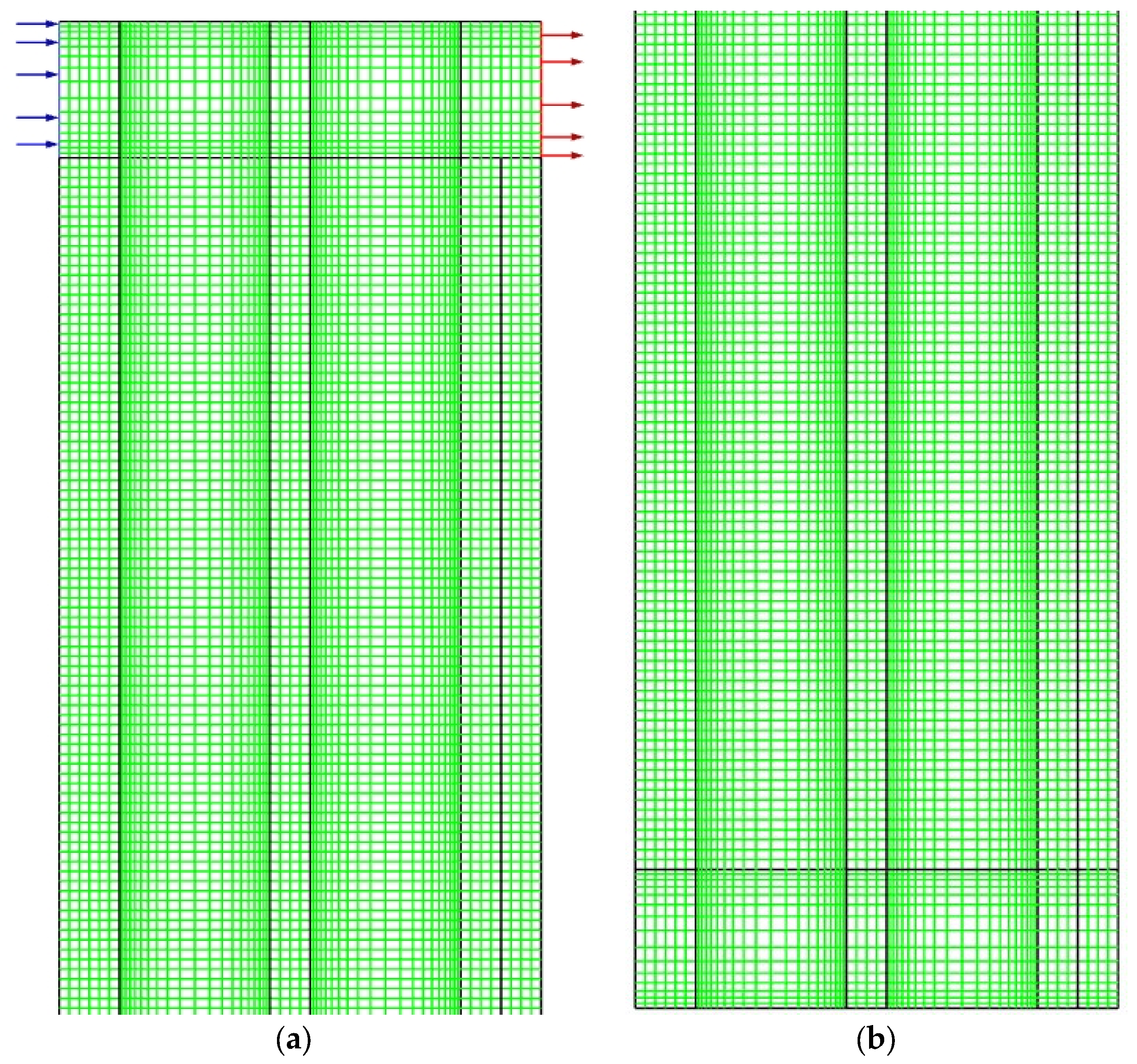
The resolution of the equations governing momentum and energy conservation in the window and the generation of a stable numerical solution require the construction of a grid containing a sufficient number of meshes, since the numerical result obtained must be independent of the mesh. However, hardware constraints such as calculation resources have led us to optimize mesh density and architecture. It is essential for the mesh to be tightened in all zones where the variables have high gradients, in particular in the vicinity of walls and in those zones where the fluid flow direction changes (recirculation zones). For this purpose, the supply air window was divided into six zones: the window entrance and exit, two at the window bottom with the passage of air from one air gap to the next, and the vertical zones between the three glazings. This cutting was developed with the Ansys-Workbench tool. The window configuration was generated by means of the DesignModler component; this module offers several possibilities with respect to not only the creation of the geometry and the prior definition of model boundary conditions but also mesh generation and parameterization. In order to verify the independence of the numerical results, six grid variants with different densities were produced. The mesh density was varied from 46,000 to 338,100 cells, which served to ensure the stability of the digital solution obtained. Generally speaking, the mesh specification depends on the complexity of the model geometry. Figure 5a,b present the architecture of the mesh generated in the supply air window, as observed by the elongation ratio of the component: a height-to-thickness ratio on the order of 25. An initial close-up is shown on the top of the window and a second at the window bottom. In the six grid variants studied, a structured quadratic grid was considered, i.e., in the window’s two air gaps, the grid dimensions are uniform in the flow direction. For the solid zones of the three panes, the mesh size remains uniform and homogeneous in both directions. Special attention has been paid to the zones of boundary layers close to the walls. A boundary layer mesh corresponding to y+ ≈ 1 (Equations (9) and (10)) and comprising at least 10 cells in the region close to the wall affected by the viscosity was configured. The boundary layer thickness was subdivided into several thin cells, given that temperature variation through the thickness of the layer is small and conductivity is high. This thickness was determined according to the conditions described in the Ansys-Fluent guide [38] for turbulent flows and in pipes undergoing a directional change:
y + = ρ . U τ . y μ
U τ = τ w ρ
This determination then made it possible to derive the size of the initial mesh of the viscous underlayer to be on the order of 0.5 mm; for the other zones, an expansion rate of 1.05 was applied to all other zones outside the boundary layers. The following figure (Figure 6b) indicates that for the dimensionless value of y+ with respect to surface 5 (the same applies for faces 2, 3 and 4), the values obtained are all less than unity, which means that the mesh is sufficiently refined near the walls and, moreover, that the first node is located in the viscous boundary sublayer. Let us recall that this method was used for an “enhanced wall treatment”, with a value of y+ ≈ 0.4.
As regards mesh independence, Figure 6a shows the comparison between the heat flux results obtained on face 4 (continuous line) and face 5 (dashed line) for the various grids. It can be noticed that for a mesh density of 46,550 (cells), the evolution of the heat flux curve with respect to face 5 reveals a disturbance in the bottom part of the window. This finding is undoubtedly related to the insufficient meshing over this zone. Beyond this lower zone of the window, all heat flux curves converge towards the same evolution. From a mesh density of 71,050, all curves obtained with respect to faces 4 and 5 yield the same evolution. The relative error between these curves with respect to face 5 remains less than 1%; similarly, the various flux curves obtained with respect to face 4 display an error less than 2%. Based on this sensitivity analysis, we opted for a density of 71,050 cells during the remainder of the simulations.

3.2. Temperature Measurements and Heat Flux

Figure 7 and Figure 8 show the experimental temperature measurements obtained in the window when steady state has been reached with a volume flow rate of Q = 62 m3.h−1 and a power injected into the heating glazing of 475 W.m−2 over a 3 h period. The system initialization phase has been eliminated in order to simplify data analysis. From Figure 7, it can be observed that the air temperature obtained is clearly stable throughout the acquisition period, except for the thermocouples, which had been placed at the center of air gaps, i.e., at the heart of the flow in the window. The recorded signals display some very low-amplitude wave movements due to the temperature variation of the fluid as it passes through the window. It was found that the variation in temperature measurements remains small for the thermocouples, whether placed in the cold cell (Text) or the hot cell (Tin), even for those temperatures recorded in the air gaps. This stabilization of temperature measurements validates the effectiveness of the measuring device designed for the window. As regards the surface temperature measurements on the three panes, the temporal evolutions were recorded in Figure 8. These temperatures were measured by thermocouples integrated into the flux meters and also proved to be very stable.
Let us note here that the surface temperature values evolve gradually, increasing from face 1 to face 6 (T1, T2, T4, T5 and T6, respectively); similarly, for face 5 of the heating pane, a very distinct change is observed in the surface temperatures along the vertical (T7, T8, T9, T5, T10 and T11, respectively). These thermocouples output increasing values over the entire heated height, from the bottom (T7) of the window to its top (T11).

3.3. Turbulence Modeling

The following figures (9 through 14) present a sensitivity analysis based on the choice of turbulence models available in the Ansys-Fluent tool and their efficacy in describing the physical phenomena involved in the window. As described above, we opted for three families of turbulence models. In the first family, grouping k-ε models (STD, RNG, REA), a standard function was used for treating the physical phenomena at the wall. The second family is essentially identical to the first but includes a so-called enhanced wall treatment. Lastly, the third family groups the models k-w (STD, SST, GEKO).
Figure 9 shows the evolution in the experimental and numerical temperatures obtained along faces 1, 2, 4, 5 and 6 of the three panes (see Figure 3). When using k-ε models with a standard wall treatment, some highly significant quantitative differences appear, mainly in comparison to the heated glass (pane numbers 3, f5 and f6). This temperature difference between the experimental and numerical results starts at the bottom of the heated window and increases as it moves towards the window top. For face 6 (f6), in this case, a comparison is nearly impossible, with the temperature differential between the experimental and numerical results lying on the order of 6 °C. For panes 1 and 2 (f1, f2 and f4), the temperature differential, less than previously, is on the order of 2 °C max. For the heat flux results, comparisons of the three k-ε models with a standard wall law are shown in Figure 10; the same remark applies as above, as significant differences are visible on the curves between the experimental and numerical results with respect to the heating pane (f5). On the other hand, at the level of face 6 (f6), the numerical and experimental results are nearly identical, as is the case for faces f1 and f2. Similarly, Figure 10 shows that whichever k-ε model is used with a standard wall treatment, the evolutions in the numerical curves obtained with the three k-ε models are virtually identical, and this applies to the five faces f1, f2, f4, and f5.
In the second family of tests on the sensitivity of turbulence models, k-ε models were used with an enhanced wall treatment. The comparison results between the numerical and experimental curves are reported in Figure 11 and Figure 12.
Figure 11 reveals that the comparison between numerically and experimentally obtained temperature curves is much better than the previous comparison (Figure 9) for faces f1, f2 and f4. For face 5 (f5), the temperature change is divided into two parts: (1) the temperatures obtained experimentally and numerically in the upper half of the height of pane 3 (f5) are perfectly merged, while (2) in the lower half of pane 3 (f5), the differences are visible on the curves, most likely due to recirculation phenomena as the fluid changes direction in the U-channel of the window. On face 6 (f6), the temperature difference between the numerical and experimental curves is very large, i.e., on the order of 4 °C. As regards the comparison of heat flux results (Figure 12), a very good agreement was obtained between the experimental and numerical curves, with a very small deviation for the first test family (Figure 10). For faces f1, f2, f4 and f6, the comparison provides a deviation of less than 1%. For face 5 (f5), the relative difference between numerical and experimental results equals around 3%.
Figure 13 and Figure 14 present the last family of tests using k-w models. Overall, in terms of comparison, a very good agreement exists between the results of the numerical simulations and those obtained experimentally. In Figure 13, it can be observed that the evolutions in the temperature profiles recorded experimentally are correctly reproduced by the numerical simulations based on the k-w models, and this applies to the five faces of the three glazings (f1, f2, f4, f5 and f6, respectively). For faces 1 and 2 (f1, f2, f4), all experimental and numerical results have been merged, except for face 4. The curve obtained by the k-w SST model reveals a difference in the upper area at the window exit. For faces 5 and 6 (f5, f6), the three turbulence models (STD, SST and GEKO) yield the same evolutions as for the experimental curves, with quantitative differences visible on certain curves. The smallest relative difference between the experimental and numerical results is obtained via the GEKO model and lies on the order of 3%. In the first conclusion on this sensitivity analysis, it can be stated that the results of comparisons of its turbulence models with the experiment indicate a very good agreement with the k-w models; this finding applies to all measurements (temperatures and heat fluxes) conducted in the window. The smallest relative deviation is obtained with the GEKO model; in contrast, the k-ε turbulence models with a standard wall law reveal a considerable flaw in the estimation of temperatures and heat fluxes in the window. For the remainder of the present simulations, the GEKO model has been used.

3.4. Analysis of Heat Flux and Temperature Results in the Heating Window

Simulations (Figure 15 and Figure 16) were carried out in order to confirm the reproducibility of the phenomena observed in the window. These simulations correspond to stabilized thermal and aeraulic conditions and are obtained on the basis of average values calculated during 3 h of data acquisition with a time interval of 30 s, which corresponds to means over 360 points.
At first glance, these results are consistent, and the phenomena identified by the numerical simulations are confirmed by the experimental tests:
The air recovers little heat in the first cavity. The evolution of air temperature is characterized by an increase at the top of the window and a decrease over the lower part. This phenomenon is becoming less and less noticeable as the air flow increases.
The preheating of the air takes place mainly on the second air plate.
The difference in wall temperatures in the first air gap is small, while that in the second air gap is greater.
For the heating window, disturbances are noted on both the temperature and heat flux curves at the bottom of the window. This phenomenon is most likely correlated with the formation of recirculation zones at the level of the passage from air gap 1 to air gap 2.
The following Figure 17, Figure 18, Figure 19 and Figure 20 show the comparison between numerical and experimental results in both temperature and flux for two heating powers different from the one previously imposed. For Figure 15 and Figure 16, the injected power is on the order of 190 W.m−2, whereas for Figure 17 and Figure 18, it lies on the order of 320 W.m−2. As seen in these figures, in the majority of test cases under turbulent conditions, the CFD simulations reproduce very well the trends obtained experimentally, regardless of the injected heating power. As also observed from these figures, in the majority of the cases tested in the turbulent regime, the CFD simulations reproduce very well the trends obtained experimentally, at whatever heating power is injected. For the temperature curves, in both cases (i.e., Figure 17 and Figure 19), similar profiles can be observed. The comparison between temperatures on face 5 is markedly better in the second case (P = 320 W.m−2). The temperature difference between experimental and numerical values is near zero over the upper half of the window height, i.e., preheating of the air in this upper zone is practically complete, and the temperature curve yields a rather flat profile. In contrast, in the lower half of the window (face 5), temperature differences are highly visible on the curves for both cases tested. This finding can be explained in several ways:
(1)
The change in fluid direction in the U-shaped duct. It is known that the two gaps are two rectangular cavities separated by a central window, with the connection between the two air gaps being “abrupt” without any zone of curvature to reduce the pressure drops.
(2)
The window at the bottom is equipped with wedges that support the central glazing at its extremities. This configuration may give rise to turbulence when air passes underneath this window. Such a division of the flow field in the U-shaped duct occurs just before the preheating of the air, which generates a very significant modification in the flow structure and dynamics.
(3)
The mode of operation of the heating window within this low zone remains too complex to identify. In fact, it would be worthwhile to explore this zone finely by means of measuring the velocity and temperature fields in order to understand the thermal and dynamic behavior in this zone and determine whether optimized exchanges are feasible.
(4)
Experimentally speaking, 3D effects are probably also correlated with the presence of the wooden frame. This is the case even when the measurements and simulation results relate to the mean behavior of the central zone window in two dimensions. However, for the first and second glazings, the comparisons of experimental and numerical temperature profiles show very good agreement in all three cases studied (P = 190 W.m−2, 320 W.m−2 and 475 W.m−2).
Figure 16 and Figure 18 present the comparison between the heat flux profiles obtained experimentally and numerically in the two injected power cases (P = 190 W.m−2 and 320 W.m−2). These profiles are determined based on the three windows, as mentioned in the caption of each figure. At first glance, in both figures, a very good agreement is found between the experimental and numerical results. On the heat flux curves, the profiles measured experimentally and numerically at the bottom of the window reveal a disturbance that spreads over the first few tens of centimeters of height. This sensitivity is undoubtedly related to the fluid recirculation zones within this zone, which induce a local decrease in temperature. The relative difference in flux values is estimated at less than 3%, which is a very satisfactory result.

3.5. Evaluation of the Heat Transfer Coefficient in the Heating Window

Figure 21 and Figure 22 present the evolution of the convective heat transfer coefficient in the second air gap. In Figure 21, the calculation of the exchange coefficient is based on the experimental method using Equations (11) and (12). This determination of the exchange coefficient was performed in relation to face 5 for an injected heating power in the glass of 475 W.m−2 and a flow rate of 62 m3.h−1. In Figure 22, the calculation of the exchange coefficient is based on the correlation of Shah and London [39] (Equation (13)), with respect to faces 4 and 5 (f4; f5) for three values of injected power (190, 320 and 475 W.m−2), respectively, (Figure 22a–c) and a flow rate of 62 m3.h−1. For the first method using Equations (11) and (12), it is important to remember that the classical formulation of the exchange coefficient, called “Newton’s linear formulation”, is always somewhat delicate in its application. Indeed, the main difficulty stems from the local estimation of the reference fluid temperature for a zone of finite dimensions (Equation (12)) at a given level in the air gaps. This value is the average temperature over the section of cavity surface S, with each temperature being weighted by the local velocity u(y). This is the temperature used to evaluate the enthalpy of the fluid at the axial position. From a numerical standpoint, the calculation of mixing temperature tends to be simplified. The temperature distribution and vertical velocity components in the mixing section are obtained directly via the temperature and velocity fields, which will serve to directly access the hc coefficient. From an experimental standpoint, the determination of mixing temperature remains very complex, if not altogether impossible (Equation (12)).
The calculation of these reference temperatures for the fluid requires defining a mixing zone; however, the choice of dimensions of these zones remains arbitrary, and the measurement tends to remain local. On the other hand, the measurement of surface temperatures is simpler, with very thin thermocouples being placed directly on the glass. Note: The situation would be more complex in the case of an incident solar flux of SW (shortwave) radiation, which would be absorbed by the measurement probe. This complexity of calculating the convective heat transfer coefficient using this method reveals a very large discrepancy between the experimental and numerical results of the exchange coefficient (Figure 21), which in turn explains the errors committed in estimating the mixing temperature within the measurement area.
h c = φ c o n v e c t i f T s u r f a c e T f l u i d e r e f
T f l u i d e r e f = 1 U . S s u r f a c e u ( y ) . T ( x , y ) d x d y
To overcome these difficulties during the measurement of fluid temperature, we have opted for the latter method, based on a direct use of the surface heat flux values obtained by the fluxmeter sensors placed on the surface of the glazing. Based on the approach developed by Shah and London [39] for forced convection flows, we can derive the local Nusselt number, which yields the convection coefficient. Figure 22 shows the comparison between the numerical and experimental results of the convective heat transfer coefficients determined on face 4 of pane 2 and on face 5 of pane 3. Let us note that the evolution of convective heat transfer coefficients obtained experimentally is correctly reproduced numerically for the three tests carried out with different injected thermal powers. These results are very valuable not only numerically but experimentally since they demonstrate the possibility of determining the quantities of energy exchanged by virtue of overcoming the reference fluid temperature measurement problem (here mixing temperature), which a priori is essential to determining the value of a convective heat transfer coefficient.
N u 1 ¯ = 140 26 9 φ P 2 φ P 1 ;                     N u 2 ¯ = 140 26 9 φ P 1 φ P 2

4. Conclusions

This paper has presented a numerical study to model the thermal behavior and heat exchange phenomena within a heated parietodynamic window with triple glazing and different modes of turbulence in the steady state. Installed between two air-conditioned cells and instrumented with fluxmeters and thermocouples, the prototype was subjected to various power injections, ranging from 190 to 475 W.m−2.
A comparison of the results provided by the experimental device with the CFD simulations demonstrated the relevance of numerical modeling and its main hypotheses, namely: the heated parietodynamic window with triple glazing can be modeled in its current state as a ventilated window when considering a two-dimensional geometry and a turbulent flow.
The tests on various turbulence models showed significant variations. It turns out that the “GEKO” model is the most suitable for numerically reproducing the specificities of flow in the heating parietodynamic window. Indeed, in this particular context, the numerical tool is very well suited to taking into account the phenomena occurring in the fluid boundary layer and defining the wall laws.
Use of this model has made it possible to recover, with very good precision, the experimental results obtained in climate cells within a controlled environment. The model thus developed is now capable of representing the behavior of the window under various temperature and flow scenarios; it will prove invaluable in defining useful correlations that can then feed into “simplified” analytical models. The component can thus be a useful element in the dynamic thermal simulation of buildings, which in turn will make it possible to simulate the performance of the window over longer periods (a full heating season). Moreover, such capability will be feasible with very reasonable calculation times.
This study has also confirmed the extreme importance of fluxmeter thermal measurements in determining convective heat transfer coefficients by removing the need to measure the fluid reference temperature. Here, the equation described by Shah and London was experimentally verified; this equation had been drawn up on the basis of an analytical study of forced flow in a channel that was differentially heated between two vertical plates.

Author Contributions

Conceptualization, Y.C.; Methodology, S.Z., Y.C. and S.L.; Software, S.Z. and Y.C.; Validation, S.Z. and S.L.; Formal analysis, Y.C.; Investigation, S.L.; Resources, S.L.; Writing—original draft, S.Z., Y.C. and S.L.; Writing—review & editing, Y.C. and S.L.; Visualization, Y.C.; Supervision, Y.C. and S.L.; Project administration, S.L.; Funding acquisition, S.L. All authors have read and agreed to the published version of the manuscript.

Funding

This research (Project “VARIETO”) was funded by the ADEME (French Agency for the Environment and Energy Management) in the “New Emerging Technologies” program. S. Zeiny’s thesis was funded by the social landlord “Pas de Calais habitat”.

Acknowledgments

Thanks are expressed to both ADEME (French Agency for the Environment and Energy Management) and the social landlord “Pas de Calais Habitat” for their financial support for this research. Thanks to the company “Groupe Ridoret” for the realization of the prototypes.

Conflicts of Interest

The authors hereby declare that they have no known competing financial interests or personal relationships that could have appeared to influence the work reported in this paper.

Nomenclature

CFDComputational Fluid Dynamics
GekoGeneralized k-ω
ESP-rEnvironmental Systems Performance—Research
STCBScientific and Technical Center for Building
SSTShear-Stress Transport
RNGRenormalization Group
CMVControlled mechanical ventilation
R i Richardson number
R e Reynolds number
ρ Density, k g . m 3
g Gravitational constant, m . s 2
β Thermal expansion coefficient, K−1
T Temperature rise, K or °C
e Cavity thickness, m
l Length, m
μ Dynamic viscosity, k g . m 1 . s 1
V Velocity, m . s 1
Q v Heat absorbed or released at constant volume, J
U j Velocity in the x j coordinate directions, m . s 1
U i Velocity in the x i coordinate directions, m . s 1
U m Mean velocity vector, m . s 1 .
κturbulent kinetic energy
εdissipation
P Static pressure, Pa
S i j Viscous stress tensor
δ i j Kronecker delta
μtTurbulence viscosity, P a . s
C p Specific heat capacity, J . k g 1 . K 1
r Position vector
s Direction vector
s Scattering direction vector
s Path length
a Absorption coefficient, c m 1
n Refractive index
σ s Scattering coefficient, m−1
σ Stefan-Boltzmann constant, 5.67037442 × 10⁻⁸ kg s−3 K−4
I Radiation intensity, W . s r 1
T Local temperature, K or °C
ϕ Phase function
Solid angle, sr
y Absolute distance from the wall, m
U τ Friction velocity
τ w Wall shear stress, Pa
h c Convective heat transfer coefficient, W . m 2 . K 1
φ c o n v e c t i f Convective heat exchange rate, W
SSurface area, m 2
φ P 1 convective heat flux for first pane surface, W
φ P 2 convective heat flux for second pane surface, W
x, y, zCartesian coordinates, m
2DTwo dimensional
3DThree dimensional

References

  1. Powell, G.A. Automatic Ventilator Window. U.S. Patent 3,034,416, 15 May 1962. [Google Scholar]
  2. Boehm, R.F.; Brandle, K. Testing of air flow windows for evaluation and application. In Proceedings of the American Society of Mechanical Engineers (ASME) Solar Energy Division Conference, Reno, NV, USA, 27 April–1 May 1981; p. 12. [Google Scholar]
  3. Korkala, T.; Saarnio, P.; Siitonen, V. Air Intake Arrangements of the Supply Air Window from the View of Comfort and Ventilation Efficiency; Swedish Council for Building Research: Stockholm, Sweden, 1984; p. 7. [Google Scholar]
  4. Paziaud, J. Fenêtre à Isolation Dynamique par Circulation d’Air. FR Patent 8,205,279, 30 September 1983. [Google Scholar]
  5. Greffet, R. Etudes Expérimentale des Performances Énergétiques D’une Fenêtre Pariétodynamique. Ph.D. Thesis, Université de La Rochelle, La Rochelle, France, 2016. [Google Scholar]
  6. Gloriant, F.; Tittelein, P.; Joulin, A.; Lassue, S. Modeling a triple-glazed supply-air window. Build. Environ. 2015, 84, 1–9. [Google Scholar] [CrossRef]
  7. Andreeva, D.; Nemova, D.; Kotov, E. Multi-Skin Adaptive Ventilated Facade: A Review. Energies 2022, 15, 3447. [Google Scholar] [CrossRef]
  8. Zhang, T.; Zhao, Y.; Zhao, Y.; Wang, S.; Wang, J. A passive pivoted window for stabilizing the natural ventilation rate. Energy Build. 2022, 267, 112151. [Google Scholar] [CrossRef]
  9. Skaff, M.C.; Gosselin, L. Summer performance of ventilated windows with absorbing or smart glazings. Sol. Energy 2014, 105, 2–13. [Google Scholar] [CrossRef]
  10. An, Y.; Choi, H.; Kim, E.; Kim, T. Experimental analysis of seasonal temperature characteristics and cooling and heating energy consumption of a slim double-skin window. Energy Build. 2022, 256, 111681. [Google Scholar] [CrossRef]
  11. Praveen, R.P.; Keloth, V.; Abo-Khalil, A.G.; Alghamdi, A.S.; Eltamaly, A.M.; Tlili, I. An insight to the energy policy of GCC countries to meet renewable energy targets of 2030. Energy Policy 2020, 147, 111864. [Google Scholar] [CrossRef]
  12. de Llano-Paz, F.; Calvo-Silvosa, A.; Antelo, S.I.; Soares, I. The European low-carbon mix for 2030: The role of renewable energy sources in an environmentally and socially efficient approach. Renew. Sustain. Energy Rev. 2015, 48, 49–61. [Google Scholar] [CrossRef]
  13. Gloriant, F.; Joulin, A.; Tittelein, P.; Lassue, S. Using heat flux sensors for a contribution to experimental analysis of heat transfers on a triple-glazed supply-air window. Energy 2021, 215, 119154. [Google Scholar] [CrossRef]
  14. Michaux, G.; Greffet, R.; Salagnac, P.; Ridoret, J.-B. Modelling of an airflow window and numerical investigation of its thermal performances by comparison to conventional double and triple-glazed windows. Appl. Energy 2019, 242, 27–45. [Google Scholar] [CrossRef]
  15. Gloriant, F. Caractérisation et Modélisation d’une Fenêtre Pariétodynamique à Trois Vitrages. Ph.D. Thesis, Université d’Artois, Arras, France, 2014. [Google Scholar]
  16. Khalvati, F.; Omidvar, A. Summer study on thermal performance of an exhausting airflow window in evaporatively-cooled buildings. Appl. Therm. Eng. 2019, 153, 147–158. [Google Scholar] [CrossRef]
  17. Wei, J.; Zhao, J.; Chen, Q. Energy performance of a dual airflow window under different climates. Energy Build. 2010, 42, 111–122. [Google Scholar] [CrossRef] [Green Version]
  18. Wei, J.; Zhao, J.; Chen, Q. Optimal design for a dual-airflow window for different climate regions in China. Energy Build. 2010, 42, 2200–2205. [Google Scholar] [CrossRef]
  19. Barakat, S.A. Thermal performance of a supply-air window. In Proceedings of the 12th Annual Passive Solar Conference, Solar ‘87, Portland, OR, USA, 12–16 July 1987; Volume 12, p. 11. [Google Scholar]
  20. Raffnsøe, L.M. Thermal Performance of Air Flow Windows. Master’s Thesis, Technical University of Denmark, Kongens Lyngby, Denmark, 2007; p. 115. [Google Scholar]
  21. ISO-15099; Thermal Performance of Windows, Doors and Shading Devices—Detailed Calculations. International Organization for Standardization: Geneva, Switzerland, 2003.
  22. Southall, R.G.; McEvoy, M.E. Investigations into the functioning of a supply air window in relation to solar energy as determined by experiment and simulation. Sol. Energy 2006, 80, 512–523. [Google Scholar] [CrossRef]
  23. Bhamjee, M.; Nurick, A.; Madyira, D.M. An experimentally validated mathematical and CFD model of a supply air window: Forced and natural flow. Energy Build. 2013, 57, 289–301. [Google Scholar] [CrossRef]
  24. Khosravi, S.N.; Mahdavi, A. A CFD-Based Parametric Thermal Performance Analysis of Supply Air Ventilated Windows. Energies 2021, 14, 2420. [Google Scholar] [CrossRef]
  25. Cherif, Y.; Tittelein, P.; Lassue, S. Etude numérique des échanges convectifs au sein d’une fenêtre pariétodynamique de type Paziaud contenant un film chauffant. In Proceedings of the XIV ème Colloque International Franco-Québécois en Énergie, Baie St-Paul, QC, Canada, 16–20 June 2019. [Google Scholar]
  26. CSTB. Rapport d’Essais n°42913; Centre Scientifique et Technique du Bâtiment: Marne la Vallée, France, 1997. [Google Scholar]
  27. Flux Richardson Number—Glossary of Meteorology. Available online: https://glossary.ametsoc.org/wiki/Flux_richardson_number (accessed on 30 March 2023).
  28. Padet, J.; Cotta, R.M.; Chereches, N.-C.; El Wakil, N. Convection laminaire interne: Critères de sélection pour distinguer les régimes de convection naturelle, mixte ou force. In Proceedings of the Congrès de la SFT, Reims, France, 30 May–2 June 2005. [Google Scholar]
  29. CSTB. Rapport d’Essais n°35078; Centre Scientifique et Technique du Bâtiment: Marne la Vallée, France, 1995. [Google Scholar]
  30. Leclercq, D.; Thery, P. Apparatus for simultaneous temperature and heat-flow measurements under transient conditions. Rev. Sci. Instrum. 1983, 54, 374–380. [Google Scholar] [CrossRef]
  31. Cherif, Y.; Sassine, E.; Lassue, S.; Zalewski, L. Experimental and numerical natural convection in an asymmetrically heated double vertical façade. Int. J. Therm. Sci. 2020, 152, 106288. [Google Scholar] [CrossRef]
  32. Patankar, S.V.; Spalding, D.B. A Calculation Procedure for Heat Mass and Momentum Transfer in Three Dimensional Parabolic Flows. Int. J. Heat Mass Transfer. 1972, 15, 1787–1806. [Google Scholar] [CrossRef]
  33. Li, Z.; Liu, Y.; Zhou, W.; Wen, X.; Liu, Y. Thermal pollution level reduction by sweeping jet-based enhanced heat dissipation: A numerical study with calibrated Generalized k-ω (GEKO) model. Appl. Therm. Eng. 2022, 204, 117990. [Google Scholar] [CrossRef]
  34. Sharkey, P.S.; Menter, F.R. A numerical investigation of the turbulent flow around a scale model JBC hull using the Generalized k-omega (GEKO) turbulence model. In Proceedings of the 11th International Workshop on Ship and Marine Hydrodynamics (IWSH2019), Hamburg, Germany, 22–25 September 2019. [Google Scholar] [CrossRef]
  35. Patil, T.; Patil, V. Aerodynamic Performance Prediction of a Car Using GEKO Turbulence Model and Application of Gradient Based Optimisation for Improving Aerodynamic Drag; SAE Technical Paper 2021-26-0353; SAE International: Warrendale, PA, USA, 2021. [Google Scholar] [CrossRef]
  36. Menter, F.R. Two-equation eddy-viscosity turbulence models for engineering applications. AIAA J. 1994, 32, 1598–1605. [Google Scholar] [CrossRef] [Green Version]
  37. Launder, B.E.; Spalding, D.B. The Numerical Computation of Turbulent Flows. Rev. Comput. Methods Appl. Mech. Eng. 1974, 3, 269–289. [Google Scholar] [CrossRef]
  38. Ansys Fluent 19.0 User’s Guide; Ansys Fluent: Canonsburg, PA, USA, 2018.
  39. Shah, R.K.; London, A.L. Laminar Flow Forced Convection in Ducts: A Source Book for Compact Heat Exchanger Analytical Data; Academic Press: New York, NY, USA, 1978. [Google Scholar]
Figure 1. Schematic diagram of the various ventilated windows: (a) Paziaud window; (b) ventilated double-glazing window; (c) double-skin window; (d) double airflow window.
Energies 16 03243 g001
Figure 2. Instrumentation of the parietodynamic window: (a) Installation of heat flux and temperature sensors; (b) Heat flux sensors before painting.
Energies 16 03243 g002
Figure 3. The heating window: (a) experimental apparatus; (b) schematic diagram of measurements.
Energies 16 03243 g003
Figure 4. Physical model of the heating window.
Energies 16 03243 g004
Figure 5. Mesh architecture adopted in the heating window with inlet (blue arrows), outlet (red arrows): (a) upper zone; (b) lower zone.
Energies 16 03243 g005
Figure 6. Numerical test showing curves of: (a) mesh independence results; (b) y+ values for faces 4 and 5.
Energies 16 03243 g006
Figure 7. Variations in air temperature measurements during data acquisition.
Energies 16 03243 g007
Figure 8. Variations in surface temperature measurements during data acquisition.
Energies 16 03243 g008
Figure 9. Experimental and numerical temperatures for the three glazings, according to k-ε models with a standard wall function.
Energies 16 03243 g009
Figure 10. Experimental and numerical heat fluxes for the three glazings, according to k-ε models with a standard wall function.
Energies 16 03243 g010
Figure 11. Experimental and numerical temperatures for the three glazings, according to k-ε models with an enhanced wall treatment.
Energies 16 03243 g011
Figure 12. Experimental and numerical heat fluxes for the three glazings, according to k-ε models with an enhanced wall treatment.
Energies 16 03243 g012
Figure 13. Experimental and numerical temperatures for the three glazings, according to k-w models.
Energies 16 03243 g013
Figure 14. Experimental and numerical heat fluxes for the three glazings, according to k-w models.
Energies 16 03243 g014
Figure 15. Experimental and numerical temperature profiles for the three glazings, according to k-w models, P = 190 W . m 2 .
Energies 16 03243 g015
Figure 16. Experimental and numerical heat flux profiles for the three glazings, according to k-w models, P = 190 W . m 2 .
Energies 16 03243 g016
Figure 17. Experimental and numerical temperature profiles for the three glazings, according to k-w models, P = 320 W . m 2 .
Energies 16 03243 g017
Figure 18. Experimental and numerical heat flux profiles for the three glazings, according to k-w models, P = 320 W . m 2 .
Energies 16 03243 g018
Figure 19. Experimental and numerical temperature profiles for the three glazings, according to k-w models, P = 475 W . m 2 .
Energies 16 03243 g019
Figure 20. Experimental and numerical heat flux profiles for the three glazings, according to k-w models, P = 475 W . m 2 .
Energies 16 03243 g020
Figure 21. Convective heat transfer coefficient, using Equations (11) and (12).
Energies 16 03243 g021
Figure 22. Numerical and experimental convective heat transfer coefficient (as measured by thermal fluxes and using Shah and London’s correlations [39], for P values of: (a) 190 W.m−2, (b) 320 W.m−2, and (c) 475 W.m−2.
Energies 16 03243 g022
Disclaimer/Publisher’s Note: The statements, opinions and data contained in all publications are solely those of the individual author(s) and contributor(s) and not of MDPI and/or the editor(s). MDPI and/or the editor(s) disclaim responsibility for any injury to people or property resulting from any ideas, methods, instructions or products referred to in the content.

