Abstract
Positive displacement pumps produce pressure ripple that can be reduced with the attenuation of the generated flow ripple. This paper presents the application of a gas bladder hydraulic damper with the aim of reducing the oscillations of the delivery flow rate of positive displacement machines. This work is focused on the development of a 1D fluid dynamic model of the damper, which is based on the fundamental fluid motion equations applied for a mono-dimensional flow. In order to represent the fluid flow inside the damper, a particular evaluation of the sound speed has been implemented. Experimental tests have been performed involving an axial piston pump with the damper installed in the delivery pipe to validate the model; tests were carried out at different pump working conditions and with different gas precharge pressure of the damper. The test results confirmed the effectiveness of the device, and the comparison with numerical results demonstrated a good agreement. Simulations have been carried out to investigate the influence of various parameters on damper effectiveness.
1. Introduction
Positive displacement pumps generate a fluctuating flow rate that causes a pressure ripple; therefore, the reduction of the pressure oscillation can be obtained only with the attenuation of the flow ripple. Axial piston pumps, for example, generate flow ripple due to the pistons periodically discharging fluid from the suction to the delivery.
A wide amount of the literature presents solutions to reduce flow and pressure fluctuations caused by positive displacement pumps, a significant number of them involving geometric optimization of the machine itself. In the case of axial piston pumps, researchers have devoted attention to designing the port plate to facilitate a seamless transition of fluid pressure between the suction and delivery phases and vice versa [1,2,3]. For gear pumps, a very widespread type of pump, engineers have employed special grooves in the side bushings to enhance machine performance in this regard [4,5,6,7,8,9].
Another way of reducing pump flow and pressure pulsation is to employ external devices in addition to the pump and the hydraulic system. These solutions can be divided into two groups: active damping systems and passive damping systems, which this paper focuses on.
Active techniques entail employing controlled and externally powered mechanisms. A method presented in the works [10,11] involves high-frequency actuation of the oscillating plate angle in an axial piston pump through a switching valve to mitigate the flow. Various research endeavors explore the application of piezo-stack actuators to act pistons, thereby neutralizing the flow by engendering an out-of-phase flow signal [11,12,13].
Active techniques bear the advantage of delivering efficacious results irrespective of the pressure and frequency parameters of the working conditions, but they are generally complex and costly.
Passive techniques are simpler and cheaper because they demand no external control or power and do not need sensors for measurements. Frequently, passive methods damp the flow ripple by means of elastic components that interact with the flow. Nonetheless, such systems come with a drawback: they are often tailored to deliver peak performance within a specific range of working conditions, outside of which their effectiveness decreases.
Shang’s research [14] provides an illustration of this aspect where a spring accumulator is utilized to diminish the main harmonic of the flow ripple created by an axial piston pump. The mechanism further leverages the phase features of the suction and discharge flow ripple and pressure ripple to enhance performance. Alternatively, [13] proposed a distinct approach wherein the length and stiffness of elastic tubes are optimized within a hydraulic circuit to accomplish ripple reduction.
This paper explores the potential of gas-charged bladder hydraulic accumulators as a passive device for reducing flow and pressure ripple. The practice of implementing accumulators in hydraulic systems to mitigate fluid-borne noise and irregularities is widely established [15,16]. By acting as a low-pass filter in a fluid-filled line, an accumulator can compensate for peaks, both negative and positive, that may arise in the flow by storing or supplying the excess or deficiency of fluid, respectively.
More in detail, this paper focuses on a specific type of gas accumulator, the in-line bladder noise damper. Many studies have been conducted on this device, including modeling approaches to predict its bandwidth and acoustic attenuation performance. In previous works [17,18], different linear multimodal models have been proposed and validated through experimental procedures. Additionally, a method based on acoustic FEM and plane wave theory has been proposed in another study [19], and its results have been compared with experimental data.
The objective of this study is to create a 1D fluid dynamic model to examine the impact of the main features of an in-line bladder accumulator on its performance. Unlike models presented in the cited works, the model proposed in this paper can provide information about the flow evolution inside the damper and predict the effect that the device produces at its ends. The model incorporates the fundamental features of the hydraulic damper and is used to simulate the device’s behavior under various operating conditions. An experimental investigation is conducted to collect data with the double aim of checking the damper performance and validating the mathematical 1D fluid dynamic model.
2. Experimental Setup for Damper Testing
2.1. In-Line Bladder Damper Description
The damper presents features to reduce its size as much as possible while maximizing the pressure ripple reduction effect. A simplified scheme of the damper is shown in Figure 1. The gas (nitrogen) is circumferentially arranged, and it is separated from the liquid fluid by a rubber membrane. A perforated pipe acts as a support for the bladder when the gas precharge pressure is higher than liquid pressure, especially when the damper is not in use; the holes must be small enough to avoid bladder extrusion. This perforated sleeve affects the mass fluid exchange between the internal pipe and Chamber 1.
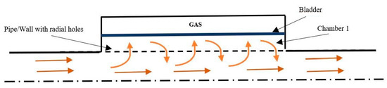
Figure 1.
Fluid flow inside the damper.
2.2. Experimental Activity
An experimental campaign has been carried out at the test bench of the University of Parma to investigate the damper performance. The damper installed is a model produced by Wilkes and McLean (5000 series). It was mounted on the delivery side of an axial piston pump (nine pistons) driven by a variable-speed electric motor, as shown in Figure 2. On the outlet side of the damper, a variable orifice was used to set the delivery pressure. Two high-frequency piezo-electric pressure transducers were installed upstream and downstream of the damper to measure the pressure ripple (Kistler 6005, 0–1000 bar, bandwidth 140 kHz). The damper was tested at different pump working conditions by varying the rotation speeds and delivery pressures, as shown in Table 1. Tests were performed at precharge pressure values of 150 bar and 100 bar to investigate the influence of gas precharge pressure on damper performance. The oil temperature during the tests was maintained at 50 °C. The damper’s gas temperature was not measured, but it was assumed to be equal to the oil’s temperature. High-frequency piezo-electric pressure transducers permit sampling at a rate of 20 kHz. Measurements were analyzed with FFT to identify the signal content in the frequency domain; the flat top window was applied to every record to reduce the leakage effect before performing the frequency analysis reported in Section 5.
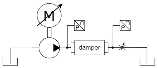
Figure 2.
Scheme of the circuit layout.

Table 1.
Pump working conditions.
3. Mathematical Model
3.1. One-Dimensional Fluid Dynamic Model
The mathematical model is based on a 1D approach that permits a detailed evaluation of the pressure evolution in time and space. The model implements the momentum equation and the mass conservation equation. The former for a horizontal pipe is the following:
While the latter is the following:
The general form of the continuity equation is valid for pipes with variable section area (A). In order to write the equation with the pressure variable in evidence (the state equation), the fluid must be introduced as the following:
The mass conservation equation becomes the following:
The second term could be written as the following:
Substitute the following:
This equation is often presented in a form where the speed of sound is used, as follows:
Therefore, the final form:
Exploit the total derivative:
The speed of sound has been computed considering the effective bulk modulus, and the pipe container elasticity effects can be computed by means of the following:
The pipe container is the bladder that separates the liquid from the gas; its effect depends on the gas pressure value. Assuming a polytropic transformation of the gas:
Differentiating Equation (13), the compressibility effects can be derived as follows:
and
With the gas transformations being very fast, they can be assumed adiabatic; therefore, the coefficient γ has been assumed equal to 1.4. The value of Kef is strongly affected by the term Kc.
The effective bulk modulus has been introduced in Equation (8):
The mathematical model with the elasticity of the pipe wall as a function of gas pressure can give relevant results in terms of pressure damping, but this model does not represent in sufficient detail the geometrical architecture of the damper and the fluid motion. Inside the damper, the liquid moves from the pipe to the bladder with a radial velocity component that could be represented only with a complex 2D model. The target of this research is to develop a model able to consider the geometrical features of the damper without a complex 2D CFD approach.
The fluid moving along the pipe (damper) presents a dominant axial component velocity. As previously described, the pipe presents a wall perforated with holes to connect the fluid inside the pipe to the bladder, Figure 2. When the instantaneous gas pressure is lower with respect to the instantaneous oil pressure, the oil moves through the holes acting on the bladder, the gas volume is reduced, and its pressure is increased. An opposite process occurs when the instantaneous liquid pressure is lower than the instantaneous gas pressure.
To model the damper functioning, the authors propose an original application of the fluid dynamic 1D model. The 1D modeling of the pipe permits one to evaluate the liquid pressure in time and space, while the gas pressure has been assumed as a function only of the time, then the gas pressure is assumed uniform inside the chamber and is only time-dependent. Following a liquid particle entering the damper with axial direction and assuming for the sake of clarity an instant when the liquid pressure is higher than the gas pressure, the oil also moves radially through the wall holes (Figure 1). This phenomenon could be modeled with a 1D approach assuming that the section available for the fluid is not constant but change over time. As a matter of fact, the sectional area made available by the wall holes acts as an increment of the cross-sectional area of the pipe, and vice versa when the gas pressure is higher than the oil pressure.
Therefore, in Equation (8), the term dA/dp is not null but could be positive or negative.
To implement this solution, the mathematical model computes the instantaneous flow rate through the wall holes, as a function of the wall holes’ size (making the model sensitive to this geometrical parameter) and as a function of the pressure difference between the instantaneous liquid pressure and the instantaneous gas pressure (making the model sensitive to the gas volume and the thermodynamic process adopted).
Then, the flow rate through the wall holes is managed to compute the term dA/dp in Equation (8). The instantaneous area variation has been calculated starting from the computed volumetric flow rate through the wall holes, and assuming that the fluid velocity is equal to the axial fluid velocity at the previous time step, an area could be determined. This area represents the variation of the cross-sectional area (A), so the term dA/dt is computed; this latter is associated with the instantaneous dp/dt, which permits the evaluation of the term dA/dp in Equation (8).
The liquid flow rate through the wall holes is calculated with the orifice equation for turbulent flow. The pressure difference through the pipe wall holes depends on the pressure of the liquid inside the pipe and the pressure of the liquid in the chamber between the perforated wall and the bladder (Chamber 1, Figure 1); in this chamber, the pressure could be assumed equal to the instantaneous pressure of the gas. The orifice equation is as follows:
The mass exchange through the wall holes is an unsteady-state process. Then, the liquid is subjected to inertial effects that could be computed with a correct evaluation of the instantaneous pressure difference applied to the transferred mass. These effects have been computed with an algebraic equation where the transferred mass, computed at each numerical time step, is subject to acceleration (Equation (18)), and the latter is computed on the basis of the instantaneous fluid velocity (Equation (19)):
where n is the instantaneous time step.
Then, the pressure difference between the liquid pressure and the gas pressure to compute the flow rate through the wall orifice is the following:
where and are the pressure values at steady-state conditions. is the inertial term:
The deformation of the bladder has not been considered because it is assumed that the bladder is not deformed during functioning but only moved.
The mass of the bladder could be computed by adding it to the mass of the transferred fluid, affecting the term . The mass of the bladder is assumed to be uniformly distributed through the pipe length. All these calculations are performed for each spatial discretization step.
The volumetric flow rate is exchanged between the pipe and Chamber 1 of Figure 1 through the wall holes and is also computed as a gas volume variation per unit time, being the volume of liquid equally transferred to the gas volume variation. The latter is used to compute the instantaneous gas pressure (making the model sensitive to the maximum gas volume (V0g), assuming an adiabatic thermodynamic gas transformation):
3.2. Unsteady Friction Losses
The momentum equation implements the friction losses that have been computed as frequency-dependent frictions [20,21] using Brunone’s model.
This model computes the unsteady terms on the basis of the instantaneous value of the velocity gradient (local inertia) ∂u/∂t and the convective term ∂u/∂x. The Brunone equation is the following:
where k (Brunone coefficient) could be defined by means of the Vardy coefficient (C*) as follows:
where for laminar flow, C* = 0.00476.
Whereas for turbulent flow:
3.3. Numerical Scheme
For the integration of the equations, an explicit first-order numerical scheme, called flux vector splitting [22], has been adopted. The explicit method involved is conditionally stable, so the Courant number has to be <=1, but values of the Courant number close to the unit by the solution become the most accurate.
The Courant number conditions are subjected to the variations in the speed of sound due to the variations of the term dA/dp, as reported in Equation (8). This aspect has been investigated to avoid a Courant number value over 1, which leads to instability problems. Because of the moderate speed of sound variations, it has been sufficient to set the Courant number at 0.95. Therefore, the values never exceed 1, and when it becomes slightly lower than 0.95, it could happen that the explicit method introduces a slight numerical diffusion that has been evaluated, not affecting the results.
A rigorous numerical solution should require a temporal and/or spatial grid that changes during simulation, but this complexity does not give any added advantage for this specific application.
Finally, the implemented numerical scheme is reported here:
The superscript n is referred to the temporal step, while the subscript i is referred to the spatial step.
4. Numerical and Experimental Results
In this section, the numerical results are reported and compared with experimental data obtained with the test apparatus described in sub-Section 2.2. All the data have been adimensionalized for confidentiality reasons.
The presented numerical results have been obtained by setting the boundary conditions at the inlet of the damper pipe in terms of the velocity profile. The velocity profiles have been calculated with an already-developed pump model that is not reported here because it is out of the scope of this paper [23]. The pump used during the test and for the simulations is an axial piston pump.
The first results presented concern the features of the adopted model. In Figure 3, the time history of the sound speed when the damper is not active (when the liquid pressure is lower than the gas precharge pressure) is reported. The little variations in sound speed are due to the effect of the instantaneous pressure value that affects the bulk modulus. In Figure 4, the sound speed is calculated with Equation (8) when the damper is active in two different cross-sectional areas, upstream and downstream, as reported. The average value is much lower with respect to Figure 3 because of the effect of the bladder that contains the fluid by means of the term Kc in Equation (8). Figure 3 shows a variation in the speed of sound that is due to the effects of the term dA/dp(t) in Equation (8). The instantaneous values of the sound speed affect the results in terms of pressure and fluid velocity, Equations (27) and (28).
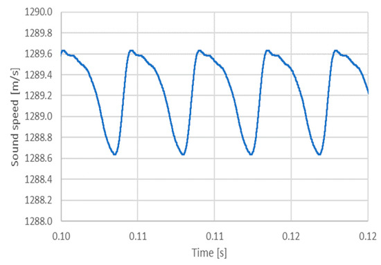
Figure 3.
Sound speed vs. time in a generic section of the pipe, damper inactive.
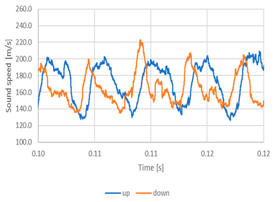
Figure 4.
Sound speed in upstream and downstream section, damper active.
In Figure 5, the pressure evolution in different cross sections of the damper when the damper is not active is reported. The damper is quite short, 0.1 m, and there are very few differences between upstream, downstream, and in the middle of the pipe damper (half). In Figure 6, the damper is active. The peak-to-peak values are reduced, and, thanks to the lower speed of sound, there are clearly visible differences between pressure oscillations at different sections of the damper: upstream, downstream, and in the middle of the pipe (half). The pressure evolution is also determined by the wave reflection effects. In this particular case, the peak-to-peak results are a little higher in the downstream section with respect to the upstream one.
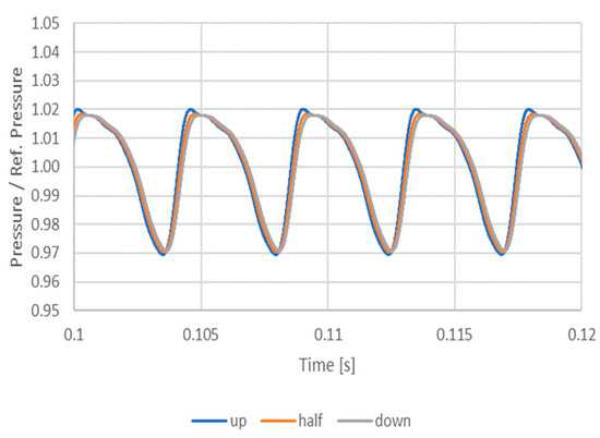
Figure 5.
Pressure evolution in different pipe sections with the damper inactive, pump speed = 1500 rpm.
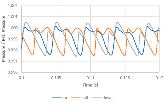
Figure 6.
Pressure evolution in different damper sections, pump speed = 1500 rpm.
In the following graphs, a comparison between numerical and experimental data is reported. The graphs report the FFT analysis of the pressure ripple, both numerical and experimental.
These graphs also report the case without a damper in order to present an easy evaluation of its performance. In Figure 7, Figure 8, Figure 9, Figure 10, Figure 11, Figure 12, Figure 13, Figure 14, Figure 15, Figure 16, Figure 17 and Figure 18, the legend “Exp. No sup.” represents the test carried out without the damper, while “Numerical No sup.” represents the numerical results with the damper inactivated.
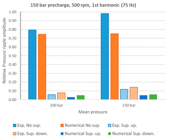
Figure 7.
FFT of the pressure ripple, 1st harmonic, pump speed = 500 rpm.
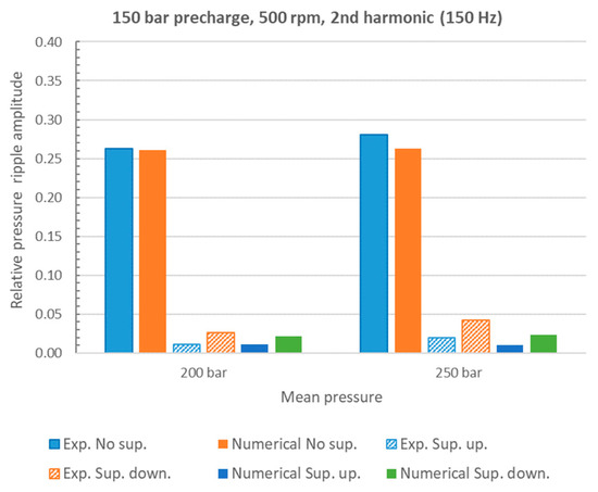
Figure 8.
FFT of the pressure ripple, 2nd harmonic, pump speed = 500 rpm.
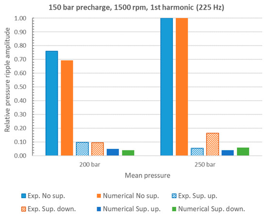
Figure 9.
FFT of the pressure ripple, 1st harmonic, pump speed = 1500 rpm.
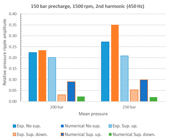
Figure 10.
FFT of the pressure ripple, 2nd harmonic, pump speed = 1500 rpm.
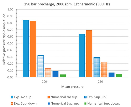
Figure 11.
FFT of the pressure ripple, 1st harmonic, pump speed = 2000 rpm.
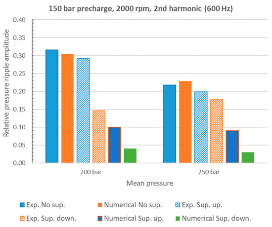
Figure 12.
FFT of the pressure ripple, 2nd harmonic, pump speed = 2000 rpm.
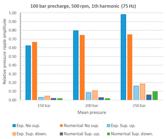
Figure 13.
FFT of the pressure ripple, 1st harmonic, pump speed = 500 rpm.
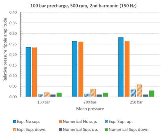
Figure 14.
FFT of the pressure ripple, 2nd harmonic, pump speed = 500 rpm.
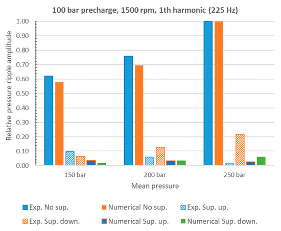
Figure 15.
FFT of the pressure ripple, 1st harmonic, pump speed = 1500 rpm.
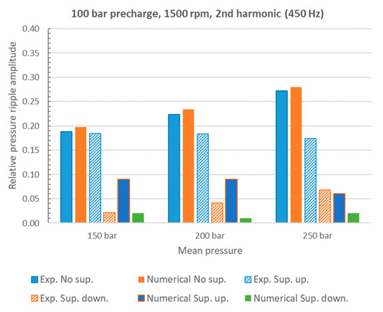
Figure 16.
FFT of the pressure ripple, 2nd harmonic, pump speed = 1500 rpm.
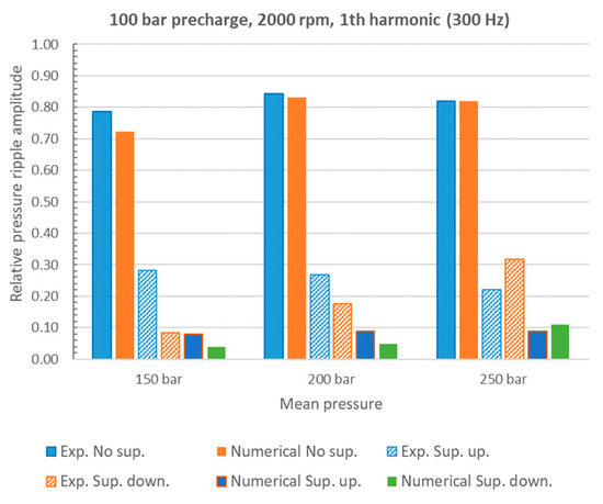
Figure 17.
FFT of the pressure ripple, 1st harmonic, pump speed = 2000 rpm.
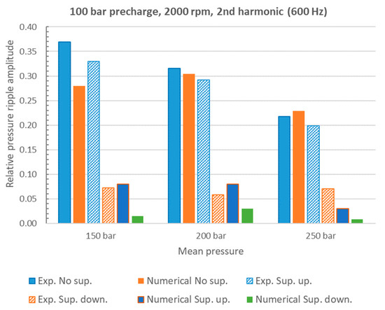
Figure 18.
FFT of the pressure ripple, 2nd harmonic, pump speed = 2000 rpm.
The experimental and numerical data without the damper is not significantly different between the upstream and downstream sections of the damper; therefore, there is only one value that is referred to the downstream section. When the damper is installed, the measured upstream and downstream pressure values are reported and simulated. The measurements of upstream and downstream pressures permit to have an exhaustive analysis of the damper performance.
The first case considered is with the precharged gas pressure set to 150 bar.
On the first harmonic at different pump speeds and delivery pressures in Figure 7, Figure 9 and Figure 11: the model well-reproduced the data without a damper. When the damper is installed, the experimental results present a strong reduction of the pressure amplitude, proving that the damper is able to reduce the pressure ripple, and also, the model reproduces a strong reduction of the pressure amplitude. Analyzing in more detail the results concerning the upstream and downstream sections of the active damper, it turns out that, on the one hand, the model slightly underestimates the experimental values. On the other hand, the model is able to reproduce the cases when the downstream pressure amplitude is higher with respect to the upstream pressure amplitude, Figure 7 and Figure 9.
By observing the results concerning the second harmonic, the model presents good results when the damper is not installed compared with the experimental results. When the damper is installed and active, similar considerations could be performed at a lower pump speed (500 rpm, Figure 8), where, again, the model reproduces a downstream pressure value a little higher than the upstream value. At higher pump speeds (1500 rpm and 2000 rpm, Figure 10 and Figure 12), the upstream sensor measures a higher-pressure value with respect to the downstream pressure. This particular situation can be reproduced by the model with a general underestimation of the pressure values. The second harmonic amplitude is always less than half of the first harmonic, and the downstream values are more important for the target of this solution.
Figure 13, Figure 14, Figure 15, Figure 16, Figure 17 and Figure 18 report the case where the damper precharge gas pressure was reduced to 100 bar. The results without damper are equal to the previous case, but they are reported in these graphs for easier comparison anyway. In this case, the damper starts to work at lower liquid pressure. Then, the results at a liquid pressure equal to 150 bar are now reported. When the damper works, similar considerations can be given for this case. The model reproduces the results in a satisfying manner, and also, in this case, the model presents a pressure amplitude reduction with a slight underestimation of the values.
The comparison between the performance of the damper at different gas precharge pressure values points out that the downstream pressures are always lower when the precharge gas pressure is higher (150 bar).
To further present the features of the developed model, a simulation assuming a damper with a double length, 20 cm, is presented in Figure 19. The time domain pressure in the downstream section presents lower peak-to-peak values in the case of 20 cm length with respect to the nominal case of 10 cm. It is also important to point out that the gas maximum volume is proportionally increased. This effect is stronger in Figure 20, where the length of the damper reaches 40 cm. The downstream pressure course presents a very low peak-to-peak amplitude. In Figure 21, the comparison is focused only on the downstream section for dampers of lengths equal to 10 cm and 40 cm, with the gas maximum volume changed in a proportional manner. Figure 21 also reports the curve identified as ‘10 cm V+’, which is referred to as a damper of length equal to 10 cm but with a maximum gas volume equal to the case of 40 cm. The best result is found with the case of a length of 40 cm and, as already reported, the maximum gas volume that is four times the case’s 10 cm length.
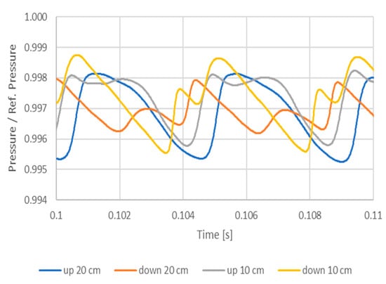
Figure 19.
Pressure evolution in the upstream and downstream sections with different damper lengths equal to 10 cm and 20 cm.
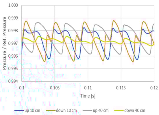
Figure 20.
Pressure evolution in the upstream and downstream sections with different damper lengths equal to 10 cm and 40 cm.
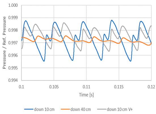
Figure 21.
Pressure evolution in the downstream section with different damper lengths and volume.
The FFT of the pressure ripple is reported in Figure 22, and the effects of the parameters length and gas volume are evident.
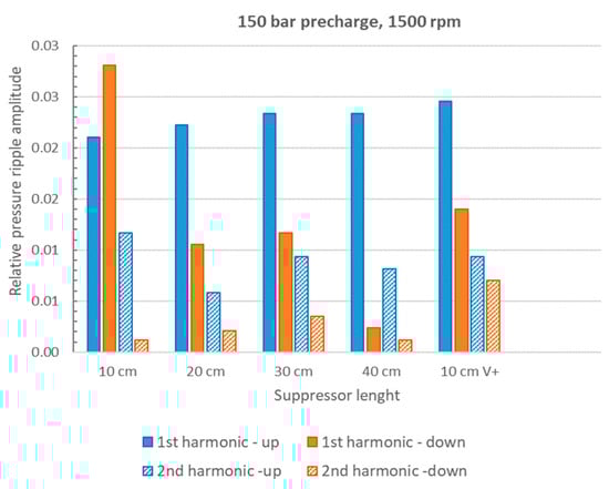
Figure 22.
FFT of the pressure ripple for different damper lengths and gas volumes.
5. Discussion
In this section, a detailed analysis of the results is presented.
With reference to the experimental and numerical results about the pressure at the upstream and downstream sections of the damper, they present a common trend increasing the pump speed in both cases at 150 bar and 100 bar gas precharge pressure. In particular, at low pump speeds, the upstream pressure is higher than the downstream pressure, and vice versa at higher speeds. A possible explanation can be found considering two physical aspects: wave reflection and pressure losses.
The pump is placed upstream of the damper and acts as a flow generator, and the restrictor is placed downstream of the damper and acts as a pressure generator. The restrictor, variable orifice, generates reflected waves that, in some cases, can produce higher pressure at the downstream section with respect to the upstream section of the damper.
The pressure loss effects are more relevant at higher pump speeds when the fluid speed is higher. As well known, in fact, friction losses increase with increasing fluid velocity. According to the results, this phenomenon is relevant at higher pump speeds.
The numerical model simulates the friction losses considering unsteady conditions (Equation (23)), while, on the wave reflection, the model needs the definition of boundary reflection conditions.
Further comments are needed to explain the performance of the damper at different gas precharge pressure values. Focusing on the downstream pressure ripple amplitude, it is always lower when the precharge gas pressure is higher (150 bar). These results are coherent with the thermodynamic process of the gas; when the precharge pressure is reduced at high liquid pressures, the gas works with a lower average volume. Equation (14), rewritten as Equation (29), shows that a lower value of the gas volume changes the compressibility of the gas and, as a consequence, its effects on the pressure ripple:
The drawback is that when the gas precharge pressure is higher, the damper working pressure range is obviously reduced.
6. Conclusions
In this paper, the performance of a hydraulic bladder damper has been investigated. An extensive experimental activity was carried out by insertion at the delivery pipe of an axial piston pump the damper. The damper presents a strong capability to decrease the flow ripple by reducing the harmonic content of the measured pressure ripple with a particular reduction of the first and second harmonic that represent the main signal content of the pressure ripple. A mathematical model has been developed to reproduce the behavior of the damper. The model is based on a 1D approach then the fluid motion equations are integrated into space and time, reproducing the instantaneous pressure and velocity of the flow in each spatial step inside the damper. The mathematical model has been implemented in a particular manner in order to reproduce the fluid flow inside the damper. The flow presents a radial component due to the interaction with the bladder. This behavior has been implemented assuming a variable section area available for the fluid flow, which affects the speed of sound and the pressure propagation inside the damper. The 1D model developed permits the simulation of the dampers’ behavior under different working conditions. Moreover, it considers the effects of many geometrical features such as the internal pipe diameter, pipe length, area of the wall holes, precharge gas pressure, the maximum volume of the gas, and mass of the bladder. The comparison between experimental and numerical results and simulations concerning the effects of some geometrical parameters shows the potential of the developed model.
The research is in progress with the aim of developing the modeling of connections between pump and damper and damper and variable orifice to better investigate the differences between the measured upstream and downstream pressures. This model will be used to investigate a reduction of the size of the damper and the possibility of developing new different architectures.
Author Contributions
Conceptualization, P.C. and M.R.; methodology, P.C. and C.M.V.; software, P.C.; validation, P.C.; writing—original draft preparation, P.C. and C.M.V.; writing—review and editing, P.C., C.M.V. and M.R.; supervision, P.C.; project administration, P.C. All authors have read and agreed to the published version of the manuscript.
Funding
This research received no external funding.
Data Availability Statement
Not applicable.
Acknowledgments
The authors would like to acknowledge the active support of this research by Casappa S.p.A., Parma, Italy.
Conflicts of Interest
The authors declare no conflict of interest.
Nomenclature
| A | Cross-sectional area |
| ρ | Density |
| u | Fluid velocity |
| a | Speed of sound |
| Cd | Discharge coefficient |
| p | Fluid pressure |
| m | Mass of the transferred elementary volume |
| K | Bulk modulus |
| Pipe wall holes area | |
| Acceleration of the transferred fluid mass | |
| C | Courant number |
| λ | Fluid friction losses |
| Re | Reynolds number |
| t | Time |
| V | Volume |
| γ | Polytropic coefficient |
| Subscript | |
| n | Temporal step |
| i | Spacial step |
| l | Liquid |
| g | Gas |
| 0 | Reference, initial condition |
| ef | Effective |
| c | Container |
References
- Harrison, A.M.; Edge, K. Reduction of axial piston pump pressure ripple. Proc. Inst. Mech. Eng. 2000, 214, 53–64. [Google Scholar] [CrossRef]
- Manring, N. The Discharge Flow Ripple of an Axial-Piston Swash-Plate Type Hydrostatic Pump. J. Dyn. Syst. Meas. Control 2000, 122, 263–268. [Google Scholar] [CrossRef]
- Johansson, A.; Olvander, J.; Palmberg, J.-O. Experimental verification of cross-angle for noise reduction in hydraulic piston pumps. Proc. Inst. Mech. Eng. Part I J. Syst. Control. Eng. 2007, 221, 321. [Google Scholar] [CrossRef]
- Borghi, M.; Zardin, B. Axial Balance of External Gear Pumps and Motors: Modelling and Discussing the Influence of Elastohydrodynamic Lubrication in the Axial Gap. In Proceedings of the ASME International Mechanical Engineering Congress and Exposition, Houston, TX, USA, 13–19 November 2015. [Google Scholar] [CrossRef]
- Zhao, X.; Vacca, A. Theoretical investigation into the ripple source of external gear pumps. Energies 2019, 12, 535. [Google Scholar] [CrossRef]
- Zhao, X.; Vacca, A. Numerical analysis of theoretical flow in external gear machines. Mech. Mach. Theory 2017, 108, 41–56. [Google Scholar] [CrossRef]
- Zhou, J.; Vacca, A.; Casoli, P. A Novel Approach for Predicting the Operation of External Gear Pumps Under Cavitating Conditions. In Simulation Modelling Practice and Theory; Elsevier: Amsterdam, The Netherlands, 2014; Volume 45, pp. 35–49. [Google Scholar] [CrossRef]
- Corvaglia, A.; Rundo, M.; Casoli, P.; Lettini, A. Evaluation of tooth space pressure and incomplete filling in external gear pumps by means of three-dimensional CFD simulations. Energies 2021, 14, 342. [Google Scholar] [CrossRef]
- Corvaglia, A.; Ferrari, A.; Rundo, M.; Vento, O. Three-dimensional model of an external gear pump with an experimental evaluation of the flow ripple. Proc. Inst. Mech. Eng. Part C J. Mech. Eng. Sci. 2021, 235, 1097–1105. [Google Scholar] [CrossRef]
- Casoli, P.; Pastori, M.; Scolari, F.; Rundo, M. Active pressure ripple control in axial piston pumps through high-frequency swash plate oscillations—A theoretical analysis. Energies 2019, 12, 1377. [Google Scholar] [CrossRef]
- Hagstrom, N.; Harens, M.; Chatterjee, A.; Creswick, M. Piezoelectric actuation to reduce pump flow ripple. In Proceedings of the ASME/BATH 2019 Symposium on Fluid Power and Motion Control 2019 FPMC, Sarasota, FL, USA, 7–9 October 2019. [Google Scholar]
- Casoli, P.; Vescovini, C.M.; Scolari, F.; Rundo, M. Theoretical Analysis of Active Flow Ripple Control in Positive Displacement Pumps. Energies 2022, 15, 4703. [Google Scholar] [CrossRef]
- Pan, M.; Ding, B.; Yuan, C.; Zou, J.; Yang, H. Novel Integrated Control of Fluid-Borne Noise in Hydraulic Systems. In Proceedings of the BATH/ASME 2018 Symposium on Fluid Power and Motion Control FPMC 2018, Bath, UK, 12–14 September 2018. [Google Scholar]
- Shang, Y.; Tang, H.; Sun, H.; Guan, C.; Wu, S.; Xu, Y.; Jiao, Z. A novel hydraulic pulsation reduction component based on discharge and suction self-oscillation: Principle, design and experiment. Proc. Inst. Mech. Eng. Part I J. Syst. Control Eng. 2020, 234, 433–445. [Google Scholar] [CrossRef]
- Rabie, M.G. On the application of oleopneumatic accumulators for the protection of hydraulic transmission lines against water hammer—A theoretical study. Int. J. Fluid Power 2007, 8, 39–49. [Google Scholar] [CrossRef]
- Yokota, S.; Somada, H.; Yamaguchi, H. Study on an active accumulator. JSME Int. J. 1996, 39, 119–124. [Google Scholar] [CrossRef]
- Marek, A.K.; Gruber, E.R.; Cunefare, K.A. Linear multimodal model for a pressurized gas bladder style hydraulic noise suppressor. Int. J. Fluid Power 2013, 14, 5–16. [Google Scholar] [CrossRef]
- Gruber, E.R.; Cunefare, K.A.; Danzl, P.W.; Marek, K.A.; Beyer, M.A. Optimization of Single and Dual Suppressors Under Varying Load and Pressure Conditions. Int. J. Fluid Power 2013, 14, 27–34. [Google Scholar] [CrossRef]
- Yi, X.; Bao-ren, L.; Long-long, G.; Teng-fei, T.; Hui-li, L. Acoustic attenuation performance prediction and analysis of bladder style hydraulic noise suppressors. Appl. Acoust. 2018, 134, 131–137. [Google Scholar]
- Zielke, W. Frequency-dependent friction in transient pipe flow. J. Basic Eng. 1968, 90, 109–115. [Google Scholar] [CrossRef]
- Benjamin, E.W.; Streeter, L. Fluid Transients in Systems; Prentice-Hall: Hoboken, NJ, USA, 1993. [Google Scholar]
- Hoffman, J.D. Numerical Methods for Engineers and Scientists; Mc Graw Hill: New York, NY, USA, 1992. [Google Scholar]
- Casoli, P.; Pastori, M.; Scolari, F. Swash plate design for pressure ripple reduction—A theoretical analysis. In AIP Conference Proceedings; AIP Publishing LLC: Melville, NY, USA, 2019. [Google Scholar] [CrossRef]


Disclaimer/Publisher’s Note: The statements, opinions and data contained in all publications are solely those of the individual author(s) and contributor(s) and not of MDPI and/or the editor(s). MDPI and/or the editor(s) disclaim responsibility for any injury to people or property resulting from any ideas, methods, instructions or products referred to in the content. |
© 2023 by the authors. Licensee MDPI, Basel, Switzerland. This article is an open access article distributed under the terms and conditions of the Creative Commons Attribution (CC BY) license (https://creativecommons.org/licenses/by/4.0/).