Mitigating Market Power and Promoting Competition in Electricity Markets through a Preventive Approach: The Role of Forward Contracts

Abstract

This paper proposes a novel approach to optimizing the structure of the electricity market by mitigating market power through the use of forward contracts. The IEEE 30 node test system is used as a case study for the paper, which employs nodal pricing and a Cournot model with recursive optimization. The findings show that forward contracts can reduce market power and lead to a more competitive market structure with fewer participants. The study emphasizes the importance of successor companies having a well-balanced mix of generation technology. Six players with a different generational mix are optimal in the constrained nodal pricing scenario, while five players with slightly different mixes are optimal in the Cournot case study. These findings have important implications for policymakers and industry stakeholders involved in the design and implementation of efficient electricity markets. Market power can be reduced by using forward contracts and establishing an appropriate number of market participants, resulting in more efficient and sustainable electricity markets. Overall, this study provides useful insights for improving electricity market structures and increasing competition in the electricity sector.

1. Introduction

In recent years, many countries have undergone electricity market restructuring in order to achieve competitive pricing and maximize welfare. Despite the significant resources invested in this process, market power has emerged as a significant issue, with the potential to keep electricity prices above competitive market levels. A crucial step in establishing a competitive electricity market is the division of the monopoly generation company (GenCo) into multiple competitive successor companies. As noted by [1], an adequate number of competing generators is crucial for mitigating market power and ensuring that wholesale markets are reasonably competitive. The regulatory reform and development of a competitive electricity market depend on creating an efficient number of competitors to mitigate market power and ensure that wholesale markets are reasonably competitive. In light of this, during the early stages of the restructuring phase, the state-owned GenCo should be restructured into several competitive successor enterprises that consist of multiple types of power plants. This split aims to create a competitive environment without the existence of dominant and pivotal players in the market that could exercise market power, and competition among generating companies will also ensure a sufficient mix of energy balance in the power system. As suggested by [1], it is advisable to address potential market power structurally before restructuring, in order to mitigate the potential adverse effects on prices and welfare.

Many countries have undergone electricity market restructuring with the goal of achieving competitive pricing and maximizing welfare. However, market power has emerged as a significant issue, resulting in market failure and preventing the attainment of maximum potential welfare gains. According to the authors of [2], market prices are often susceptible to unilateral market power, with pivotal successor companies exercising market power through strategic behaviors. To mitigate these effects, it is crucial for electricity regulators to design and implement a market structure that promotes competition and ensures efficient functioning of the market, while minimizing the influence of political considerations in decision-making processes. One crucial aspect of this is creating competitive successor companies in the wholesale electricity market through divestiture, as seen in the case of England and Wales [3]. However, it is important to note that simply divesting state-owned generation companies does not guarantee competitive behavior in the market, and efforts should also be made to design an optimal electricity market structure and generation technology mix to minimize market power through market power modeling.

Mitigating market power in the design of electricity markets is crucial for ensuring competitive pricing and maximizing welfare [2,4,5,6]. A crucial step in achieving this is the division of the monopoly GenCo into multiple competitive successor companies, as an adequate number of competing generators is essential for mitigating market power and ensuring that wholesale markets are reasonably competitive [1]. The configuration of players post-generation split should minimize market power, which can be achieved through ex-ante simulations prior to restructuring. Traditional measures of market power, such as the Herfindahl–Hirschman Index (HHI), may not accurately capture the dynamics of competition behavior in the wholesale electricity market due to factors such as inelastic demand, significant short-term capacity constraints, and high storage costs. Therefore, an alternative method, such as the Residual Supply Index (RSI), which was developed by the California Independent System Operator (CAISO), is considered more effective for market power mitigation in the electricity market [7,8,9]. The RSI is more effective because it considers the supply-side response to a market change, taking into account supplier behavior in relation to available capacity. Because it captures the incentives of suppliers to adjust their supply based on market conditions, this approach allows the RSI to provide a more realistic assessment of market power. As a result, in the design of electricity markets, the RSI is a better measure of market power and more effective in mitigating market power [10]. It is important for government and electricity authorities to take these considerations into account in determining the optimal configuration of the wholesale electricity market from a state-owned electricity company.

A review of the literature on market power mitigation reveals that most studies focus on corrective measures to address market power after it has already emerged, rather than preventive strategies to minimize its potential exercise. This is especially true for countries in the early stages of restructuring their electricity markets. A preventive approach to minimize market power is crucial for achieving maximum welfare for society and can serve as a more efficient approach towards establishing a competitive electricity market. The study by [11,12,13,14] presents a preventive approach to creating optimal successor companies prior to electricity market restructuring, but it does not incorporate the use of forward contracts as a tool to mitigate market power and optimize market structure. This present research aims to extend the work of [11,13,14] by incorporating the application of forward contracts in the proposed algorithm, which can potentially optimize the market structure with fewer market participants, thus reducing the exercise of market power. As such, this research makes a significant contribution to the literature by offering a novel and preventive approach to electricity market restructuring that accounts for the use of forward contracts as a tool to mitigate market power.

This research developed a bottom-up electricity market model that incorporates significant economic features and uses an ex-ante modeling approach to provide a realistic power system analysis. The model includes various market pricing structures such as locational marginal pricing and zonal pricing, taking into account the market boundaries and grid limitations of the specific power system. The computational simulation also includes strategic market behaviors, such as imperfect and perfect competition strategic interactions, and uses the Cournot model for ease of analysis. Incorporating the Residual Supply Index (RSI) and modeling the dynamics of the power system, where each node represents a load serving entity (LSE) and a supplier, present a novel approach to mitigating market power. This simplifies the calculations for load flow simulation. The model calculates load flow using a direct current approach and models marginal cost as a linear function based on heat rate curves, resulting in a more accurate calculation of generation costs. The model also employs a restricted-stylized approach for large-scale power system simulation, in which the transmission network model is based on the actual power system topology and one node represents a single high or extra high voltage power substation.

This research presents a novel algorithm for mitigating market power in electricity market restructuring by utilizing a balance of granular and easily accessible data. The algorithm, which can be implemented by any market designer in any state, utilizes publicly available datasets and takes into account the unique characteristics of the power network, grid code, and legal features. The economic modeling combines microeconomics, power engineering, law, policy, and mathematics, and incorporates forward contracts as a tool to reduce the number of market participants and create an optimal market structure in different competition scenarios. The algorithm can be applied in electricity markets that are still in a state of monopoly and considers the unique features of the power system topology. The ultimate goal of this research is to provide a practical solution for policymakers and market designers to mitigate market power and optimize market structure, building on previous research by [5,11,12,15].

The first chapter gives an overview of the research problem, objectives, and contribution. The literature review in Section 2 is thorough, covering relevant theories and models related to electricity market restructuring, market power, and forward contracts. The methodology section is detailed in Section 3, and it includes a bottom-up electricity market model that incorporates significant economic features and employs an ex-ante modeling approach for a realistic power system analysis. The section also discusses how forward contracts can be used to reduce market power and optimize market structure, as well as the Cournot model for strategic market behaviors. The study’s findings are presented in the results section in Section 4, including the optimal ownership structure and mix of successor companies, as well as the impact of forward contracts on mitigating market power. The results are analyzed in the discussion section of Section 5. Finally, the conclusions section in Section 6 summarizes the main findings, emphasizes the research contribution, and suggests future research directions.

2. Literature Review

2.1. Market Power and Preventive Antitrust Law

In his essay, the author of ref. [16] highlights the importance of economics in shaping antitrust policy, noting that economic theory plays a crucial role in shaping an economist’s perspectives on competition policy. He argues that antitrust laws are designed to promote competition among market players with the ultimate goal of reducing prices and increasing consumer welfare. Stigler also explains the distinction between preventive and corrective antitrust laws, noting that most US antitrust laws are corrective in nature and aimed at eliminating existing monopolies. However, he emphasizes the importance of antimerger statutes as a tool for preventing the formation of monopolies. This aligns with the argument in [17] that US antitrust policy is not designed to regulate or approve market structures and firm behavior across the economy; instead, the system relies on case law developed through enforcement actions which may have limitations in performing complex economic evaluations.

The European Commission’s approach to competition law, specifically with regard to merger policy, is focused on improving the structure of national markets through reactive measures. This means that the Commission only evaluates proposed mergers and assesses whether they will result in a better market structure than the current state. However, this approach has its limitations as the Commission cannot enforce a competitive market structure unless a merger proposal is brought forth. Additionally, the EU’s competition tools, such as directives, are flexible and rely on member states to take action and implement them. As a result, these tools may not be sufficient to create a truly competitive market, as argued by the authors of [18].

Effective antitrust provisions and institutions are crucial for maintaining a competitive market. Antitrust rules provide a legal framework for enforcing action and punishment for illegal activities, while antitrust agencies have the power to ensure compliance through enforcement actions. To achieve this, it is essential to have a solid economic foundation for antitrust laws and policies. An economics-based approach allows for the development of clear and understandable antitrust provisions and enables courts to evaluate and implement antitrust policy designs. This helps ensure that market players receive clear signals and guidelines regarding allowed and prohibited strategic actions.

Creating optimal antitrust laws, as outlined in [19], involves identifying and addressing anticompetitive behaviors in the market, while also considering the impact on market welfare. By assessing these behaviors and conducting law enforcement to intervene in harmful effects, the antitrust institution also creates a deterrent for misconduct behaviors. This approach not only addresses harmful market effects but also helps maintain a competitive market by preventing future misconduct.

Antitrust law is guided by two main theories of value: an efficiency-based theory, which prioritizes the maximization of welfare and efficient allocation of resources; and a standard for permissible strategic behavior, which aims to protect weaker economic entities and consumers from the market power of monopolies. Fines and sanctions play a crucial role in enforcing competition law prohibitions. According to the authors of [20], sanctions can prevent antitrust violations in three ways: by creating a deterrent effect, by having a moral effect, and by raising the cost of setting up and engaging in anticompetitive behavior. The threat of prosecution and fines can deter companies from violating antitrust laws, create a sense of moral commitment to compliance, and increase the cost of engaging in anticompetitive behavior, such as setting up and running cartels.

2.2. Forward Contract to Mitigate Market Power

The strategic interaction of market firms can be studied using game theory and industrial organization concepts. Firms’ strategic behavior is determined by their ability to predict the price and quantity decisions of other players. We chose the Cournot strategy for our study because of its simplicity and compatibility with power system characteristics such as generation and transmission constraints, voltage and stability conditions, generation ramp-up and ramp-down, contingency analysis, and commodity flow PTDF. The Cournot model involves quantity gaming, in which the strategic interaction is based on the supply provided by the company. This is in contrast to the Bertrand model, in which the quantity is the only decision variable, and each firm accepts the fixed price, resulting in no market power. While the Stackelberg model considers quantity gaming, it assumes a “leader” firm whose decisions correctly consider the reaction of “followers”, who are unaware of how their reactions affect the leader’s decision. This assumption may not hold true in practice, making the Cournot model a better fit for our research. Overall, by incorporating the effects of anticipation and strategic behavior among firms, the Cournot model with forward contracts can help to reduce market power in the electricity market and produce more realistic prices.

The matching of power supply with electricity demand is essential in the electricity market. To maintain this balance, power systems have objectives such as maintaining a stable frequency and voltage level. Power system dispatchers plan the export and import of electricity based on transmission characteristics and PTDF load flow. Additionally, the restructured electricity market is characterized by price volatility, particularly in the spot market. To mitigate this risk, forward contracts are important for retailers and suppliers [21].

In cases where market settings heavily rely on the spot market, as seen in the California crisis of 2000–2001, electricity market crises may occur. At the time, the system reserve margin was tight and there was a lack of forward contracts. The authors of ref. [22] suggest that implementing forward markets could have reduced or prevented the crisis. Forward contracts address three main issues in the wholesale market: investment, risk, and market power. In tight and scarce conditions, generator owners may accept profits below the true electricity price due to price cap regulations and adjustments from operators. Forward markets provide reliable payments and investment incentives for efficient entry, thus reducing this risk.

The use of forward contracts in the electricity market can help to reduce the market power of key players, as demonstrated by studies such as [23,24]. The Cournot model, which is widely used in the electricity market due to its simplicity and compatibility with power system characteristics such as generation and transmission constraints, voltage and stability conditions, and commodity flow PTDF, can be easily integrated with forward contracts. Additionally, the Cournot model is known to produce prices that are higher than would be expected with realistic demand elasticity, and forward contracts can help to make the model more realistic.

Forward contracts play a crucial role in reducing the ability of key market players to exercise market power, as demonstrated in [23] in their analysis of Cournot oligopoly behavior and in [24] in his study of the supply function equilibrium. In the electricity market, modelers often use the Cournot framework due to its simplicity and compatibility with power system characteristics, such as generation and transmission constraints, voltage and stability conditions, generation ramp-up and ramp-down, contingency analysis, and commodity flow PTDF. Incorporating forward contracts into large-scale Cournot power systems is also a convenient option. However, the Cournot equilibrium price is considered too high and output too low, when compared to realistic demand elasticity. Therefore, forward contracts can help make the model more realistic, as per [25].

In the long run, contracts can also increase new entry and competitive behavior, especially in the power plant investment sector, particularly in gas power plants. For example, in the first year after the establishment of the OFGEM (Office of Gas and Electricity Markets) in 1998, there was a significant investment of five GW gas power plants from IPPs and five GW from existing companies. This was due to the support provided by long-term forward contracts in the gas and electricity commodity market. However, as per the [24] model, contracts may also deter entry in cases where such deterrence is necessary for increasing efficiency.

3. Research Methodology

The optimized electricity market structure is based on the preventive approach developed by the authors of [11,12,13,14].

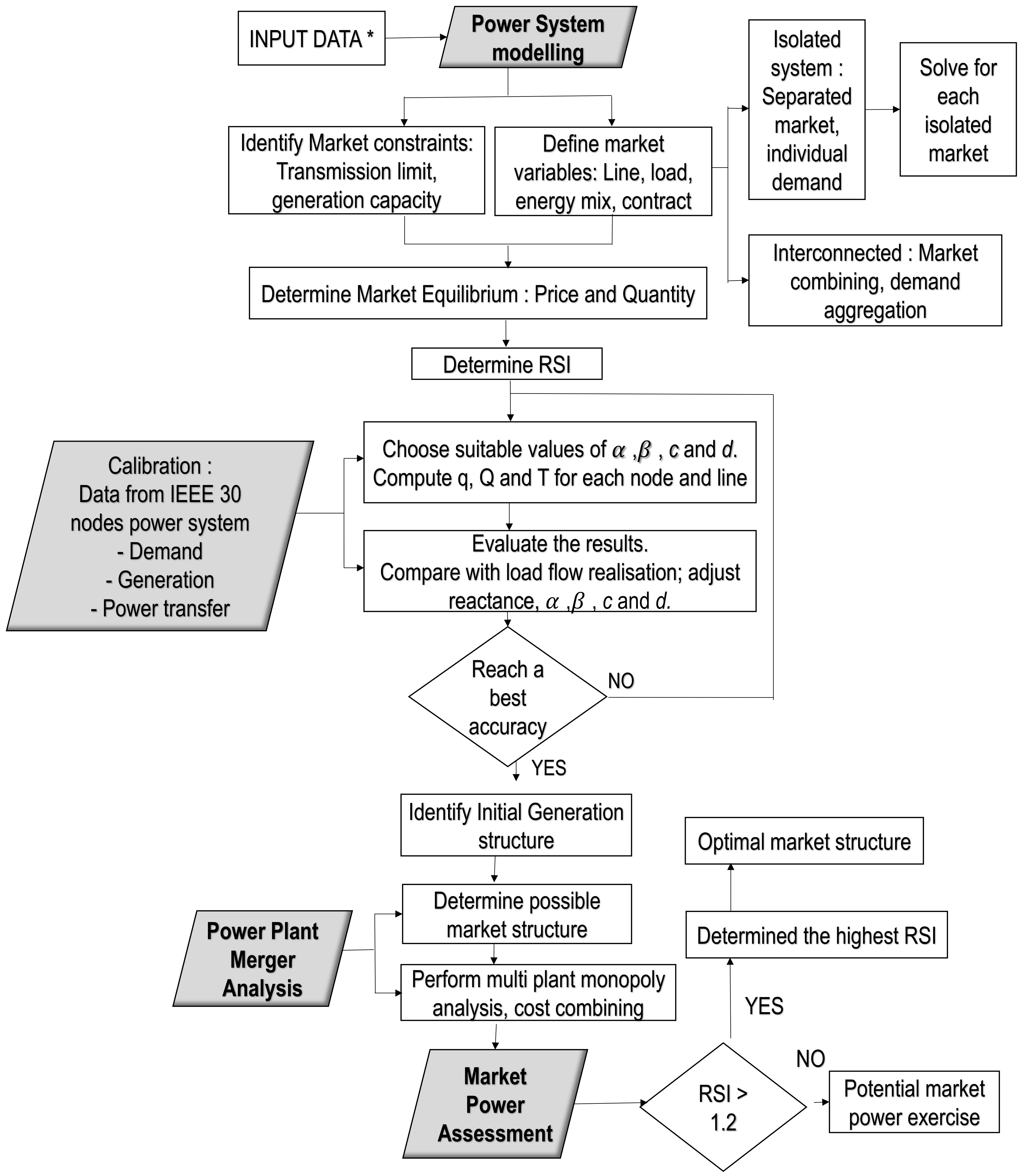
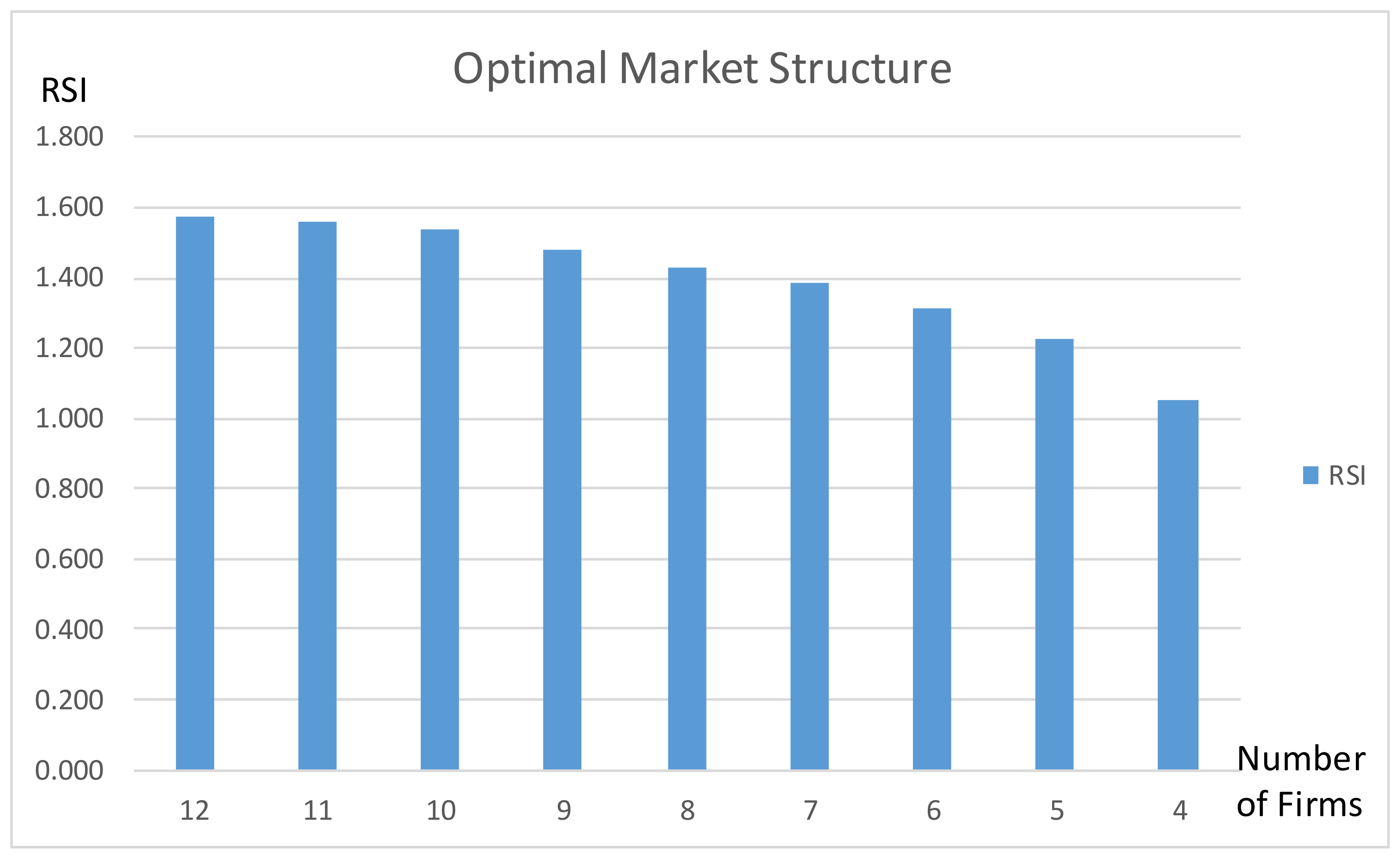
The conceptual algorithm outlines a four-step process for achieving the optimal market structure.

• The first step is to create a model of the nodal market using market characteristics and constraints. We developed perfect and imperfect (Cournot) competition models of the IEEE 30 nodes system by incorporating generation and transmission constraints. The perfect competition model is grounded in research conducted in [13,14,15,26,27,28,29,30]. The research on Cournot competition modeling served as the basis for our implementation of this approach in the study. Specifically, we relied on the work of [4,11,13,31,32]. The constraints related to generation include capacity, energy mix, and reserve margin, whereas transmission constraints encompass DC load flow, transmission limits, and line connections.
• The model is then calibrated to match the actual conditions of the power system in the second step. This includes examining market power behavior during peak loads. This step is critical for ensuring that the model accurately reflects the power system’s real-world conditions.
• The third step is to use a power plant merger analysis to examine potential market structure configurations. We assume that companies that own multiple power plants behave as multi-plant monopolists [33]. This step takes into account things such as the initial generation structure and the presence of independent power plants. The goal is to determine the best ownership structure and succession company mix.
• The final step is to assess market power using the Residual Supply Index (RSI) and consider any additional capacity investments that may be required. This step ensures that the market structure is competitive, and that welfare is maximized while addressing any issues with generation capacity and reserve margin. Based on the empirical study in [7,8,9], we used a screening process to determine the optimal market structure for each configuration. The screening process was based on an RSI threshold of 110%.

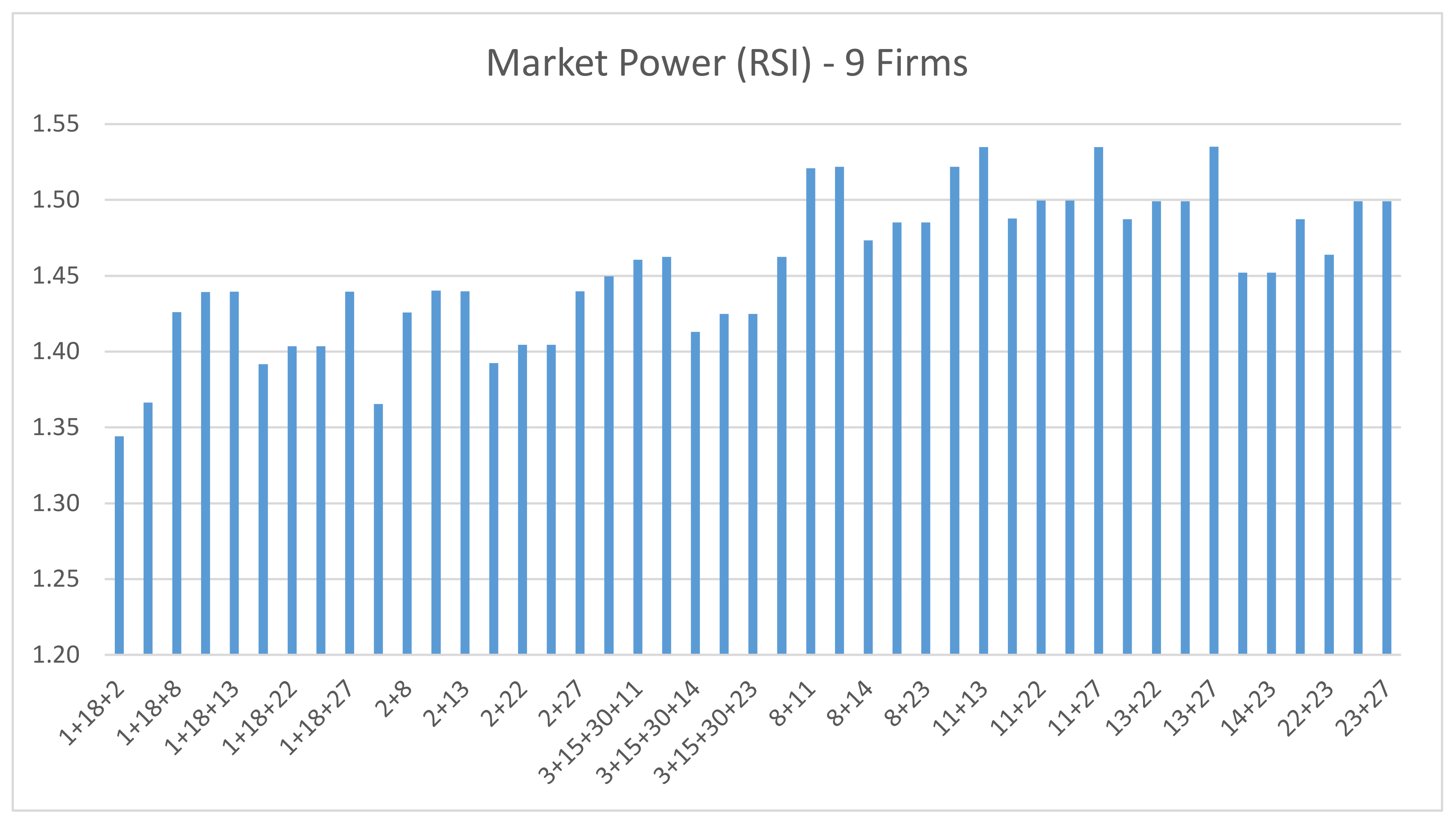
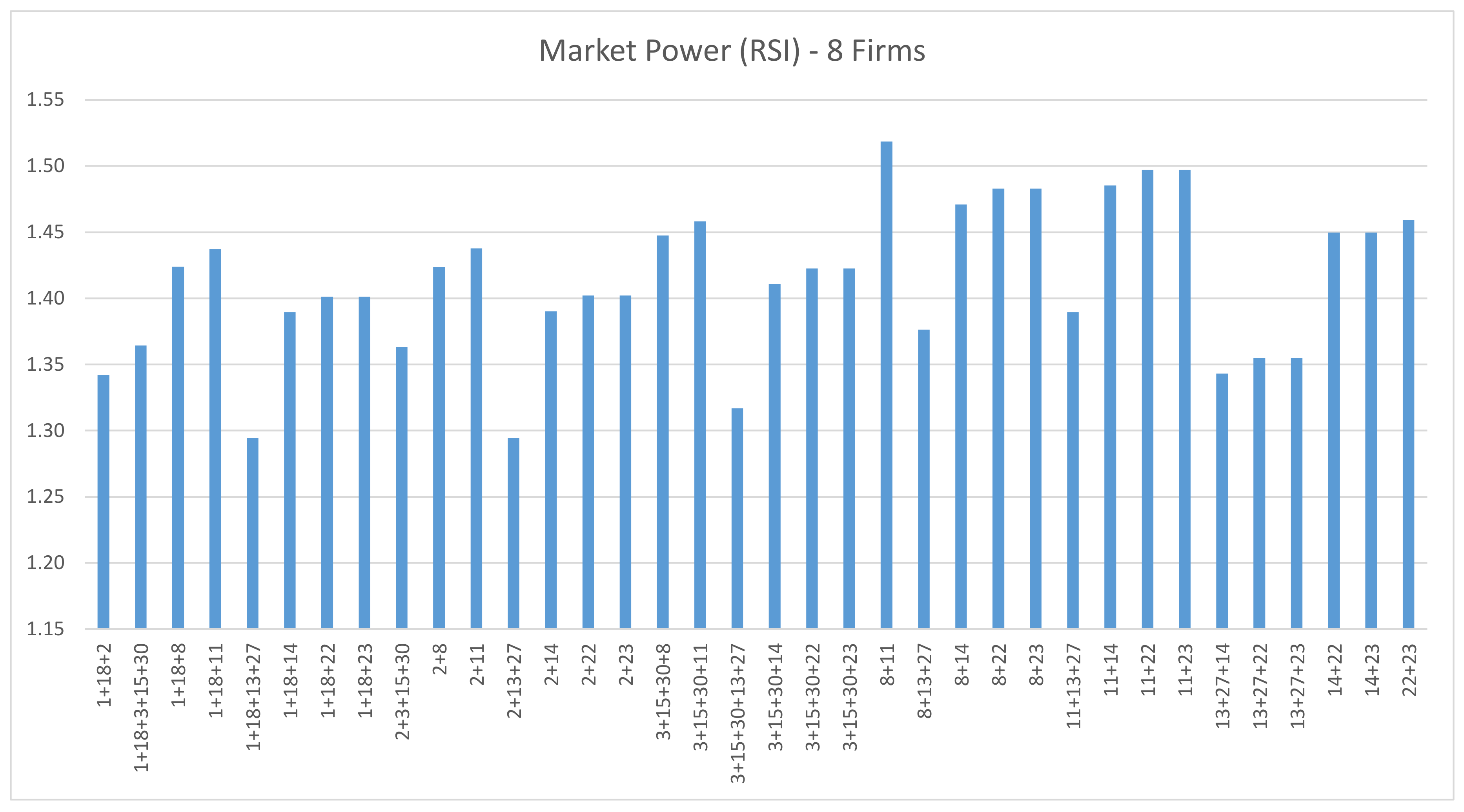
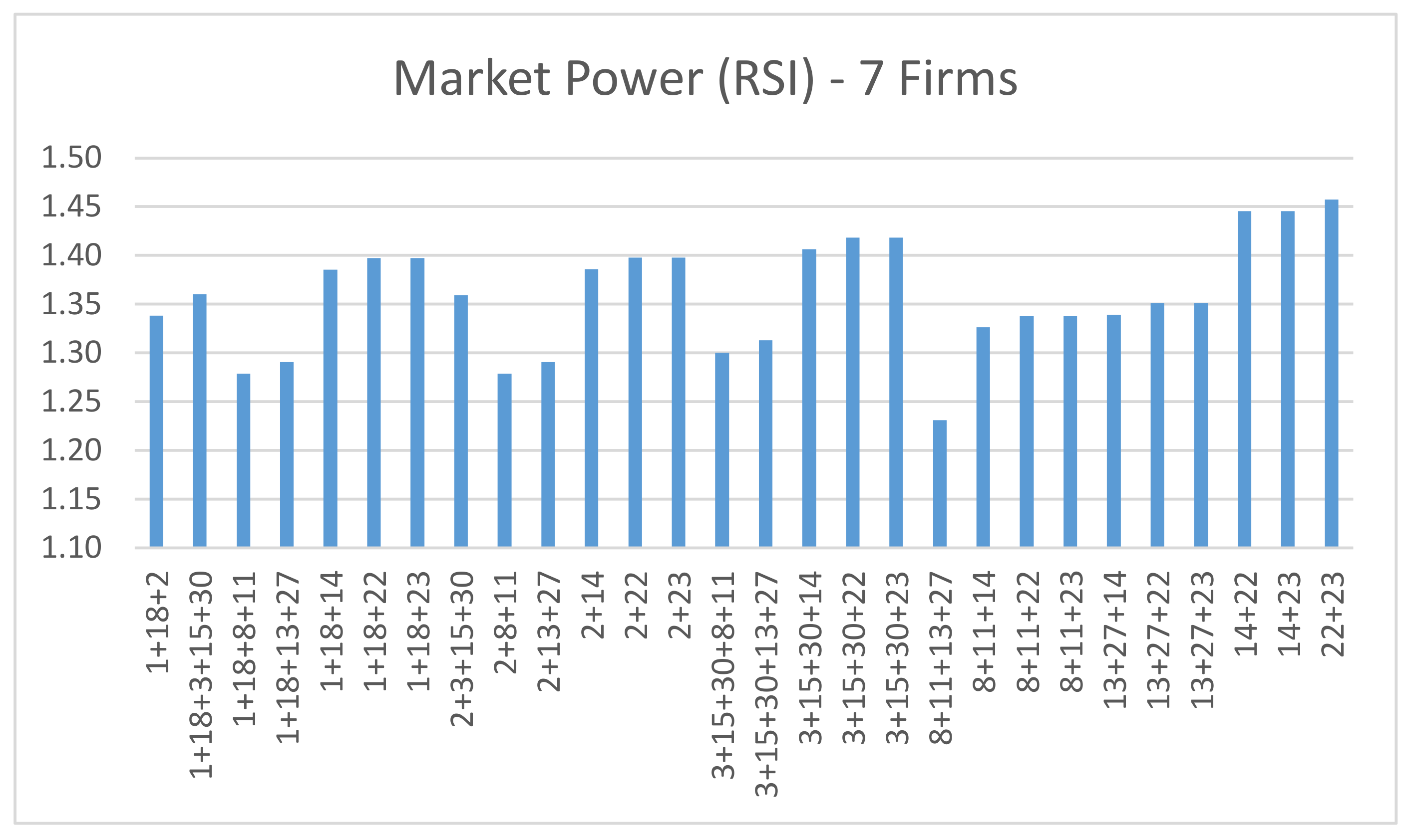
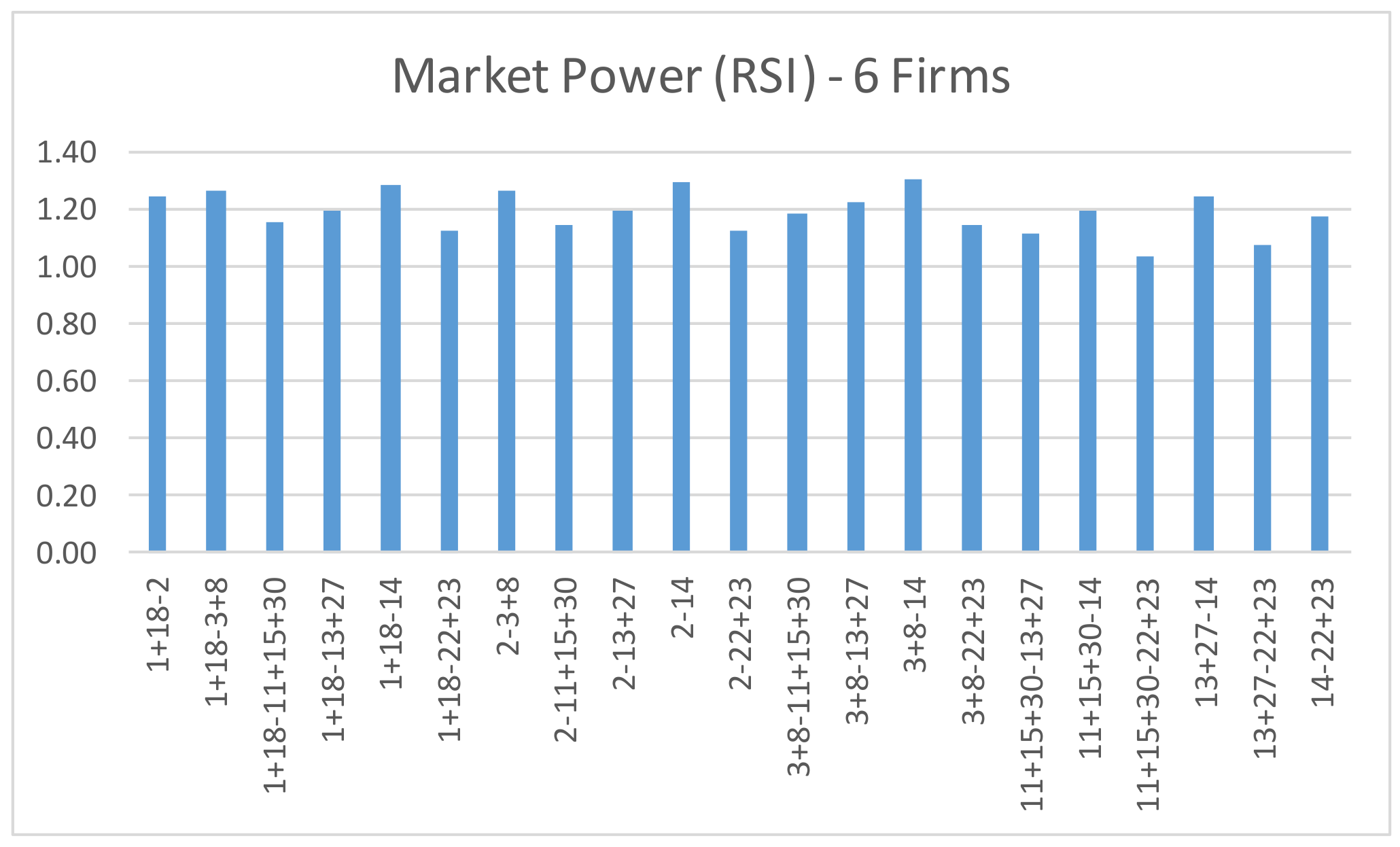
It should be noted that each cascading optimization in the study calculates various factors such as nodal price, nodal demand, nodal supply, nodal consumer surplus, nodal producer surplus, and power flow for each market configuration. However, for the purpose of our analysis, we primarily focus on the Residual Supply Index (RSI) calculation for each market setting. Specifically, we select the highest RSI value among all possible market settings as our main point of emphasis. This algorithm’s overarching goal is to achieve a competitive market structure that maximizes welfare while addressing any issues with generation capacity and reserve margin. Policymakers and market designers can follow this four-step process.

The methodology used in this study is a single-shot game methodology in which generating firms submit fixed supply functions to the ISO while taking into account their competitors’ bid functions. This is used for a single bidding period, and once all firms have submitted bids, the ISO clears the market, resulting in a market-clearing price. This price is determined by the ISO based on the market’s generation and transmission network structure, as well as the balance of supply and demand for electricity. The ISO pays the bus nodal price to all generating firms based on the amount of electricity sold to the pool in this model, and consumers pay the ISO the electricity price based on the active power load received.

3.1. Nodal Pricing and DC Power Transmission System

The concept of nodal pricing, as established by [34,35], is a fundamental theory used to determine optimal electricity prices that achieve welfare maximization under specific constraints. In this research, we perform a nodal pricing analysis based on Optimal Power Flow (OPF) and a marginal cost calculation at each node. The authors of ref. [36] incorporated transmission constraints and optimized electricity prices as a dual value in the program’s implementation of nodal pricing in the England and Wales market. The authors of ref. [27] expanded on this implementation by accounting for transmission losses in the optimal power flow (OPF) in order to apply nodal pricing in the same market. However, in this study, transmission losses are assumed to be minimal, and the load flow formulation is approximated into the DC load flow. The equilibrium structure is then used to calculate the Nash equilibrium for specific bid functions and the electricity network [37].

Kirchhoff’s law is a fundamental principle that governs power flow in power systems. The vector sum of the currents at any node in a circuit must be zero. This law governs all electrical circuits, including power grids. Kirchhoff’s law can be restated in terms of power flow in a grid as the vector sum of a node’s input and output being equal to the electricity injection at that node. This means that the power flow through any node in the system must be balanced, with the power flowing in equaling the power flowing out. Kirchhoff’s law must be followed to ensure the stability and reliability of the power system, as any deviation from this principle can cause power flow imbalances and potential power outages. To ensure the accuracy and stability of our power flow calculations, we use Kirchhoff’s law as a fundamental principle in our bottom-up electricity market model in this study.

We assume that bus i is the sending node and j is the receiving node, connected by transmission line ij. $V_m$ is the voltage magnitude, $V_{\mathsf{\theta }}$ is the voltage angle, and $\mathsf{\theta }$ is the phase angle. $G_{ij}$ and $B_{ij}$, respectively, are conductance and susceptance of transmission line ij. The AC power flow from bus i to j is defined as $P_{ij}\left(AC\right)$:

$$P_{ij}\left(AC\right)=V_m{V}_{\mathsf{\theta }}\left[G_{ij}\cos \left({\mathsf{\theta }}_i-{\mathsf{\theta }}_j\right)+B_{ij}\sin \left({\mathsf{\theta }}_i-{\mathsf{\theta }}_j\right)\right]-V_m^2{G}_{ij}$$

(1)

If $P_{ij}$ is positive, then the power is flowing from bus i to bus j, and vice versa.

Using the AC power flow equation, the DC power flow $P_{ij}\left(DC\right)$ assumes that voltage magnitudes bus i and j equal to 1 p.u. (per unit) and $\left({\mathsf{\theta }}_i-{\mathsf{\theta }}_j\right)<\frac{2\pi }{9}$, which implies that $\cos \left({\mathsf{\theta }}_i-{\mathsf{\theta }}_j\right)\approx 1$ and $\sin \left({\mathsf{\theta }}_i-{\mathsf{\theta }}_j\right)\approx \left({\mathsf{\theta }}_i-{\mathsf{\theta }}_j\right)$ for a normal operating condition in the power system.

$$P_{ij}\left(DC\right)=B_{ij}\left({\mathsf{\theta }}_i-{\mathsf{\theta }}_j\right)$$

(2)

In power system theory, the susceptance $B_{ij}$ is the imaginary part of admittance $Y_{ij}$ and could be denoted as $\frac{1}{X_{ij}}$ where $X_{ij}$ is the reactance of the transmission lines. Thus, the DC power flow could be stated as:

$$\left({\mathsf{\theta }}_i-{\mathsf{\theta }}_j\right)=X_{ij}{P}_{ij}\left(DC\right)$$

(3)

We assume a power setting with m transmission lines and n nodes. $X$ is a vector of reactance (m × m). $P_F$ is a vector of DC power flow (m × 1). M is the node–branch incidence matrix for the angle phase vector matrix (n − 1 × m) excluding the reference node (slack bus), i.e., the node with phase angle is zero. P is the power injection matrix (n − 1 × 1). B is the susceptance matrix. PTDF is the power transfer distribution factor. The DC power flow vector equation could be expressed in a matrix form as PTDF vector multiplies the power injection vector:

$$\begin{gathered} PTDF=X^{-1}{M}^T{B}^{-1} \\ {M}^T\mathsf{\theta }=X{P}_F \\ {P}_F=X^{-1}{M}^T\mathsf{\theta } \\ P=M{P}_F=M{X}^{-1}{M}^T\mathsf{\theta }=B\mathsf{\theta } \\ {P}_F=X^{-1}{M}^T{B}^{-1}P=PTDF P \\ {P}_F={\displaystyle \sum }_{i}PTDF\left( q_{si}-q_{di}\right) \end{gathered}$$

(4)

The power injection at node n is calculated using the DC power flow assumption as the difference between power generation production $q_{Si}$ and consumer demand $q_{li}$. As a result, the transmission line’s power flow can be represented as a linear function of PTDF and $q_{si}-q_{di}$.

3.2. Supply and Demand

The GenCo generates electricity based on the actual cost of the generator, while the consumer provides demand functions that represent the amount of electricity consumed. The demand function is the derivative of the benefit function, while the marginal cost function is the derivative of the total cost function. The consumer utility function is an inverse quadratic function as follows:

$$U{D}_i\left(q_{di}\right)=a_i{q}_{di}-b_i{q}_{di}{}^2;i=1,\dots , I$$

(5)

The load demand coefficient and active load demand at node i are represented by $a_i$, $b_i$, and $q_{di}$, respectively. The coefficient $a_i$ is a positive value, and $I$ indicates the number of consumers.

The demand function’s slope is negative, and it follows a linear form in the inverse.

$$p_i\left(q_{di}\right)=a_i-b_i{q}_{di};i=1,\dots ,I$$

(6)

Total generation cost $T{C}_i\left(q_{si}\right)$ consists of fixed ($f_i$) and variable cost $C_i\left(q_{si}\right)$

$$T{C}_i\left(q_{si}\right)=f_i+c_i{q}_{si}+\frac{1}{2}{d}_i{q}_{si}{}^2;i=1,\dots ,I$$

(7)

$$C_i\left(q_{si}\right)=c_i{q}_{si}+\frac{1}{2}{d}_i{q}_{si}{}^2; i=1,\dots ,I$$

(8)

$$U{D}_i\left(q_{li}\right)=c_i{q}_{li}-\frac{1}{2}{d}_i{q}_{li}{}^2;i=1,\dots , I$$

(9)

The bid or marginal cost function $M{C}_i\left(q_{si}\right)$ of a generating firm is represented as a linear function because a constant marginal cost does not fully capture the true cost of generation in the power sector. We defined $c_i$ as the intercept of the marginal cost, while $d_i$ was the slope of the marginal cost which reflected the true cost of the Genco.

$$M{C}_i\left(q_{si}\right)=c_i+d_i{q}_{si}; i=1,\dots ,I$$

(10)

Consumer surplus is defined as the net benefit of consumers. The total consumer surplus is computed by adding the individual consumer surpluses based on the price. The consumer surplus in each region is determined by a variety of factors, including the structure of the power network, the location of generators and consumers, and transmission constraints. Let $D_i\left(p_i\right)$ represent consumer i’s electricity demand at price $\left(p_i\right)$. The consumer surplus for the inverse linear demand function is expressed as follows:

$$C{S}_i\left(p_i\right)=\frac{1}{2}\left(a_i-p_i\right)D_i\left(p_i\right); i=1,\dots ,I$$

(11)

The producer surplus is the profit earned by a generator from selling electricity to the power pool and can be expressed as $P{S}_i\left(p_i\right)$.

$$P{S}_i\left(p_i\right)=\frac{1}{2}\left(p_i-c_i\right)q_{si}\left(p_i\right); i=1,\dots ,I$$

(12)

3.3. ISO Problem in Nodal Pricing

The system operator balances electricity supply and demand using a mechanism known as the balancing mechanism. The ISO’s goal is to maximize total welfare, denoted by ${\pi }_i \left(p\right)$, by selecting a single price for each bus I (1, …, I) in the network while taking the network’s limits (generation and transmission) into account as both inequality and equality constraints. Let $P_i\left(q_{di}\right)$ represent the benefit from electricity consumption, $M{C}_i\left(q_{si}\right)$ represent the total cost of generators at node $i$, $q_{si}$ represent the active load supply from the generator at bus $i$, and ${\overline{q}}_{si}$ represent the available capacity of the generator at node $i$. The problem of maximizing ISO welfare can be expressed as follows:

$$\begin{gathered} \begin{array}{c}max\\ q_{di}\end{array}\left({\displaystyle \sum }_i{P}_i\left(q_{di}\right)q_{di}-{\displaystyle \sum }_{i}M{C}_i\left(q_{si}\right)\right) \\ \mathrm{Subject} \mathrm{to}/\mathrm{constraints}: \\ \mathrm{Electricity} \mathrm{demand} \mathrm{balance} {{\displaystyle \sum }}_i{q}_{si}-{{\displaystyle \sum }}_i{q}_{di}=0 \\ \mathrm{Transmission} \mathrm{constraint} {{\displaystyle \sum }}_l\mathit{PTDF}\left({ q}_{si}-{ q}_{di}\right)\le T_l,-T_l \le {{\displaystyle \sum }}_l\mathit{PTDF}\left({ q}_{si}-{ q}_{di}\right) \\ \mathrm{Generation} \mathrm{constraint} q_{si}\le {\overline{q}}_{si} \\ \mathrm{Non}-\mathrm{negativity} q_{di}>0,q_{si}>0 \end{gathered}$$

(13)

3.4. Cournot Equilibrium Determination

We assume each node has a unique inverse linear demand function and the total demand function is defined as:

$$P\left(Q\right)=\alpha -\beta Q$$

(14)

where Q is the total demand for a particular interconnected power system and P is the Cournot equilibrium price.

In a competitive electricity market, generating firms make decisions on the amount of electricity they wish to produce and sell, based on market conditions and their own costs. This output decision, in turn, affects the market price level through the inverse demand relationship. In a single-shot game, firms assume that their rivals’ outputs are constant and use this information to calculate their own profit function, which is the difference between their benefit function and total cost function. The role of the independent system operator (ISO) is to ensure that this profit function is maximized for all players, taking into account the constraints imposed by the power network. In a Cournot equilibrium, the profit function for each firm (i) is given by a specific mathematical equation that takes into account the output decisions and costs of all firms in the market.

$${\pi }_i=\left(\alpha -\beta \left({\displaystyle \sum }_{i=1}^{i=I}{q}_i\right)\right)q_i-\left(f_i+c_i{q}_i+\frac{1}{2}{d}_i{q}_i{}^2\right)$$

(15)

The above profit function is in quadratic form and concave. Hence, the derivative solution for ISO profit maximization is easy to calculate.

$$\frac{d{\pi }_i}{d{Q}_i}=\alpha -\beta \left({\displaystyle \sum }_{i=1}^{i=I}{q}_i\right)-\beta q_i-\left(c_i+d_i{q}_i\right)$$

(16)

Taking the function’s derivative with respect to each node and setting it to zero yields a matrix equation with the variable subject to the total demand and cost function coefficients. The array’s size is determined by the number of participants in the electricity network.

When the derivative function is set to zero in each node, a matrix equation with $q_i$ as the subject variable and subject to the total demand and cost function coefficient is obtained. The array’s size is determined by the number of participants in the electricity network.

$$\begin{gathered} \left[\begin{array}{ccccc}-2\beta -d_1& -\beta & \dots & -\beta & -\beta \\ -\beta & -2\beta -d_2& \dots & -\beta & -\beta \\ \dots & \dots & \dots & \dots & \dots \\ -\beta & -\beta & \dots & -2\beta -d_{I-1}& -\beta \\ -\beta & -\beta & \dots & -\beta & -2\beta -d_I\end{array}\right]\left[\begin{array}{c}{q}_1\\ q_2\\ \dots \\ q_{I-1}\\ q_I\end{array}\right]=\left[\begin{array}{c}{c}_1-\alpha \\ c_2-\alpha \\ \dots \\ c_{I-1}-\alpha \\ c_I-\alpha \end{array}\right] \\ \left[\begin{array}{c}{q}_1\\ q_2\\ \dots \\ q_{I-1}\\ q_I\end{array}\right]={\left[\begin{array}{ccccc}2\beta +d_1& \beta & \dots & \beta & \beta \\ \beta & 2\beta +d_2& \dots & \beta & \beta \\ \dots & \dots & \dots & \dots & \dots \\ \beta & \beta & \dots & 2\beta +d_{I-1}& \beta \\ \beta & \beta & \dots & \beta & 2\beta +d_I\end{array}\right]}^{-1}\left[\begin{array}{c}\alpha -c_1\\ \alpha -c_2\\ \dots \\ \alpha -c_{I-1}\\ \alpha -c_I\end{array}\right] \end{gathered}$$

(17)

The FOC profit maximization has diagonal function $2\beta +d_i$ with $0<\beta <1$ and $0<d_i<1$; therefore, the coefficient of the matrix is positive and will give a unique solution for each $q_i$.

The object variable $q_i$ is the Cournot best response function in the network and could be defined as $q_i^{*}.$

$$q_i^{*}=\frac{\left(\alpha -c_i\right)-\left(\beta {{\displaystyle \sum }}_{i\ne j}^j{q}_j\right)}{2\beta +d_I}$$

(18)

In a case where the generating firms are symmetric, i.e., produce electricity in a uniform marginal cost, $c_i$ and $d_i$ coefficients are equivalent for all firms.

The power system is composed of numerous subnetworks in the actual power system topology, with each node representing a single load serving entity (LSE) and one or more power plant technologies. Each power plant technology, such as the base, intermediate, and peaking power plants, has a distinct linear marginal cost that reflects its distinct generation characteristics. The power system’s power plant technology mix can be classified based on the power plant’s ability to ramp-up and ramp-down to adjust to fluctuations in LSE aggregate electricity demand. Peak-load power plants have high ramping rates, low fuel costs, and relatively short construction times, whereas base-load power plants have low ramping rates, low fuel costs, and relatively short construction times.

When a GenCo operates multiple power plants, it behaves similarly to a monopolist with multiple plants, with the marginal cost of each plant determining the cost of generating electricity. When two power plants merge, their marginal cost functions are added horizontally. The efficiency constant used in the merger process is 1, which means that the GenCo’s efficiency before and after the merger is the same ($e_{pre-merger}=e_{post-merger}$).

To describe the system with two power plants that have a linear marginal cost $m{c}_1=c_1+d_1{q}_1$ and $m{c}_2=c_2+d_2{q}_2$, the combining marginal cost is $m{c}_{12}$, where $c_{12}=\left[\frac{c_1{d}_2+c_2{d}_1}{d_1+d_2}\right]$ and $d_{12}=\left[\frac{d_1{d}_2}{d_1+d_2}\right]$. The merger of the power plants results in changes to both the original marginal costs $m{c}_i$ and the supplier capacity k where $k_{12}=k_1+k_2$. Note that for uniform power plant capacity, the combined generation capacity is the maximum supplier capacity $k_{max}=k_{12}$.

The application of forward contract in this study is following the work by the authors of [23]. The producers could supply electricity in the forward market by determining a definite quantity as contract coverage, and then bid in the spot market. The system operator clears the market according to the Cournot game. Based on [23], we assume two players $x$ and $y$ with inverse demand function $q\left(z\right)=\left(a-z\right)$. The cost functions are $c\left(x\right)=bx$ and $d\left(y\right)=by$ with forward contracts $f$ and $g$, respectively. The profit functions in the Cournot equilibrium for $x$ and $y$ with a constant marginal cost and forward sales are ${\pi }_x=\left(a-x-y\right)\left(x-f\right)-bx)$ and ${\pi }_y=\left(a-x-y\right)\left(y-g\right)-by$. Solving FOC for both equations above leads to reaction function $x\left(y\right)=\frac{a-b+f-y}{2}$. The quantity’s Nash equilibriums are $x=\frac{a-b+2f-g}{3}$ and $y=\frac{a-b+2g-f}{3}$, while the Cournot price is $q=\frac{a-b-f-g}{3}$.

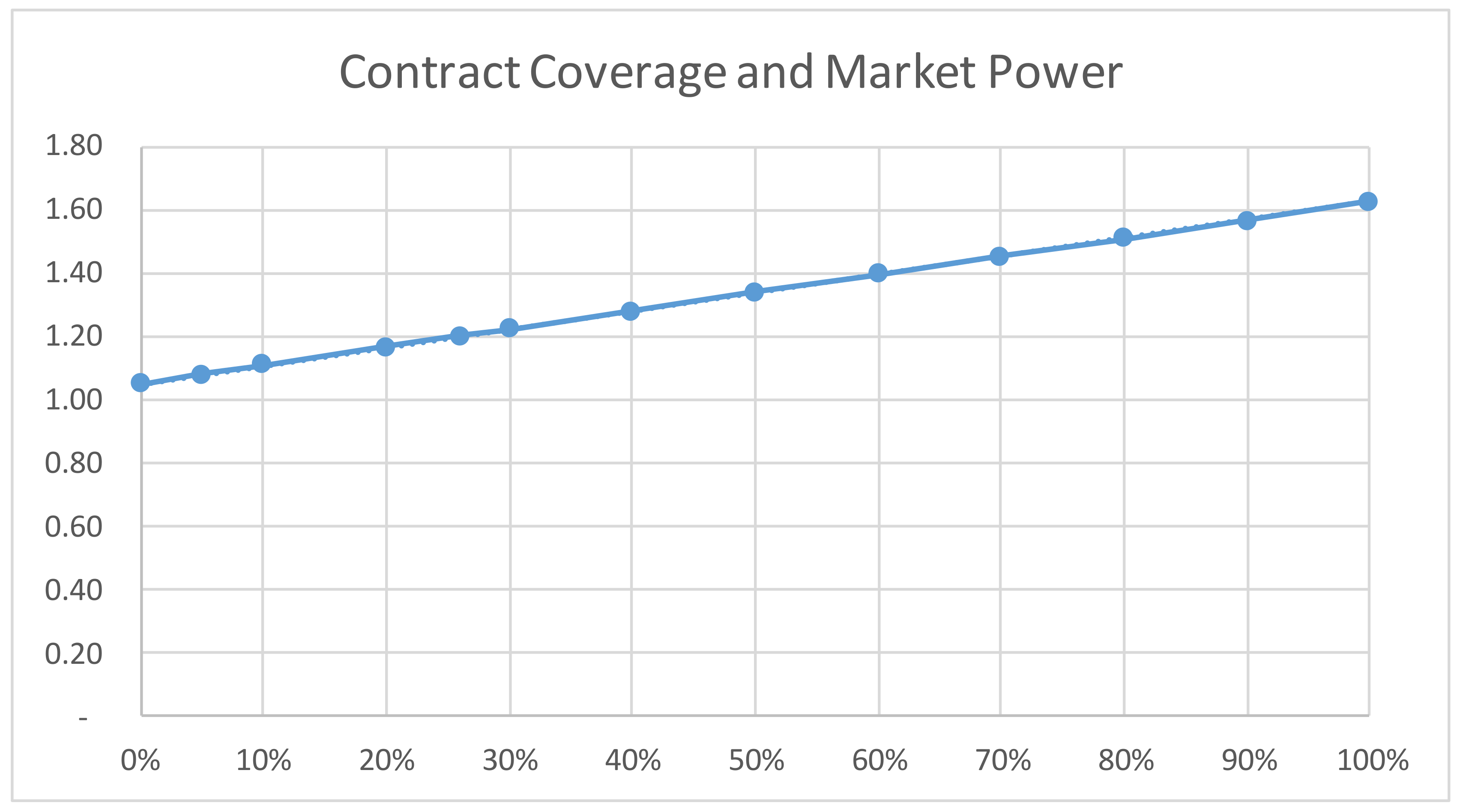
The authors of ref. [21] conducted a forward contract study using the RSI and proving that the RSI is suitable for a competition analysis and has an ability to determine the potential of generators to raise prices considering contracts and non-price-responsive supplies. Incorporating the forward contract, the RSI formula is $r_i=\frac{k^T-k_i}{Q}$, where $k^T$ is the total installed capacity, Q is the total demand equilibrium, and $k_{i }$ is the relevant capacity (capacity—forward contract). Based on this equation, the forward contract reduces the GenCo’s relevant capacity. Therefore, the contract mitigates the market power by increasing the residual supply faced by the market.

4. Case Study and Numerical Results

4.1. Case Study: Modified IEEE 30 Bus

In this study, we use a modified IEEE 30 bus power system to gain insights into power system analysis and economics. The system comprises 132 and 33 kV transmission lines with a combination of single, parallel, and phi line configurations. This test system is composed of five power producer nodes, twelve load serving entities nodes, eight power producer–load serving entities nodes, and the remaining nodes are null nodes with zero supply and demand. We have assumed the presence of 13 power plants located at nodes (1, 2, 3, 8, 11, 13, 14, 15, 18, 22, 23, 27, 30). To determine the optimal ownership structure and the mix of successor companies, we model the IEEE 30 bus electricity system into three types of power plant technology: base, intermediate, and peak power plants. As seen in Figure 1, base-load power plants are located at nodes 2, 11, 14, 22, and 23, and are represented in green. Intermediate power plants are located at nodes 1, 13, 18, and 27 and are represented in blue. Lastly, peak power plants are located at nodes 3, 8, 15, and 30 and are represented in yellow. The marginal cost is a linear function, as can be seen in

Table 1. Marginal cost function.

Type	PP	${\mathit{c}}_{\mathit{i}}$	${\mathit{d}}_{\mathit{i}}$
Base	Coal PP	30	0.1
Intermediate	Gas	35	0.15
Peaking	Diesel	40	0.2

.

The IEEE 30 bus power system is distinguished by its radial structure, with power flowing from the source to the loads via a single path, as well as its interconnection with other power systems. These characteristics must be taken into account when analyzing the behavior of the power system and optimizing its performance. The arrangement of components in the power system, including generators, transmission lines, transformers, and loads, is one of the unique features of the power system topology. The topology of the IEEE 30 nodes system includes the specific types of components used, the system layout and design, and the specific operating conditions under which the system operates. The system, for example, includes a mix of base-, intermediate-, and peaking-load power plants, and the transmission lines vary in length and capacity. These characteristics influence the behavior of the power system and must be considered when analyzing its performance.

The IEEE 30 bus power system is chosen as the test system in this study due to its widespread acceptance in the power system community and well-documented properties. The modified IEEE 30 bus power system used in this study includes a variety of transmission line configurations, load serving entities, and power producer nodes. It consists of a mix of base, intermediate, and peak power plants, which are the most common types of power plants in the electricity industry. We can gain valuable insights into the optimal ownership structure and the mix of successor companies by modeling this system, which can help policymakers and market designers create a competitive electricity market structure. Additionally, by using a well-known and well-documented system, we can ensure the replicability and generalizability of our results. Overall, the use of the IEEE 30 bus power system in this study is justified as it provides a realistic and well-documented test bed for a power system analysis and economics.

The marginal cost function for each type of power plant, which includes base-load PP, intermediate PP, and peaking PP, is displayed in Table 1. $c_i$ and $d_i$ represent the intercepet and slope of the marginal cost function, respectively.

Table 2. Load and installed capacity (MW).

n	${\mathit{k}}_{\mathit{i}} \left(\mathbf{MW}\right)$	${\mathit{q}}_{\mathit{d}\mathit{i}} \left(\mathbf{MW}\right)$	n	${\mathit{k}}_{\mathit{i}} \left(\mathbf{MW}\right)$	${\mathit{q}}_{\mathit{d}\mathit{i}} \left(\mathbf{MW}\right)$
1	100	10	16	0	9
2	200	0	17	0	0
3	50	20	18	100	35
4	0	0	19	0	17
5	0	85	20	0	60
6	0	0	21	0	34
7	0	50	22	150	0
8	130	25	23	150	85
9	0	0	24	0	9
10	0	190	25	0	9
11	120	0	26	0	0
12	0	50	27	120	0
13	120	20	28	0	27
14	160	50	29	0	35
15	100	50	30	30	0

lists the nodal information, including the generation capacity and load demand for each node in MW. The total demand in the system is 1530 MW, which is equivalent to the total supply. The demand and marginal cost functions are based on real-world data and have been calibrated to align with actual nodal and aggregated demand and supply. The nodal demand in this test system is characterized by an inelastic demand curve, which remains unchanged for the Cournot case study. In addition, we use transmission line capacity data as specified in

Table 3. Transmission line characteristics in IEEE 30 bus power system.

$\mathbf{From} \mathit{i}$	$\mathbf{to} \mathit{j}$	${\mathit{X}}_{\mathit{i}\mathit{j}} (\mathbf{p}.\mathbf{u})$	${\mathit{T}}_{\mathit{l}} \left(\mathbf{MW}\right)$	$\mathbf{From} \mathit{i}$	$\mathbf{to} \mathit{j}$	${\mathit{X}}_{\mathit{i}\mathit{j}} (\mathbf{p}.\mathbf{u})$	${\mathit{T}}_{\mathit{l}} \left(\mathbf{MW}\right)$
1	2	0.06	130	15	18	0.22	100
1	3	0.19	130	18	19	0.13	100
2	4	0.17	65	19	20	0.07	132
3	4	0.04	130	10	20	0.21	64
2	5	0.2	130	10	17	0.08	64
2	6	0.18	90	10	21	0.07	64
4	6	0.04	90	10	22	0.15	64
5	7	0.12	140	21	22	0.02	64
6	7	0.08	130	15	23	0.2	64
6	8	0.04	132	22	24	0.18	96
6	9	0.21	96	23	24	0.27	100
6	10	0.56	96	24	25	0.33	64
9	11	0.21	65	25	26	0.38	130
9	10	0.11	65	25	27	0.21	65
4	12	0.26	65	28	27	0.4	65
12	13	0.14	65	27	29	0.42	64
12	14	0.26	64	27	30	0.6	64
12	15	0.13	132	29	30	0.45	18
12	16	0.2	64	8	28	0.2	32
14	15	0.2	64	6	28	0.06	32
16	17	0.19	100

to accurately represent the transmission constraints in the system. This information is crucial for understanding the power flow dynamics and economic behavior of the market participants in the simulation.

4.2. Numerical Results

This section presents the results of a power system simulation that was conducted to explore the impact of different market structures on the overall performance of the system. We use the IEEE 30 bus power system model as the basis for our simulation and apply it to three different scenarios: (1) locational marginal pricing (LMP) with transmission constraints as a base case, (2) Cournot modeling, and (3) Cournot with forward contracts. The main objective of this numerical analysis is to determine the optimal mix and structure for each case study, the minimum number of players needed to create a competitive market, and the optimal contract coverage. To achieve this, we use a deterministic approach and provide ad-hoc configurations for each market structure. Through this simulation, we aim to gain valuable insights into the effects of different market structures on the performance of the power system and identify the most efficient and effective market design for ensuring a competitive and well-functioning electricity market.

4.2.1. Base Case: Nodal Pricing with Transmission Constraint

The load flow for the base case power system can be seen in Figure 2 below. As illustrated in the figure, congestion arises at lines 1–4, 2–9, 3–12 and 4–14, indicating that transmission constraints are limiting the ability of local power producers with low marginal costs in certain regions to transfer their cheap power to other areas. This results in market power, higher electricity prices, and lower welfare. Furthermore, in real power systems, these transmission bottlenecks can lead to forced system outages where the load flow exceeds its transfer limit and causes damage to the cables. This further enables power producers to exercise market power.

Table 4. Congested transmission lines IEEE 30 bus.

No	$\mathbf{From} \mathit{i}$	$\mathbf{To} \mathit{j}$	${\mathit{P}}_{\mathit{i}\mathit{j}}\left(\mathit{D}\mathit{C}\right) \left(\mathbf{MW}\right)$ Case 1: Perfect Competition
1	4	6	90
2	9	10	65
3	12	13	−65
4	14	15	64

below illustrates the four congested transmissions in the IEEE 30 bus power system, providing a clear picture of the transmission constraints that are impacting the power system.

The shift factor matrix, as shown in

Table 5. Shift factor matrix IEEE 30 test bus.

	1	2	3	4	5	6	7	8	9	10	11	12	13	14	15	16	17	18	19	20	21	22	23	24	25	26	27	28	29	30
1	0.662	−0.177	0.152	0.045	−0.092	−0.007	−0.041	−0.007	0.002	0.006	0.002	0.024	0.024	0.021	0.019	0.016	0.009	0.015	0.012	0.011	0.007	0.007	0.015	0.008	0.003	0.003	0.00E+00	−0.006	0.00E+00	0.00E+00
2	0.338	0.177	−0.152	−0.045	0.092	0.007	0.041	0.007	−0.002	−0.006	−0.002	−0.024	−0.024	−0.021	−0.019	−0.016	−0.009	−0.015	−0.012	−0.011	−0.007	−0.007	−0.015	−0.008	−0.003	−0.003	0.00E+00	0.006	−2.22E−16	0.00E+00
3	0.224	0.303	−0.024	−0.076	0.157	0.012	0.070	0.012	−0.003	−0.011	−0.003	−0.041	−0.041	−0.036	−0.033	−0.028	−0.016	−0.025	−0.021	−0.018	−0.012	−0.012	−0.025	−0.014	−0.006	−0.006	0.00E+00	0.011	0.00E+00	0.00E+00
4	0.338	0.177	0.848	−0.045	0.092	0.007	0.041	0.007	−0.002	−0.006	−0.002	−0.024	−0.024	−0.021	−0.019	−0.016	−0.009	−0.015	−0.012	−0.011	−0.007	−0.007	−0.015	−0.008	−0.003	−0.003	0.00E+00	0.006	0.00E+00	0.00E+00
5	0.136	0.161	0.055	0.038	−0.422	−0.006	−0.172	−0.006	0.002	0.005	0.002	0.020	0.020	0.018	0.016	0.014	0.008	0.012	0.010	0.009	0.006	0.006	0.012	0.007	0.003	0.003	4.44E−16	−0.005	0.00E+00	0.00E+00
6	0.302	0.358	0.122	0.084	0.173	−0.013	0.061	−0.013	0.003	0.012	0.003	0.044	0.044	0.040	0.036	0.031	0.018	0.028	0.023	0.020	0.013	0.013	0.027	0.016	0.006	0.006	4.44E−16	−0.012	0.00E+00	0.00E+00
7	0.404	0.326	0.650	0.701	0.109	−0.108	−0.021	−0.106	0.029	0.101	0.029	0.372	0.372	0.333	0.303	0.257	0.147	0.232	0.190	0.168	0.106	0.108	0.229	0.130	0.051	0.051	1.78E−15	−0.096	0.00E+00	0.00E+00
8	0.136	0.161	0.055	0.038	0.578	−0.006	−0.172	−0.006	0.002	0.005	0.002	0.020	0.020	0.018	0.016	0.014	0.008	0.012	0.010	0.009	0.006	0.006	0.012	0.007	0.003	0.003	0.00E+00	−0.005	2.22E−16	0.00E+00
9	−0.136	−0.161	−0.055	−0.038	−0.578	0.006	−0.828	0.006	−0.002	−0.005	−0.002	−0.020	−0.020	−0.018	−0.016	−0.014	−0.008	−0.012	−0.010	−0.009	−0.006	−0.006	−0.012	−0.007	−0.003	−0.003	0.00E+00	0.005	4.44E−16	0.00E+00
10	0.129	0.129	0.128	0.128	0.129	0.130	0.130	−0.736	0.117	0.110	0.117	0.113	0.113	0.110	0.108	0.112	0.110	0.109	0.109	0.109	0.105	0.104	0.098	0.085	0.033	0.033	1.78E−15	−0.063	0.00E+00	0.00E+00
11	0.126	0.128	0.118	0.116	0.135	0.142	0.140	0.140	−0.474	−0.273	−0.474	−0.082	−0.082	−0.103	−0.119	−0.164	−0.241	−0.173	−0.205	−0.222	−0.255	−0.249	−0.141	−0.172	−0.067	−0.067	−1.78E−15	0.127	−9.99E−16	0.00E+00
12	0.072	0.073	0.067	0.067	0.077	0.081	0.080	0.080	−0.075	−0.156	−0.075	−0.047	−0.047	−0.059	−0.068	−0.094	−0.138	−0.099	−0.117	−0.127	−0.145	−0.142	−0.081	−0.098	−0.038	−0.038	−9.99E−16	0.073	−5.55E−16	0.00E+00
13	0.0E+00	0.0E+00	4.4E−16	8.9E−16	0.0E+00	0.0E+00	4.4E−16	0.0E+00	−4.4E−16	0.0E+00	−1.0E+00	4.4E−16	4.4E−16	0.0E+00	4.4E−16	4.4E−16	0.0E+00	4.4E−16	0.0E+00	0.0E+00	−4.4E−16	0.0E+00	0.0E+00	0.0E+00	0.0E+00	0.0E+00	2.2E−16	4.4E−16	1.1E−16	0.0E+00
14	0.126	0.128	0.118	0.116	0.135	0.142	0.140	0.140	0.526	−0.273	0.526	−0.082	−0.082	−0.103	−0.119	−0.164	−0.241	−0.173	−0.205	−0.222	−0.255	−0.249	−0.141	−0.172	−0.067	−0.067	−1.33E−15	0.127	−1.11E−15	0.00E+00
15	0.159	0.154	0.174	0.177	0.140	0.127	0.132	0.124	−0.034	−0.118	−0.034	−0.437	−0.437	−0.390	−0.355	−0.301	−0.172	−0.272	−0.223	−0.197	−0.124	−0.126	−0.269	−0.153	−0.059	−0.059	2.22E−16	0.113	1.11E−16	0.00E+00
16	8.88E−16	0.00E+00	1.78E−15	0.00E+00	1.78E−15	0.00E+00	0.00E+00	0.00E+00	8.88E−16	1.78E−15	8.88E−16	8.88E−16	−1.00E+00	1.78E−15	8.88E−16	1.78E−15	8.88E−16	0.00E+00	−8.88E−16	1.78E−15	1.78E−15	0.00E+00	8.88E−16	8.88E−16	1.33E−15	4.44E−16	4.44E−16	8.88E−16	0.00E+00	0.00E+00
17	0.028	0.027	0.030	0.030	0.026	0.024	0.025	0.024	0.007	−0.001	0.007	0.076	0.076	−0.463	−0.109	0.043	0.012	−0.072	−0.049	−0.037	−0.006	−0.008	−0.075	−0.029	−0.011	−0.011	6.66E−16	0.021	−1.11E−16	0.00E+00
18	0.099	0.097	0.105	0.106	0.091	0.085	0.087	0.084	0.026	−0.004	0.026	0.270	0.270	−0.101	−0.387	0.153	0.042	−0.253	−0.174	−0.132	−0.023	−0.028	−0.266	−0.102	−0.040	−0.040	−4.44E−16	0.076	−6.66E−16	0.00E+00
19	0.032	0.030	0.039	0.041	0.024	0.018	0.020	0.017	−0.068	−0.112	−0.068	0.217	0.217	0.174	0.141	−0.498	−0.226	0.053	0.000	−0.028	−0.096	−0.091	0.072	−0.021	−0.008	−0.008	−1.11E−15	0.016	−6.66E−16	0.00E+00
20	0.028	0.027	0.030	0.030	0.026	0.024	0.025	0.024	0.007	−0.001	0.007	0.076	0.076	0.537	−0.109	0.043	0.012	−0.072	−0.049	−0.037	−0.006	−0.008	−0.075	−0.029	−0.011	−0.011	−1.33E−15	0.021	−2.22E−16	0.00E+00
21	0.032	0.030	0.039	0.041	0.024	0.018	0.020	0.017	−0.068	−0.112	−0.068	0.217	0.217	0.174	0.141	0.502	−0.226	0.053	0.000	−0.028	−0.096	−0.091	0.072	−0.021	−0.008	−0.008	−1.55E−15	0.016	−6.66E−16	0.00E+00
22	0.004	0.003	0.008	0.008	−0.001	−0.004	−0.003	−0.004	−0.056	−0.083	−0.056	0.106	0.106	0.151	0.185	0.026	−0.051	−0.559	−0.408	−0.327	−0.067	−0.062	0.109	0.005	0.002	0.002	−1.11E−15	−0.004	−4.44E−16	0.00E+00
23	0.004	0.003	0.008	0.008	−0.001	−0.004	−0.003	−0.004	−0.056	−0.083	−0.056	0.106	0.106	0.151	0.185	0.026	−0.051	0.441	−0.408	−0.327	−0.067	−0.062	0.109	0.005	0.002	0.002	−4.44E−16	−0.004	0.00E+00	0.00E+00
24	0.004	0.003	0.008	0.008	−0.001	−0.004	−0.003	−0.004	−0.056	−0.083	−0.056	0.106	0.106	0.151	0.185	0.026	−0.051	0.441	0.592	−0.327	−0.067	−0.062	0.109	0.005	0.002	0.002	0.00E+00	−0.004	−4.44E−16	0.00E+00
25	−0.004	−0.003	−0.008	−0.008	0.001	0.004	0.003	0.004	0.056	0.083	0.056	−0.106	−0.106	−0.151	−0.185	−0.026	0.051	−0.441	−0.592	−0.673	0.067	0.062	−0.109	−0.005	−0.002	−0.002	1.11E−15	0.004	6.66E−16	0.00E+00
26	−0.032	−0.030	−0.039	−0.041	−0.024	−0.018	−0.020	−0.017	0.068	0.112	0.068	−0.217	−0.217	−0.174	−0.141	−0.502	−0.774	−0.053	0.000	0.028	0.096	0.091	−0.072	0.021	0.008	0.008	8.88E−16	−0.016	8.88E−16	0.00E+00
27	0.146	0.147	0.145	0.145	0.147	0.148	0.148	0.146	0.205	0.234	0.205	0.121	0.121	0.102	0.087	0.169	0.215	0.139	0.169	0.185	−0.435	−0.340	−0.026	−0.179	−0.069	−0.069	−2.66E−15	0.132	−1.33E−15	0.00E+00
28	0.088	0.088	0.087	0.087	0.088	0.089	0.089	0.087	0.123	0.141	0.123	0.073	0.073	0.061	0.052	0.102	0.129	0.083	0.101	0.111	−0.127	−0.204	−0.015	−0.107	−0.042	−0.042	−8.88E−16	0.079	−4.44E−16	0.00E+00
29	0.146	0.147	0.145	0.145	0.147	0.148	0.148	0.146	0.205	0.234	0.205	0.121	0.121	0.102	0.087	0.169	0.215	0.139	0.169	0.185	0.565	−0.340	−0.026	−0.179	−0.069	−0.069	0.00E+00	0.132	0.00E+00	0.00E+00
30	0.123	0.121	0.127	0.128	0.117	0.113	0.115	0.111	0.090	0.077	0.090	0.240	0.240	0.284	0.319	0.171	0.105	0.234	0.185	0.158	0.038	0.026	−0.450	−0.137	−0.053	−0.053	−2.22E−16	0.101	−2.22E−16	0.00E+00
31	0.234	0.234	0.232	0.232	0.236	0.237	0.237	0.233	0.328	0.375	0.328	0.194	0.194	0.163	0.140	0.271	0.344	0.222	0.271	0.297	0.438	0.456	−0.041	−0.286	−0.111	−0.111	2.22E−15	0.212	1.33E−15	0.00E+00
32	0.123	0.121	0.127	0.128	0.117	0.113	0.115	0.111	0.090	0.077	0.090	0.240	0.240	0.284	0.319	0.171	0.105	0.234	0.185	0.158	0.038	0.026	0.550	−0.137	−0.053	−0.053	−6.66E−16	0.101	−2.22E−16	0.00E+00
33	0.357	0.356	0.360	0.360	0.353	0.351	0.352	0.344	0.417	0.452	0.417	0.434	0.434	0.448	0.458	0.442	0.449	0.456	0.455	0.454	0.476	0.482	0.509	0.577	−0.164	−0.164	1.11E−15	0.313	6.66E−16	0.00E+00
34	0.00E+00	0.00E+00	0.00E+00	0.00E+00	0.00E+00	0.00E+00	0.00E+00	0.00E+00	0.00E+00	−4.44E−16	0.00E+00	0.00E+00	0.00E+00	0.00E+00	−2.22E−16	0.00E+00	0.00E+00	2.22E−16	2.22E−16	−2.22E−16	0.00E+00	0.00E+00	0.00E+00	−2.22E−16	0.00E+00	−1.00E+00	−1.11E−16	0.00E+00	0.00E+00	0.00E+00
35	0.357	0.356	0.360	0.360	0.353	0.351	0.352	0.344	0.417	0.452	0.417	0.434	0.434	0.448	0.458	0.442	0.449	0.456	0.455	0.454	0.476	0.482	0.509	0.577	0.836	0.836	1.11E−15	0.313	5.55E−16	0.00E+00
36	−0.643	−0.644	−0.640	−0.640	−0.647	−0.649	−0.648	−0.656	−0.583	−0.548	−0.583	−0.566	−0.566	−0.552	−0.542	−0.558	−0.551	−0.544	−0.545	−0.546	−0.524	−0.518	−0.491	−0.423	−0.164	−0.164	−7.77E−16	−0.687	−4.44E−16	0.00E+00
37	0.399	0.399	0.399	0.399	0.399	0.399	0.399	0.399	0.399	0.399	0.399	0.399	0.399	0.399	0.399	0.399	0.399	0.399	0.399	0.399	0.399	0.399	0.399	0.399	0.399	0.399	3.99E−01	0.399	−3.22E−01	0.00E+00
38	0.601	0.601	0.601	0.601	0.601	0.601	0.601	0.601	0.601	0.601	0.601	0.601	0.601	0.601	0.601	0.601	0.601	0.601	0.601	0.601	0.601	0.601	0.601	0.601	0.601	0.601	6.01E−01	0.601	3.22E−01	0.00E+00
39	0.429	0.429	0.429	0.429	0.429	0.429	0.429	0.429	0.429	0.429	0.429	0.429	0.429	0.429	0.429	0.429	0.429	0.429	0.429	0.429	0.429	0.429	0.429	0.429	0.429	0.429	4.29E−01	0.429	7.30E−01	0.00E+00
40	0.129	0.129	0.128	0.128	0.129	0.130	0.130	0.264	0.117	0.110	0.117	0.113	0.113	0.110	0.108	0.112	0.110	0.109	0.109	0.109	0.105	0.104	0.098	0.085	0.033	0.033	−2.22E−16	−0.063	0.00E+00	0.00E+00
41	0.515	0.515	0.512	0.512	0.517	0.520	0.519	0.391	0.466	0.438	0.466	0.453	0.453	0.442	0.433	0.447	0.441	0.435	0.436	0.436	0.420	0.414	0.393	0.338	0.131	0.131	0.00E+00	−0.250	0.00E+00	0.00E+00

, is a crucial tool in determining the optimal load flow for each transmission line in the base case scenario. This matrix represents the proportion of the load on each line that is shifted to other lines in order to alleviate transmission congestion and improve overall system performance. By analyzing the shift factors, it is possible to identify which lines are the most congested and in need of additional capacity or upgrades. Furthermore, the shift factors can be used to determine the most cost-effective solutions for addressing transmission constraints, such as building new transmission lines or upgrading existing ones. Additionally, this information can also be used to inform pricing mechanisms and market design, as it can help to identify which generators are most affected by transmission constraints and therefore may be able to exercise more market power. Overall, the shift factor matrix is an essential tool for understanding and improving the performance of power systems in a competitive market environment.

The pre-model market configuration consists of 13 firms with a total capacity of 1530 MW. Through the application of a merger analysis in the model, we have determined the optimal market structure for 12 players as can be seen in

Table 6. Optimal market structure and configuration.

n Firm	$\mathit{r}$	Combination
12	1.526	15 Merge 30
11	1.521	3 Merge 11
10	1.497	1 Merge 18
9	1.418	13 Merge 27
8	1.387	8 Merge 15 + 30
7	1.324	14 Merge 22
6	1.294	3 + 11 Merge 23
5	1.185	1 + 18 Merge 2
4	1.043	8 + 15 + 30 Merge 13 + 27

and Figure 3. This optimal structure is achieved when the power plant in node 15 is combined or merged with the power plant in node 30. The merger results in a Residual Supply Index (RSI) of 1.526, indicating that the combined firm’s market power is reduced, and competition is enhanced. A merger analysis is a common approach used in antitrust policy to assess the potential effects of a merger on competition in a market. By analyzing the market structure and the impact of a merger on the concentration of market power, regulators can make informed decisions on whether to approve or reject a proposed merger. In this case, the merger of the two power plants in nodes 15 and 30 is deemed to be optimal as it results in a more competitive market, with reduced market power and increased welfare for consumers.

The use of the Residual Supply Index (RSI) in a merger analysis is a key approach to identifying the optimal market structure for a competitive electricity market. By analyzing the combination of generation technology and the installed capacity of power producers post-merger, this approach allows for the creation of competition between different generation technologies within a firm and the spreading of large, pivotal power plants among multiple competitive players. The RSI was first introduced in the California electricity market by [1], and traditionally a threshold of 120% is used to determine a reasonable competitive market. In this study, a six-player configuration with an RSI of 1.294 is identified as the minimum number of players needed to create a competitive market, while a configuration with five players has an RSI of less than 1.2, indicating the potential for market power to be exercised. Figure 4, Figure 5, Figure 6, Figure 7, Figure 8, Figure 9, Figure 10, Figure 11 and Figure 12 display all of the possible configurations resulting from the merger.

4.2.2. Second Case: Cournot Model

Figure 13, Figure 14, Figure 15, Figure 16, Figure 17, Figure 18, Figure 19, Figure 20 and Figure 21 display all the possible configurations resulting from the merger in the Cournot assumption. In this Cournot case study, the simulation results in a slightly different optimal market structure compared to the base case scenario, as can be seen in Figure 22 and

Table 7. Cournot case study: optimal market structure.

n Firm	$\mathit{r}$	Combination
12	1.573	15 Merge 30
11	1.562	3 Merge 8
10	1.541	1 Merge 18
9	1.477	13 Merge 27
8	1.432	11 Merge 15 + 30
7	1.383	22 Merge 23
6	1.311	3 + 8 Merge 14
5	1.224	1 + 18 Merge 2
4	1.051	13 + 27 Merge 22 + 23

. The first merger step taken by the model is similar to the base case scenario, where two peaking power plants at nodes 15 and 30 are combined, resulting in a Residual Supply Index (RSI) of 1.573 in a 12-player market structure. However, the next merger steps taken to create the optimal market structure in eleven- to four-player configurations are different from the base case. This means that the minimum number of players needed to create a reasonably competitive electricity market is five players with an RSI of 1.224. Market configurations with player participation below five have the potential for market power exercise. The load flow for the locational marginal pricing (LMP) and Cournot modeling can be seen in

Table 8. DC load flow for PC and Cournot.

$\mathbf{From} \mathit{i}$	$\mathbf{to} \mathit{j}$	${\mathit{P}}_{\mathit{i}\mathit{j}}\left(\mathit{D}\mathit{C}\right) \left(\mathbf{MW}\right)$ Case 1: Perfect Competition	${\mathit{P}}_{\mathit{i}\mathit{j}}\left(\mathit{D}\mathit{C}\right) \left(\mathbf{MW}\right)$ Case 2: Cournot	${\mathit{T}}_{\mathit{l}} \left(\mathbf{MW}\right)$
1	2	27.0	20.0	130
1	3	37.6	23.6	130
2	4	43.0	25.7	65
3	4	44.8	26.9	130
2	5	79.8	66.9	130
2	6	60.6	33.1	90
4	6	90.0	39.6	90
5	7	−5.3	−17.7	140
6	7	55.0	66.4	130
6	8	3.3	0.3	132
6	9	43.1	−8.5	96
6	10	28.9	15.9	96
9	11	−21.9	−105.7	65
9	10	65.0	97.2	65
4	12	−2.2	13.0	65
12	13	−65.0	−32.1	65
12	14	−44.8	−24.1	64
12	15	9.0	0.2	132
12	16	48.5	19.8	64
14	15	64.0	31.4	64
16	17	39.6	11.7	100
15	18	15.8	31.0	100
18	19	80.8	46.1	100
19	20	63.8	25.4	132
10	20	−3.7	35.7	64
10	17	−39.6	−11.7	64
10	21	−30.0	−58.2	64
10	22	−22.5	−38.9	64
21	22	−64.0	−87.9	64
15	23	7.2	−20.1	64
22	24	−31.7	−21.1	96
23	24	32.3	5.5	100
24	25	−8.3	−17.3	64
25	26	0.0	0.0	130
25	27	−17.3	−20.4	65
28	27	1.1	26.6	65
27	29	21.8	12.8	64
27	30	4.8	−5.5	64
29	30	−14.0	−19.3	18
8	28	5.4	−0.5	32
6	28	20.3	−1.4	32

.

Table 8 presents the power transfer for each transmission cable in the LMP and Cournot case study. The table provides a detailed analysis of the power flow for each transmission line, including the congested lines identified in the base case scenario. The load flow for the LMP case study is calculated based on the transmission constraint and the optimal load flow for each transmission line, as determined by the shift factor matrix. On the other hand, the load flow for the Cournot case study is calculated based on the Cournot equilibrium, which takes into account the strategic behavior of the market players. The comparison between the two load flow results can provide insight into how different market structures and behaviors affect the power flow in the system. Additionally, the table also shows how the power transfer changes between the two scenarios, which can be used to identify the potential impact on market power and welfare.

4.2.3. Forward Contract in Cournot Model

Table 8 shows the power transfer for each transmission cable in the LMP and Cournot case study, with the addition of forward contract as a variable. The simulation results indicate that the Cournot model, when incorporating the forward contract as a portion of the installed capacity, is a suitable method for analyzing the market equilibrium. In order to ensure realistic data in the numerical simulation, we have avoided the conjured forward contract and instead calibrated contract coverage in the Cournot formula to determine the optimal contract coverage that can create a competitive market structure. The simulation results show that by using forward contract as an instrument, it is possible to create a competitive electricity market with a lower number of player participants, with the optimal market configuration resulting in an RSI of 1.005 with only four players. Furthermore, by calibrating the contract coverage, as can be seen in Figure 23 and Figure 24 and

Table 9. Contract coverage and RSI.

Scenario	Contract Coverage	$\mathit{r}$
1	0%	1.05
2	5%	1.08
3	10%	1.11
4	20%	1.17
5	26%	1.20
6	30%	1.22
7	40%	1.28
8	50%	1.34
9	60%	1.40
10	70%	1.45
11	80%	1.51
12	90%	1.57
13	100%	1.62

, we have determined that a minimum contract coverage of 26% is needed to increase the market power index to a competitive level.

5. Discussion

This study presents a preventive approach for optimizing the structure of electricity markets [11,13] by considering the use of forward contracts and using the IEEE 30 bus test system as a case study. The simulations demonstrate the ability to determine the optimal mix and structure of successor companies using a bottom-up merger approach. The use of the RSI as a measure of market power mitigation highlights the importance of a minimum number of players to create a reasonably competitive market. This study extends the application of forward contracts in Cournot models, as previously studied in [23,25], by incorporating the RSI as a tool to mitigate market power. It also extends the application of the RSI in the contract-Cournot study of [21] by applying the concept of forward contracts in a more complex market structure, represented by the IEEE 30 bus test system, and taking into account DC load flow.

The level of contract coverage in a competitive market plays a crucial role in maintaining competitiveness and reducing market power. The optimal level of contract coverage is determined by the model behavior and assumptions. According to the authors of [21], under a Cournot model with a constant marginal cost and linear demand schedule, the equilibrium level of contract coverage for each oligopolist is the same fraction of output. The level of forward contracting under a monopoly is 0%, increasing to 50% under a duopoly, and reaching up to 80% when there are five firms. It ultimately converges on full coverage with a sufficient number of companies. When power producers are fully contracted, the best strategy for them is to bid competitively in the spot market, as their bidding would not change the spot price, as per [24]. However, the authors of [25] have shown that the optimal contract coverage under the Cournot model in the German market is 50%, twice as much as in the SFE case.

In this study, we used a threshold of 1.2 for the Residual Supply Index (RSI) based on the experience of the California Independent System Operator (CAISO). Using Cournot modeling and a 120% RSI limit threshold, we found that a minimum of five players with a balanced mix of generation technology are needed to create a competitive market. Additionally, by using forward contracts as a tool to reduce market power, the market regulator could design a four-player configuration with an optimal contract coverage of 26%. It is important to note that the results of this simulation are subject to the assumptions and characteristics of the power system used, and that a dynamic calculation in a real-time power system could yield different results.

6. Conclusions

This study highlights the significance of utilizing an ex-ante analysis approach in the restructuring of electricity markets to ensure the creation of competitive successor companies. The goal of market restructuring should be to avoid the formation of market structures with firms possessing excessive market power. Poor market restructuring can lead to the emergence of a dominant GenCo, which can significantly increase market prices due to strategic behavior constrained by other GenCos. Conversely, successful market restructuring results in the formation of efficient and competitive successor companies. The use of preventive antitrust policies, as outlined in [38], plays a crucial role in preventing the formation of uncompetitive market structures by promoting wholesale configurations that foster competition and positive economic growth, while also preventing the abuse of dominant market power.

The main contribution of this paper is the development of an algorithm that can be used to optimize the structure of electricity markets in large power systems, providing a balanced mix of generation technologies for each GenCo. By using a bottom-up merger approach and incorporating forward contracts, the algorithm is able to determine the optimal mix and structure of successor companies in the IEEE 30 bus test system. The results of the simulations show that the Cournot market setting (with five players) offers a lower number of participants compared to the perfect competition setting (with six players). This is consistent with the preference configuration observed in the UK electricity market. However, it is important to note that the equilibrium is affected by the specific characteristics of the power system and the market power index threshold used.

An antitrust analysis is crucial in understanding the factors that drive prices away from marginal cost, such as scarcity rent and market power exercises. Without the implementation of antitrust laws and policies, market players may have the ability to exercise their market power. By monitoring the strategic behavior of players, electricity market authorities, such as OFGEM in the UK, FTC in the US, and KPPU in Indonesia, can maximize customer welfare by reducing the exercise of market power ex-ante. However, guidelines should be efficient, clear, and easily understood by players to avoid any potential business distortions. Effective laws and policies are a fundamental aspect of the application of economics in the real world. The use of simple yet insightful research tools is essential to achieve a comprehensive understanding of the electricity market.

While this study provides useful insights into mitigating market power in electricity markets through the use of forward contracts, some limitations should be noted. For starters, the proposed algorithm is based on a simplified model that does not take into account all of the complexities and nuances found in real-world electricity markets. Furthermore, the study only focuses on the IEEE 30 bus test case, which may not be representative of other electricity markets. Finally, the study is based on hypothetical forward contract data and does not include real-world data, which may limit the findings’ generalizability.

Future research could focus on incorporating real forward contract data into the algorithm to address these limitations. This would entail gathering and analyzing data on forward contracts in the electricity market, and then using this information to validate and improve the proposed algorithm. Such an approach would provide a more accurate reflection of market conditions and could provide valuable insights into the effectiveness of using forward contracts as a tool for market power mitigation. This study could also be expanded to include a broader range of electricity markets and investigate how the proposed algorithm performs under various scenarios and conditions.