Article

Integrating Survival Analysis with Bayesian Statistics to Forecast the Remaining Useful Life of a Centrifugal Pump Conditional to Multiple Fault Types

Swanson School of Engineering, University of Pittsburgh, Pittsburgh, PA 15260, USA
*
Author to whom correspondence should be addressed.
Energies 2023, 16(9), 3707; https://doi.org/10.3390/en16093707
Submission received: 14 March 2023 / Revised: 14 April 2023 / Accepted: 24 April 2023 / Published: 26 April 2023
(This article belongs to the Special Issue Forecasting Techniques for Power Systems with Machine Learning)

Abstract

:
To improve the viability of nuclear power plants, there is a need to reduce their operational costs. Operational costs account for a significant portion of a plant’s yearly budget, due to their scheduled-based maintenance approach. In order to reduce these costs, proactive methods are required that estimate and forecast the state of a machine in real time to optimize maintenance schedules. In this research, we use Bayesian networks to develop a framework that can forecast the remaining useful life of a centrifugal pump. To do so, we integrate survival analysis with Bayesian statistics to forecast the health of the pump conditional to its current state. We complete our research by successfully using the Bayesian network on a case study. This solution provides an informed probabilistic viewpoint of the pumping system for the purpose of predictive maintenance.

1. Introduction

In this article, we develop a machine health forecasting system for nuclear power plants (NPPs). Nuclear plants have scheduled maintenance outages at regular intervals. When a machine starts developing faults and stops operation, it requires repair or replacement. If the timeline of machine repair does not fall within the scheduled outages, the NPP needs to have an unplanned outage to inspect the machine, causing NPPs to lose potential revenue [1]. Even during planned outages, the maintenance process can be conservative and time-consuming, which can potentially increase operational costs [2]. In order to reduce these costs, a proactive condition monitoring approach is needed that improves operations and maintenance (O&M) using advancements in data analytics.
Condition monitoring is the process of estimating the health of a machine based on available parameter data, such as sensor measurements. Analyzing different parameters provides a range of information about developing faults and inefficiencies in the machinery. Condition monitoring is composed of three parts: monitoring, diagnosis, and forecasting. Monitoring observes a component, device or process and sends an alert when failure occurs. Diagnosis determines the root cause of failure which can be addressed by performing informed maintenance. Forecasting provides an estimate of the remaining useful life (RUL) of a machine and its components.
Deep learning methods have been used in RUL prediction of machines because of their ability to automatically map the relationship between raw data and machine life [3,4,5,6,7,8]. These methods are capable of revealing the underlying correlations between machine phenomenon and its reason. Therefore, they can be advantageous over physics-based or model-based approaches when the analyzed system becomes very complex. However, these approaches usually require a lot of raw data for training the network. They are also inherently “black box” in nature. Their internal logic can be unexplainable, which can hinder their potential to be deployed to a power plant and used by operators.
Probabilistic RUL estimation has been considered for machines due to its potential to be integrated into a larger decision-making framework [9,10,11,12]. These methods incorporate data driven machine learning with dynamic models to quantify prediction uncertainty. The uncertainty information is then used for decision making or to improve prediction results. These approaches are useful in decision making due to their probabilistic results, but the RUL predictions are not conditional to the current state of the machine. There is a need to account for the effect of different faults on the RUL because each fault degrades the machine in a unique manner.
Knowing the cause of degradation will directly improve O&M by removing the need for manual trial and error [13]. If we know what caused the failure, we can directly repair that specific defect. Knowing the cause of failure also has impacts on the supply chain by allowing the affected parts to be ordered well in advance. Therefore, a more comprehensive picture of the pumping system is required. An updated model would map system parameters to different faults, and their probability of occurrence would alter the RUL appropriately.
By performing this research, we establish the advantages of probabilistic uncertainty that can be leveraged by decision-makers. We demonstrate how to combine survival analysis with Bayesian statistics to conditionally update a machine’s RUL. Finally, we provide a condition monitoring solution to optimize O&M for NPPs, and by extension, other industrial plants.

2. Background

In order to develop a probabilistic forecasting tool, we integrate survival analysis with Bayesian networks. This allows us to create survival models for various modes of operation and relate them to the current state of the pump using conditional probabilities.

2.1. Bayesian Networks

Bayesian networks are probabilistic graphical models that represent a set of variables by their conditional probabilities. They allow for various types of information to be incorporated into a common probabilistic framework. The types of information include sensor data, uncertainties, expert opinion, and mathematical equations [14]. Bayesian networks allow us to analyze systems causally. This lets us describe complex and dynamic behavior without requiring elaborate physics-based models. The ability to describe the cause and effect relationship between different variables is a key advantage of Bayesian networks. They use statistical inference to estimate the occurrence of phenomenon based on observations or evidence. Inference is performed according to Bayes’ rule (Equation (1)), which describes the probability of an event conditional to some prior knowledge about the event. Bayes rule also allows us to update the event probability after obtaining new evidence.
P ( A | B ) = P ( B | A ) P ( A ) P ( B )
where
  • A and B are events and P ( B ) 0 ;
  • P ( A | B ) is the posterior probability; the probability of event A occurring if B is true;
  • P ( B | A ) is the likelihood; the probability of event B occurring if A is true;
  • P ( A ) is the prior; the probability of event A without having any knowledge of B;
  • P ( B ) is the marginal likelihood; the total probability of the evidence B.
Bayesian networks expand this idea to multiple variables that have a cause and effect relationship with each other. By identifying which variables influence others, conditional probabilities are propagated throughout the network. This lets us determine the probability of an event from the combined probability of its influencing evidence.
In this network,
Energies 16 03707 i001
variables A and B cause event C. The likelihood of event C occurring is affected by the likelihood of A and B both according to Equation (2).
P ( C ) = A , B P ( C | A , B ) P ( A ) P ( B )
This lets us determine the probability of C given our knowledge of A and B. We can also infer the probability of A or B given our knowledge of C [14].
Bayesian networks can be used to address the challenges of pump life forecasting. Estimating the RUL is not a trivial task since each fault degrades the pump at a different rate. The RUL is conditional on the type of fault occurring in the pump. This behavior can be modeled using Bayesian networks by developing conditional probability tables (CPT), given enough information about the system. Therefore, we diagnose the type of fault occurring in the pump first, then update the RUL accordingly.

2.2. Survival Analysis

Survival analysis is a collection of techniques to determine the expected amount of time before an events occurs, and this is accomplished by developing the survival function for the system. The survival function is the probability of an event occurring after a specified time. Mathematically, given that a machine fails before time T, with cumulative distribution F(T), and probability density f (T) = F’(T), the survival function S(t) is the probability that time T is after the current time t; i.e., S(t) is the probability that the device survives past time t.
S ( t ) = P ( T > t ) = t f ( τ ) d τ = 1 F ( t )
For our research, we define the life of the pump as the life of the impeller. The impeller faces constant dynamic forces that cause warping and chipping over its lifetime. Eventually, the impeller wears significantly and stops providing enough energy to the fluid to meet the required duty points. Abnormal operation exacerbates this process and degrades the impeller faster. After a certain threshold the worn impeller is no longer of use and the pump is said to have failed.
Survival analysis is suitable for machine forecasting because it can provide acceptable estimates even with incomplete data sets. This is beneficial since machine lifetime data is hard to obtain. To develop a prediction model, impeller lifetime data is desired. Synthetic lifetime data is generated to recreate the operation of an impeller rotating inside a pump. The dataset is used to train our predictive models to provide an estimate of the future impeller health.

3. Procedure

3.1. Pump System Specifications

The feedwater pumps in an NPP are chosen as the machine of choice for our analysis. Feedwater pumps are a crucial part of the energy generation process [15,16]. They are also usually very expensive, and improper maintenance can cost a lot of money.
A feedwater system typically contains pumps installed in a parallel with common suction and discharge headers, and are usually high-pressure centrifugal type. The piping for feedwater systems includes suction and discharge control valves that automatically open or close depending on the steam generator supply requirements. The conditions of service for the selected feedwater pump are 0.38 m 3 s 1 (6000 gpm) at 8.96   M Pa (1300 psi). These conditions are common requirements for NPPs. To meet these demands, a single stage horizontal centrifugal pump is configured. The pumping system is shown in Figure 1, and the pump performance parameters are specified in Table 1.

3.2. Pump Fault Mechanisms

For condition monitoring, we choose three modes of operation: normal operation, cavitation, and bent shaft occurrence [17,18]. Normal operation is the ideal state of the pump and is used as a baseline to train our Bayesian network. Cavitation and a bent shaft are two of the most violent faults that cause significant damage to a pump.
Fault diagnosis for centrifugal pumps is most commonly performed with vibration analysis [19,20,21,22,23,24]. Vibration analysis is the process of monitoring vibration signals within a machine to detect abnormal operating levels or patterns to evaluate its condition. A vibration signature consists of the amplitude and frequency of the signal. These signatures are unique for each pump fault detected, which in turn provide information about the health of the machine. Vibration is often at its lowest when the pump is running at its best efficiency point (BEP), and excessive vibration is a common indicator of a developing fault inside a pump. Cavitation causes random high frequency vibrations in the pump casing. A bent pump shaft will cause complex vibrations that require analysis in the frequency domain.

3.3. Data Generation

To create the Bayesian network, the conditional probabilities of each node pair need to be determined. In order to determine the CPTs, we use a data-driven approach. The normal and abnormal operation of the pump are simulated to generate synthetic sensor data. These datasets are used to compute the CPTs by applying a learning algorithm. The pump is modeled according to [25], with further modifications to add multiple abnormal operating conditions. This model consists of masses of different sizes that replicate the major parts of a pump. These masses are connected with springs and dampers to model the vibration characteristics of the various pump components.

3.4. Diagnosing Pump Faults

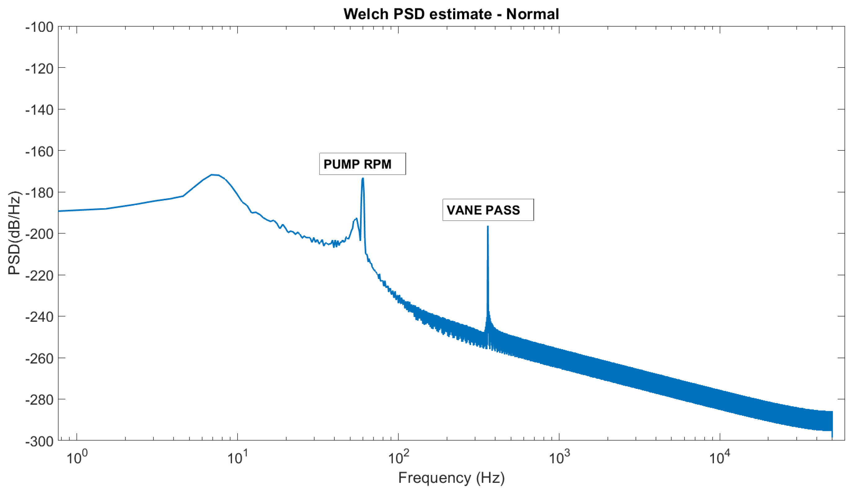
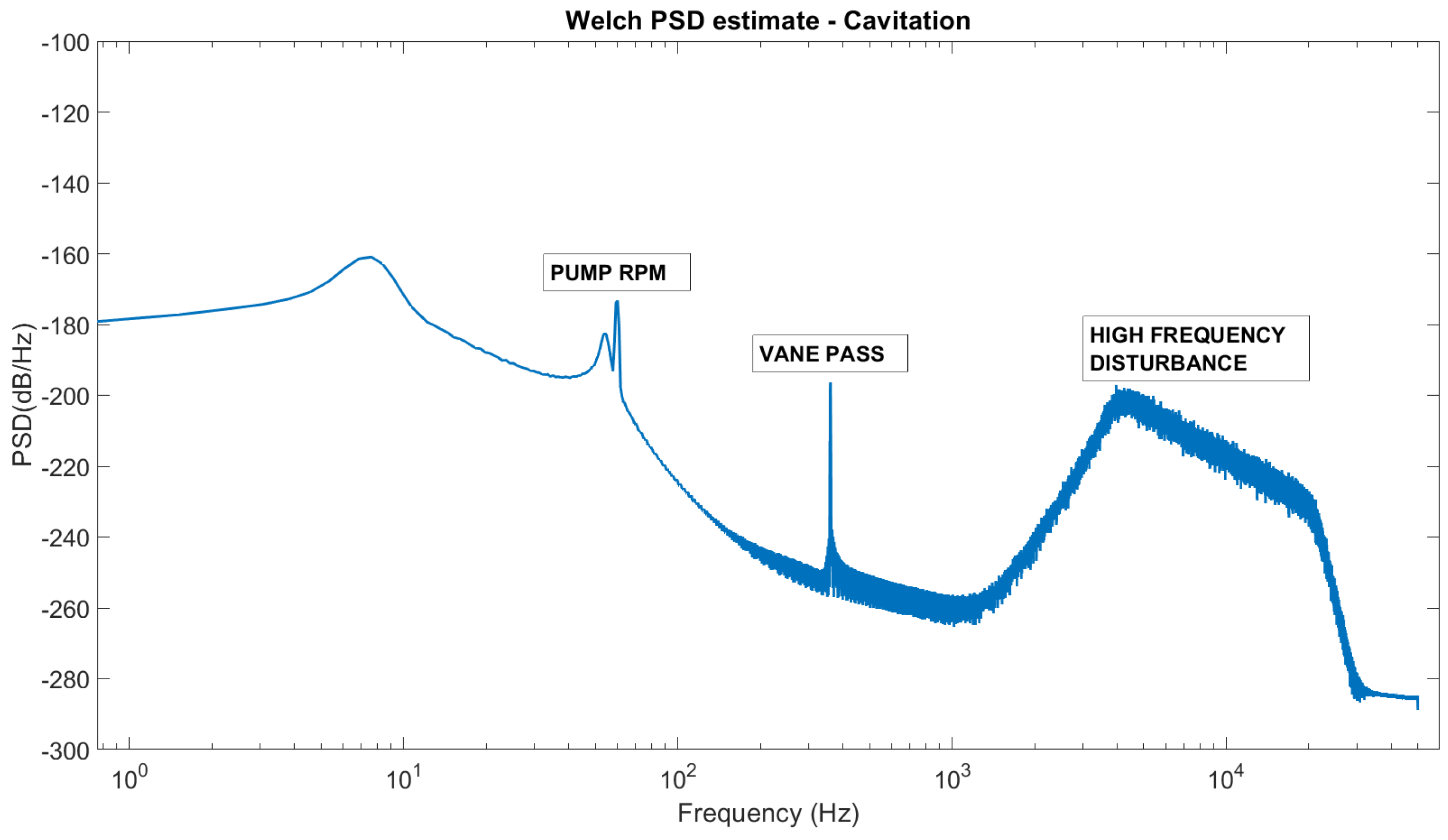
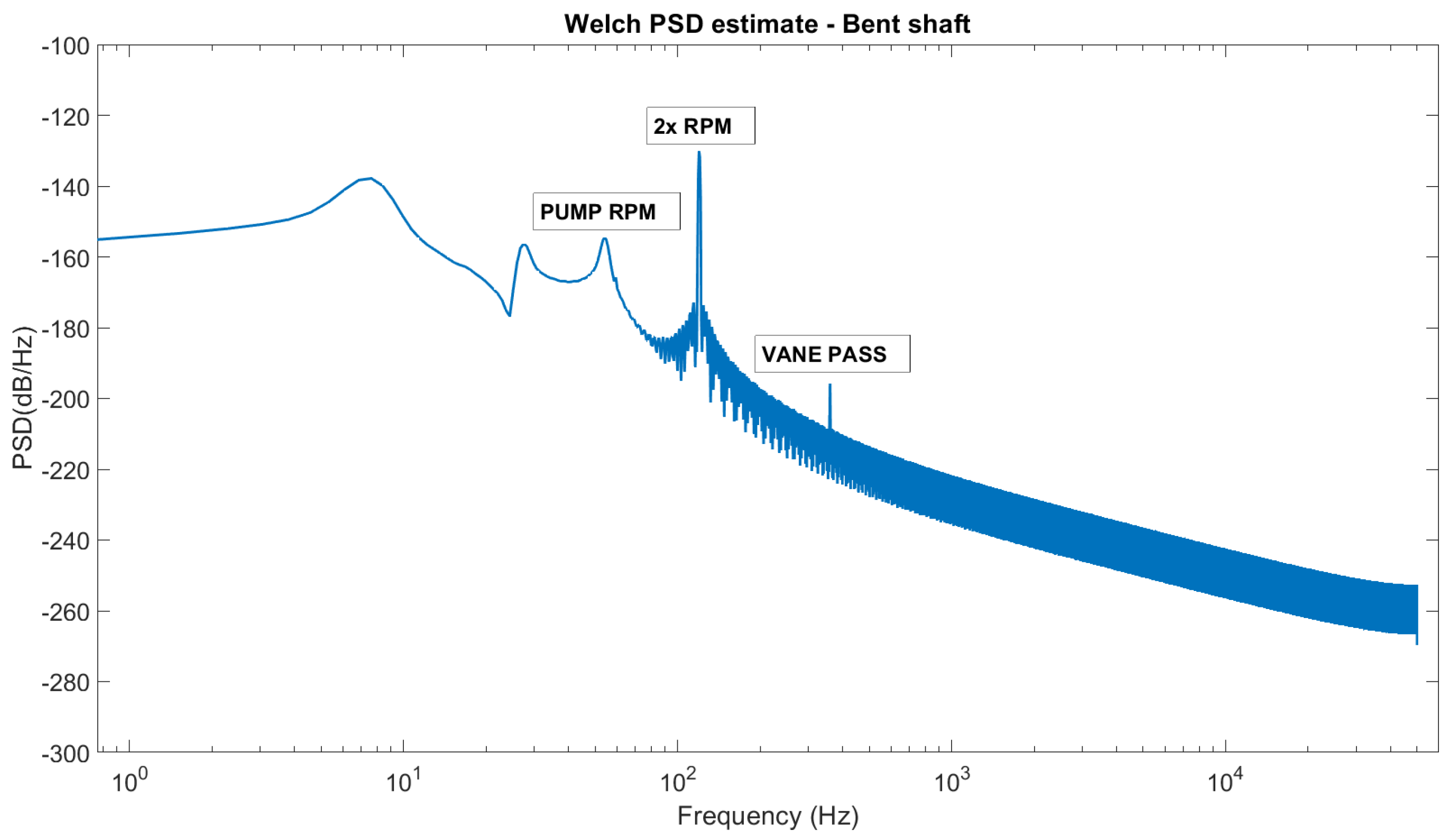
Once the pump model is created, we simulate its normal and abnormal operation to gather vibration data. Then we apply vibration analysis techniques on this data for the purpose of diagnosing the state of the pump. Each mode of operation has a unique vibration signature. For normal operation, we see peaks at the vane pass frequency (360 Hz) and the motor RPM (60 Hz) (Figure 2). Cavitation causes high amplitude disturbances in the spectra between 4 kHz and 20 kHz (Figure 3). A bent pump shaft causes high axial vibrations that result in a large amplitude spike at two-per-revolution (120 Hz) (Figure 4).
After performing the preliminary vibration analysis in the frequency domain, the vibration measurements are then decomposed into three features:
1.
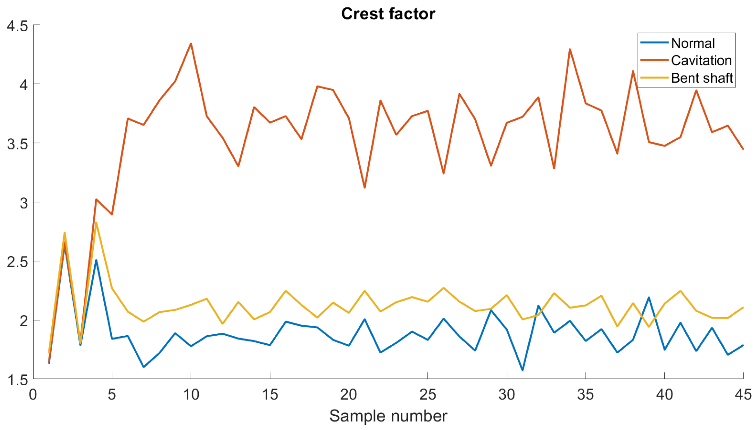
Crest factor: The crest factor is defined as the ratio of the peak value of a signal to its RMS value (Figure 5). A crest factor value of 1 indicates no peaks. Crest factor is calculated as
cf = x p x r m s
where x p is the maximum absolute value of the signal and x r m s is the root mean squared value of the signal.
2.
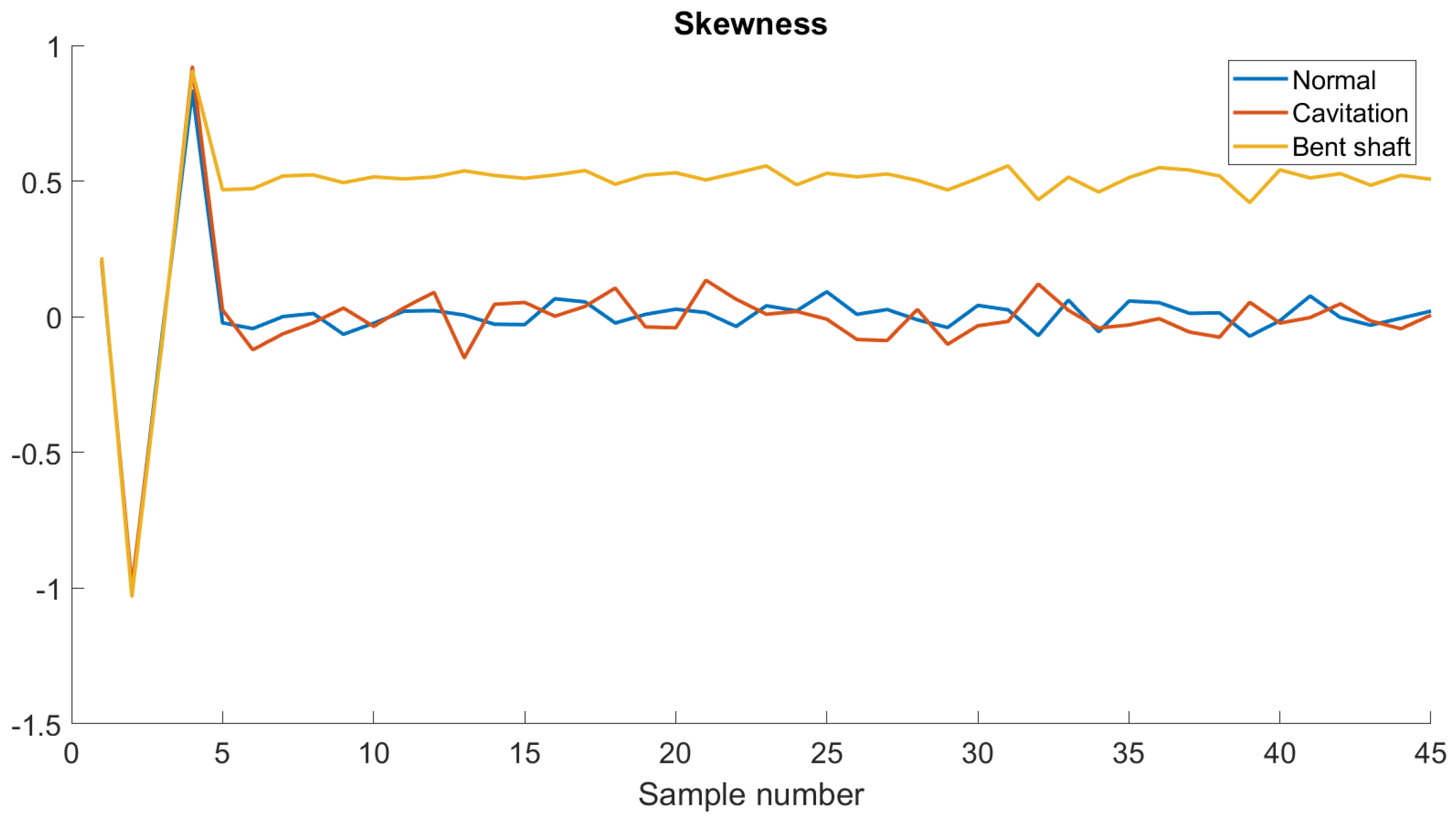
Skewness: Skewness is used to measure whether the signal is negatively or positively skewed (Figure 6). It is obtained from the mean value of the probability density function of the signal. Skewness is calculated as
s = 𝔼 { x μ 3 } σ 3
where μ is the mean of x, σ is the standard deviation of x, and 𝔼 { x } is the expected value of x.
3.
Kurtosis: Kurtosis is used to quantify the peakness of a signal (Figure 7). A higher kurtosis value corresponds to a signal with more peaks that are greater than three times the signal RMS. Kurtosis is calculated as
k = 𝔼 { x μ } 4 σ 4
These features are dimensionless normalized quantities. In order to analyze the machine state, these values need to be compared to an established baseline. In our research, we estimate the state of the pump by computing the features for normal operation and then comparing them to the values from cavitation and a bent shaft.
For the purpose of this article, we emphasize that the estimated state of the pump is probabilistic; i.e., the output of our diagnosis is the probability of normal operation, cavitation, or a bent shaft. Estimating the state of the pump probabilistically rather than deterministically is crucial because it allows the addition of uncertainty in condition monitoring-based decision-making.

3.5. Bayesian Network Creation for Forecasting

To develop a Bayesian network for condition monitoring, we use the GeNIe modeler and SMILE engine from BayesFusion [26]. The Bayesian network is developed using Figure 1 as reference. The evidence for the network are vibration measurements. The vibration information is added in the form of features. From these inputs, we can diagnose one of two faults, and forecast the pump’s health.
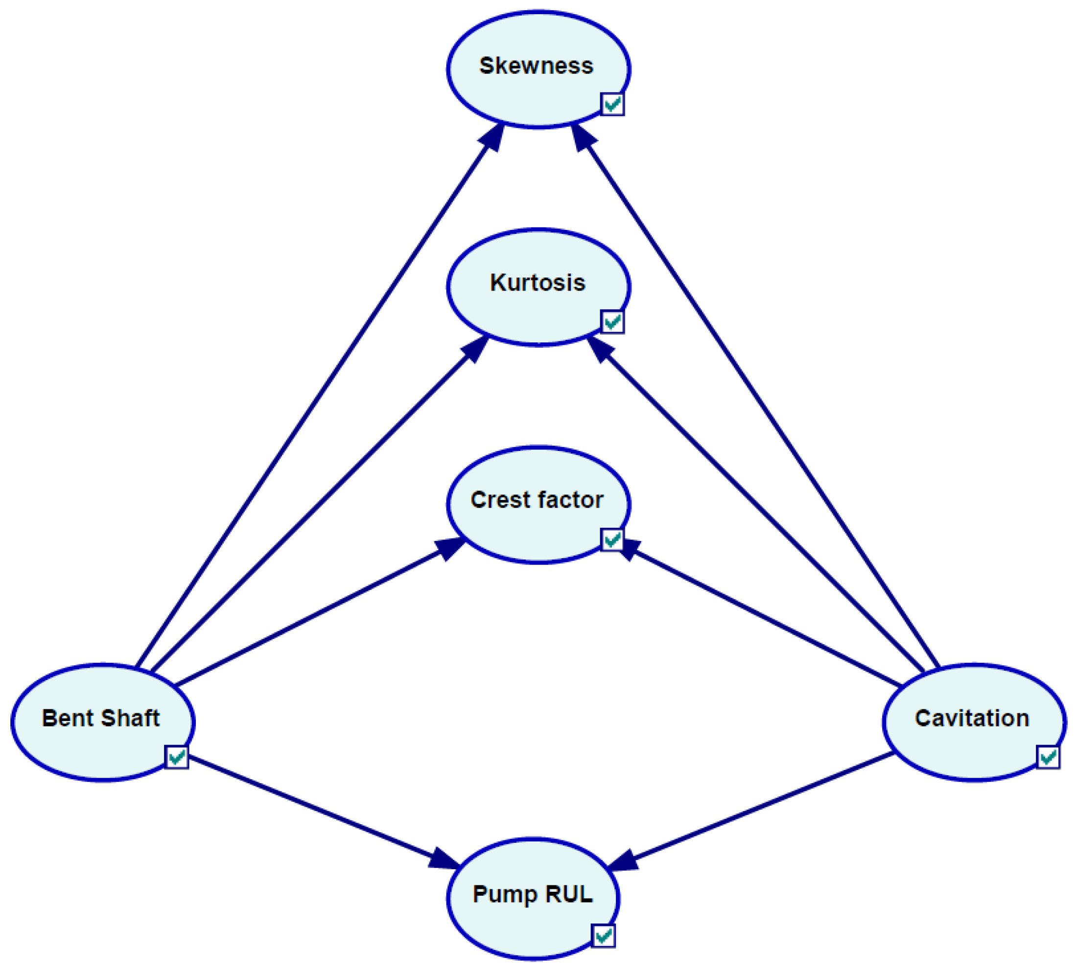
There is a unique combination of skewness, kurtosis, and crest factor values for each of the three simulated modes of operation. When the appropriate values are entered into these nodes as evidence, the Bayesian network can determine the current state of the pump. This relation is shown in Figure 8. The state of Bent Shaft and Cavitation directly affect the state of the Skewness, Kurtosis, and Crest factor. The state of the two faults also directly affect the Pump RUL.

3.6. Data Structuring for the Bayesian Network

In order to perform Bayesian inference using GeNIe and SMILE, the Bayesian network needs to contain discrete states. Discretization also allows parameter learning algorithms to create CPTs from data. Each node in the Bayesian network is discretized according to the states listed in Table 2, Table 3 and Table 4. The Cavitation and Bent Shaft nodes are discretized into binary states as either occurring or not occurring. This is because the occurrence of the fault is itself a binary phenomenon. However, the extent of a fault is not binary. For example, cavitation can cause high frequency disturbances at various amplitudes and a bent shaft can be askew by various degrees. The effect of the magnitude of fault is an open topic for future work. In this paper, we consider faults to be binary processes with constant magnitudes.
The CPTs for each node pair are created using a learning algorithm that is trained on the data generated previously. In order to create CPTs and perform parameter learning, we use the expectation-maximization (EM) algorithm [27].

3.7. Forecasting Health Using the Bayesian Network

To forecast pump RUL, we perform survival analysis on the pump lifetime data. The python package Lifelines is used for computing the survival functions [28]. The dataset contains run-to-failure data for a hundred pumps experiencing two different faults. The pumps begin operation with normal amounts of initial wear, but develop a fault over time. These faults persist through the time series until total failure.
A common preliminary method in survival analysis is to develop the Kaplan–Meier estimator, which computes the the Kaplan–Meier survival plot from data. It is defined as
S ^ ( t ) = t i < t n i d i n i
where d i is the number of failure events at time t i and n i is the number of machines that have survived up to time t i .
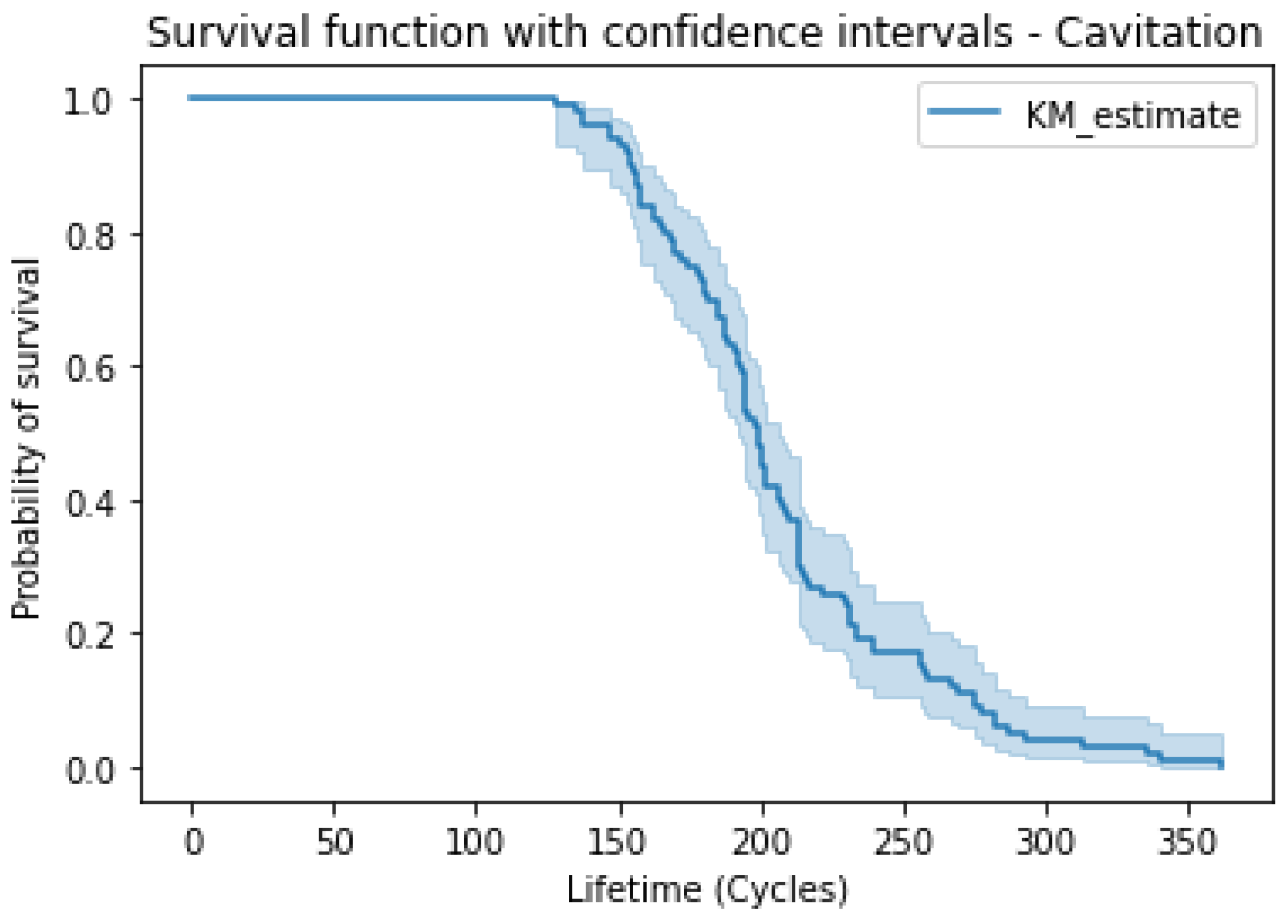
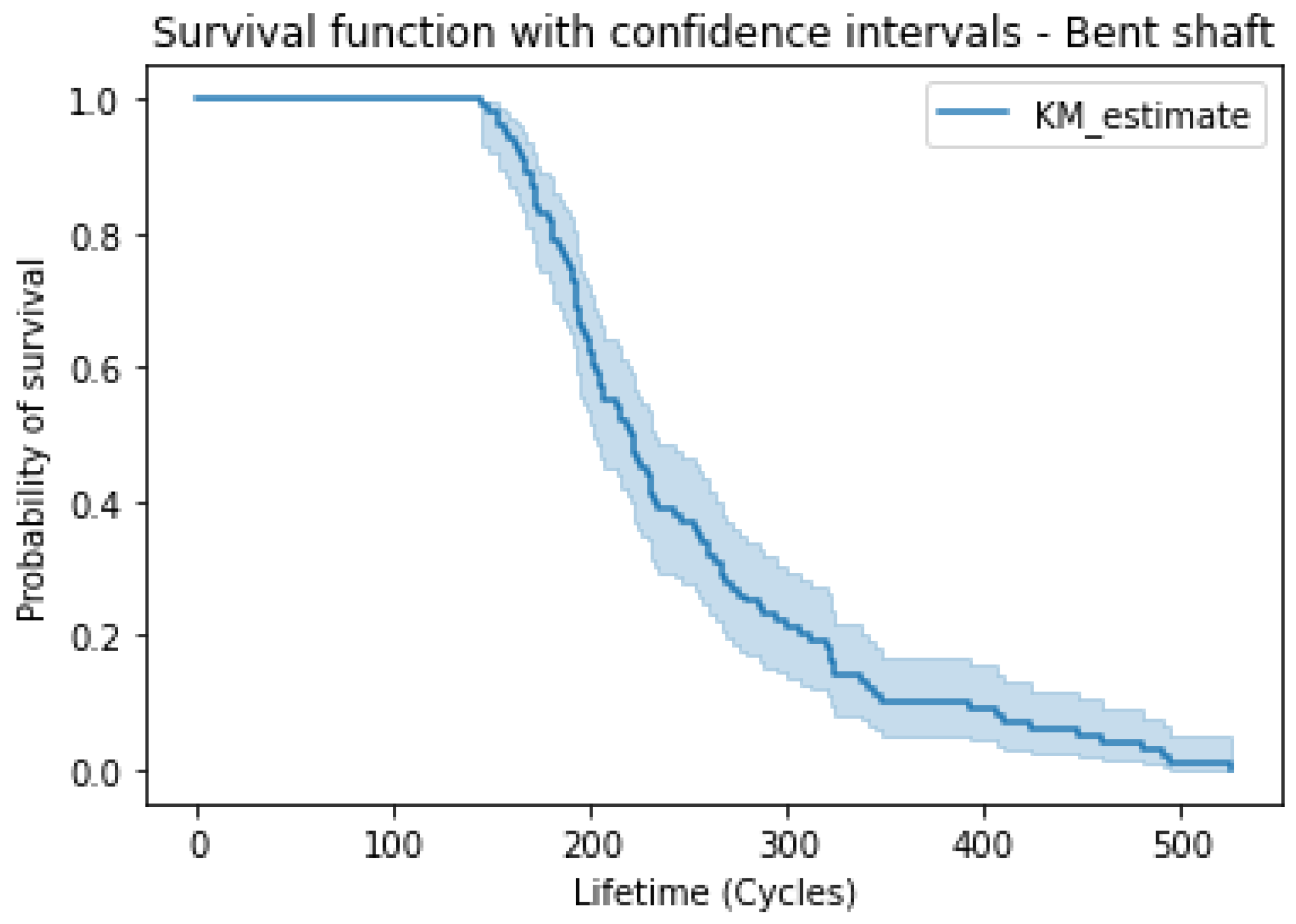
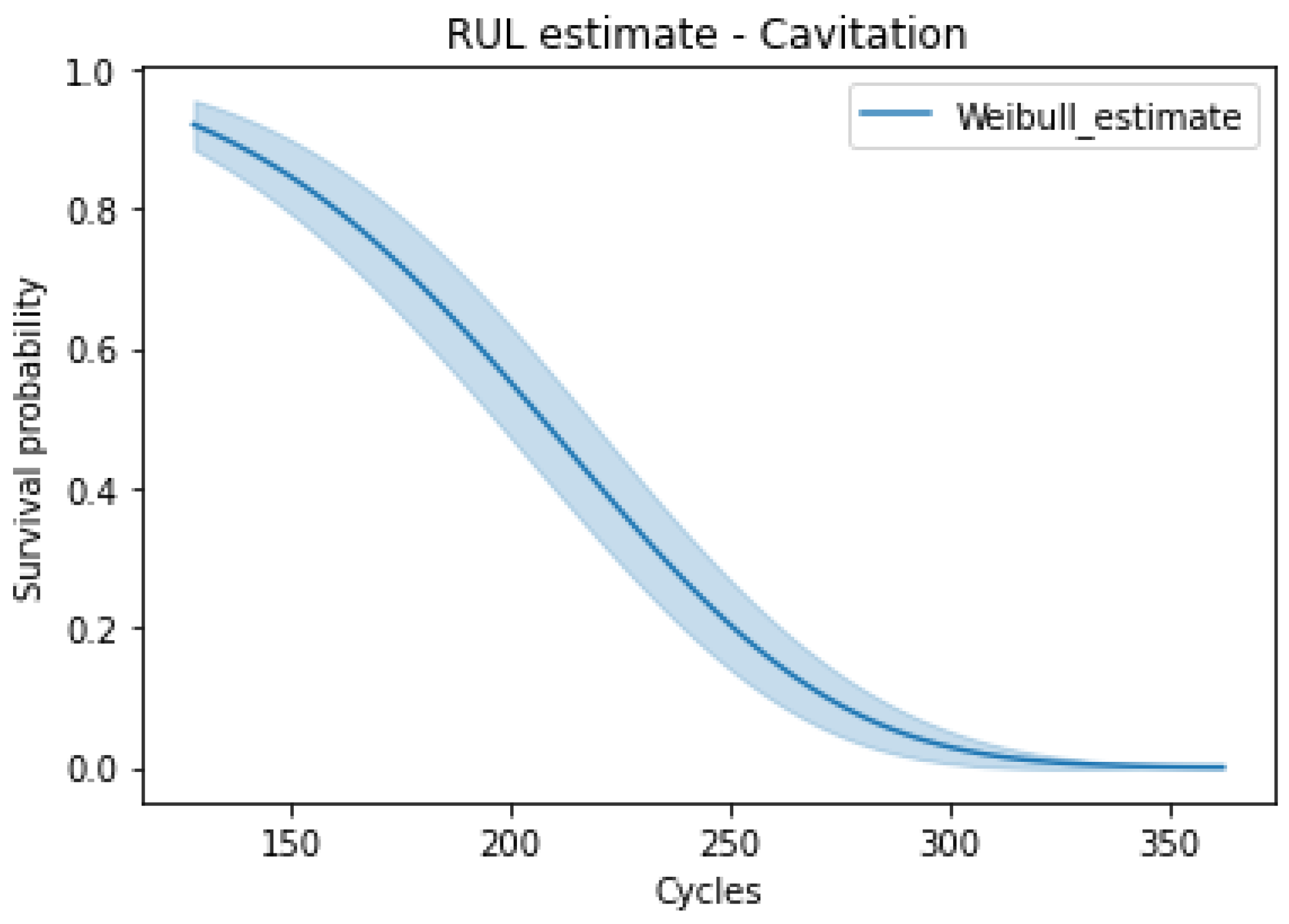
From the Kaplan–Meier plots (Figure 9 and Figure 10), we can observe that all the pumps run for at least 130 operational cycles, then the likelihood of surviving rapidly declines. The Kaplan–Meier estimator provides an accurate description of the survival function of the pump, but due to its non-parametric nature it is difficult to implement in a comprehensive statistical model. To overcome that limit, a parametric model is derived that provides similar estimates.
In this research, the parametric Weibull model is fit to the lifetime data. The Weibull model is defined as
S ( t ) = exp t λ ρ
where λ and ρ are the scale and shape parameters, respectively.
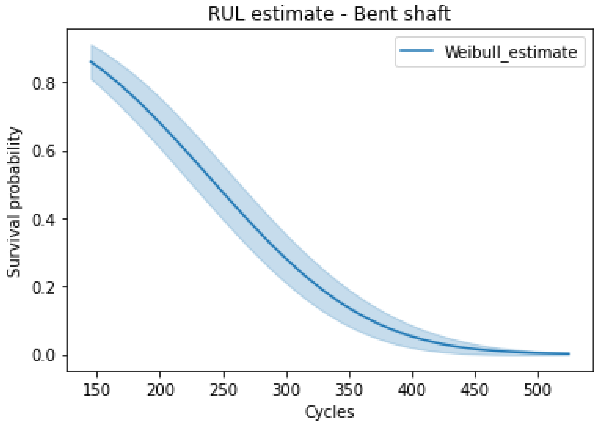
From the Weibull plots (Figure 11 and Figure 12), we observe that the survival function of a pump experiencing cavitation is different than of a bent shaft. This is because each fault affects the pump and its impeller in different ways. Cavitation is much more violent therefore it degrades the impeller quicker that a bent shaft. Thus, the RUL estimate of an impeller due to each fault is also different. Based on this analysis, the survival models are added into the Bayesian network.
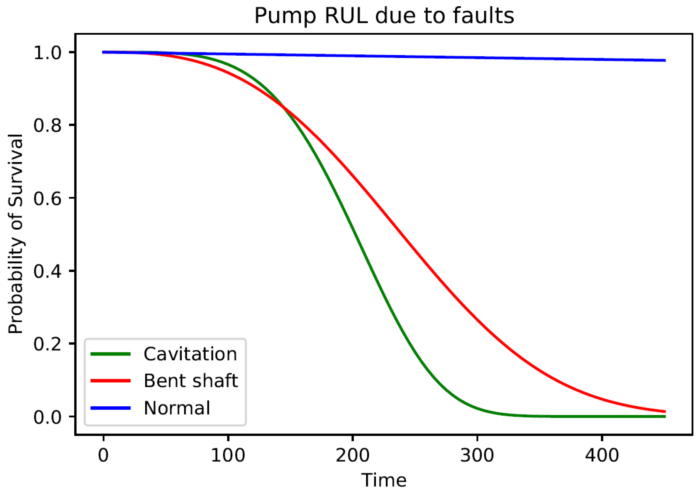
Adding the survival functions for normal and abnormal operation into the Bayesian network provides us with a holistic view of the pump RUL. Figure 13 shows the trajectory of the pump RUL based on a 100% likelihood estimation of the operation mode; i.e., if the Bayesian network estimates that the given vibration measurements are 100% due to cavitation, the pump RUL will follow the green trajectory. Similarly, if the network estimates that the given evidence is 100% due to a bent shaft or normal operation, the pump RUL will follow the appropriate trajectory.
However, a 100% estimate of the state of the pump is usually not likely. This is because of sensor noise as well as the some overlap between the vibration feature values for each operating mode. Therefore, once we provide the network with vibration evidence, it provides a probabilistic estimate of the current state of the machine. Thus, the true RUL lies somewhere between the values shown in Figure 13. This process is further explained in a case study.

4. Case Study

The completed condition monitoring Bayesian network is validated through a case study. To begin testing, additional data sets are created for cavitation. This testing data is then used to diagnose faults and forecast machine health.
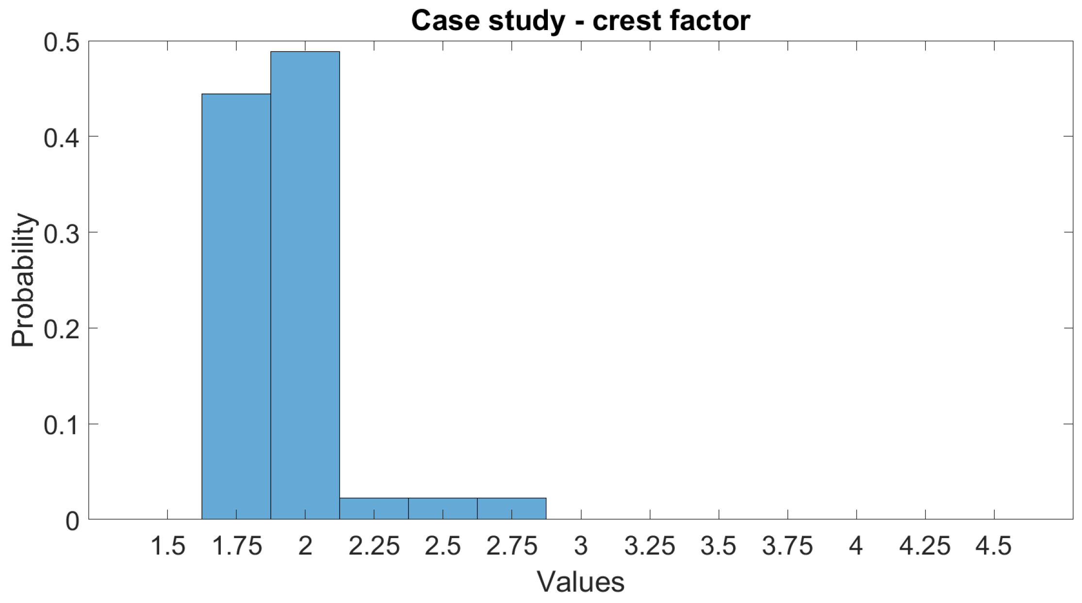
The cavitation testing data consists of vibration information about the high amplitude and frequency disturbances experienced by the impeller. This frequency data is then converted into vibration features so they can be added into the Bayesian network as evidence. However, these vibration features are not constant throughout the collected data as shown in Figure 5, Figure 6 and Figure 7. Furthermore, there is some overlap between the feature values for cavitation, bent shaft, and normal operation. Thus, it is necessary to convert the feature values into a measurement distribution before we can perform the condition monitoring analysis. The overlap in feature values also implies that we cannot estimate the current mode of operation with a 100% certainty.
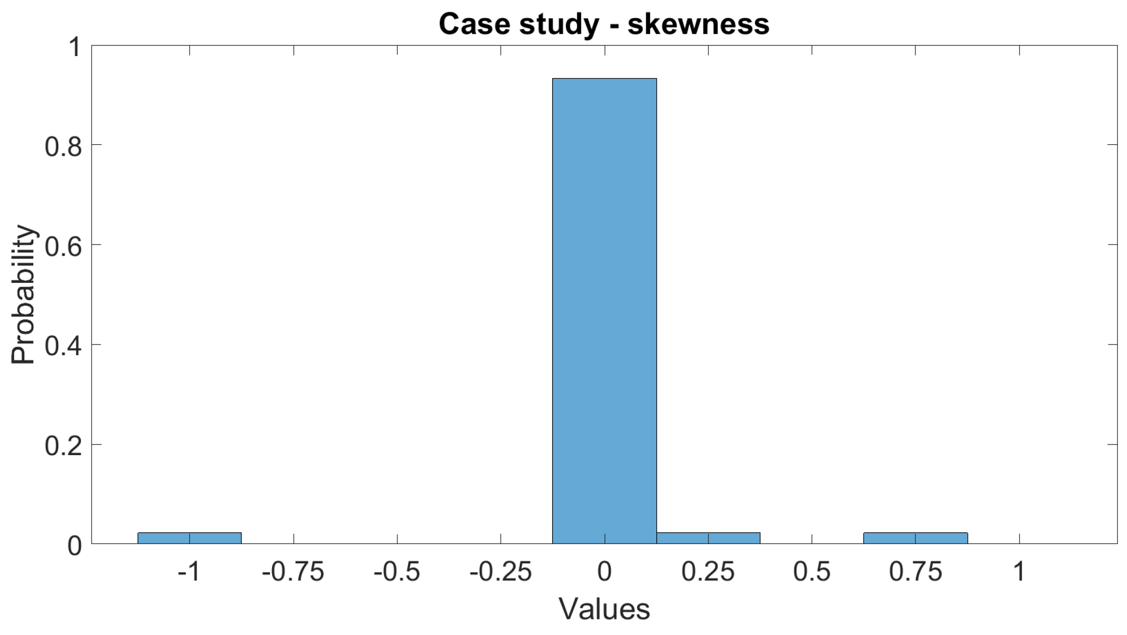
Once these features are translated into a measurement distribution (Figure 14, Figure 15 and Figure 16), they are entered directly into the Bayesian network using SMILE. After we provide evidence, the Bayesian network infers that there is a 95.8% likelihood of cavitation. This is the expected probabilistic result based on the testing data.
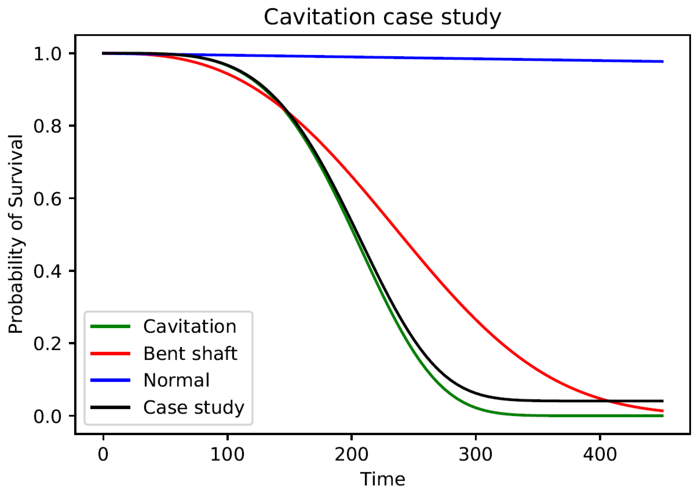
The computation of the pump RUL similarly involves probabilistic estimation. As shown in Figure 13, if the pump is 100% experiencing cavitation, it will follow the green curve. However, since the Bayesian network estimates that the likelihood of cavitation is 95.8%, the estimated survival plot deviates from the green curve, as shown in Figure 17.

5. Results

The case study shows the conditional dependency between the health forecast and the current state of the pump. A set of noisy vibration measurements is provided as evidence to the Bayesian network. The network estimates that there is a 95.8% likelihood for the pump to be experiencing cavitation. Then, the network computes the RUL of the pump based on the survival functions that were developed previously. Given its current state, the pump has a 4% likelihood of survival past 450 operational cycles due to a 95.8% likelihood of cavitation.

6. Discussion

The case study validates the effectiveness of the Bayesian network in inferring the condition of hidden states. Hidden states are processes that are impossible to directly observe. In our condition monitoring system, the occurrence of faults is a hidden state. Using Bayesian networks, we are able to use sensor data and operation information to diagnose and infer the state of the pump.
Using Bayesian networks, we were able to integrate survival models for normal and abnormal operation to predict the RUL of the pump. This integration allowed the health forecast to change conditionally with the state of the pump, thus increasing the estimation accuracy.
This research can be incorporated into a larger asset management framework for industrial machines. Once we know when a machine is expected to fail, we can coordinate with supply chain logistics and business objectives to provide the optimal decision that results in the highest value gained. This would allow us to optimize maintenance resources and reduce operating costs.

7. Conclusions

In this research, we created a condition monitoring framework using Bayesian networks that can estimate and forecast the state of a pump. By doing so, we developed a framework for predictive maintenance using conditional probabilities, sensor data, and operational information. This framework could be deployed to industrial plants where it would be integrated with a probabilistic decision-making system [29].
We determined that a hybrid approach can be used to provide accurate machine health assessments. Incorporating domain expertise to develop models can significantly decrease the amount of data required, as well as improve the transparency of the model. Domain expertise also allows the addition of conditional dependencies, which can be leveraged to infer hidden information.

8. Materials and Methods

The details for this research have been described in Section 3: Procedure.

Author Contributions

Conceptualization, A.K. and D.G.C.; methodology, A.K.; software, A.K.; validation, A.K.; formal analysis, A.K.; investigation, A.K.; resources, A.K. and D.G.C.; data curation, A.K.; writing—original draft preparation, A.K.; writing—review and editing, A.K. and D.G.C.; visualization, A.K.; supervision, D.G.C.; project administration, D.G.C.; funding acquisition, D.G.C. All authors have read and agreed to the published version of the manuscript.

Funding

This research was funded by U.S. Department of Energy, Office of Nuclear Energy’s Nuclear Energy University Program DE-NE0008909 under the Nuclear Energy Enabling Technologies Advanced Sensors and Instrumentation Program.

Institutional Review Board Statement

Not applicable.

Informed Consent Statement

Not applicable.

Data Availability Statement

The data presented in this study are available on request from the corresponding author. The data are not publicly available due to privacy concerns.

Conflicts of Interest

The authors declare no conflict of interest.

Abbreviations

The following abbreviations are used in this manuscript:
NPPNuclear Power Plant
O&MOperations and Maintenance
RULRemaining Useful Life
LSTMLong Short-Term Memory
GPRGaussian Process Regression
CPTConditional Probability Table
GeNIeGraphical Network Interface
SMILEStructural Modeling, Inference, and Learning Engine
EMExpectation Maximization

References

  1. Why Nuclear Outages Are Actually a Good Things|Nuclear Information Center. Available online: https://nuclear.duke-energy.com/2018/03/13/why-nuclear-outages-are-actually-a-good-thing (accessed on 1 December 2022).
  2. Economics of Nuclear Power|World Nuclear Association. Available online: https://www.world-nuclear.org/information-library/economic-aspects/economics-of-nuclear-power.aspx (accessed on 15 November 2022).
  3. Liu, K.; Shang, Y.; Ouyang, Q.; Widanage, W.D. A Data-Driven Approach With Uncertainty Quantification for Predicting Future Capacities and Remaining Useful Life of Lithium-ion Battery. IEEE Trans. Ind. Electron. 2021, 68, 3170–3180. [Google Scholar] [CrossRef]
  4. Chen, Y.; Peng, G.; Zhu, Z.; Li, S. A novel deep learning method based on attention mechanism for bearing remaining useful life prediction. Appl. Soft Comput. 2020, 86, 105919. [Google Scholar] [CrossRef]
  5. Wang, B.; Lei, Y.; Yan, T.; Li, N.; Guo, L. Recurrent convolutional neural network: A new framework for remaining useful life prediction of machinery. Neurocomputing 2020, 379, 117–129. [Google Scholar] [CrossRef]
  6. Wang, W.; Lei, Y.; Yan, T.; Li, N.; Nandi, A. Residual convolution long short-term memory network for machines remaining useful life prediction and uncertainty quantification. J. Dyn. Monit. Diagn. 2021, 1, 2–8. [Google Scholar] [CrossRef]
  7. Zhang, Y.; Xin, Y.; Liu, Z.W.; Chi, M.; Ma, G. Health status assessment and remaining useful life prediction of aero-engines based on BiGRU and MMoE. Reliab. Eng. Syst. Saf. 2022, 220, 108263. [Google Scholar] [CrossRef]
  8. Dong, S.; Wang, P.; Abbas, K. A survey on deep learning and its applications. Comput. Sci. Rev. 2021, 40, 100379. [Google Scholar] [CrossRef]
  9. Li, S.; Fang, H.; Shi, B. Remaining useful life estimation of Lithium-ion battery based on interacting multiple model particle filter and support vector regression. Reliab. Eng. Syst. Saf. 2021, 210, 107542. [Google Scholar] [CrossRef]
  10. N, B.; Chowdhury, R. Remaining useful life (RUL) estimation of lead acid battery using Bayesian approach. J. Electr. Eng. Autom. 2020, 2, 25–34. [Google Scholar]
  11. Benker, M.; Furtner, L.; Semm, T.; Zaeh, M.F. Utilizing uncertainty information in remaining useful life estimation via Bayesian neural networks and Hamiltonian Monte Carlo. J. Manuf. Syst. 2021, 61, 799–807. [Google Scholar] [CrossRef]
  12. Chen, C.; Shi, J.; Lu, N.; Zhu, Z.H.; Jiang, B. Data-driven predictive maintenance strategy considering the uncertainty in remaining useful life prediction. Neurocomputing 2022, 494, 79–88. [Google Scholar] [CrossRef]
  13. Kapuria, A.; Spangler, R.M.; Lois, R.S.; Cole, D.G. Root cause analysis for condition monitoring using Bayesian networks. In Proceedings of the 2022 ANS Annual Meeting, Anaheim, CA, USA, 12 June 2022. [Google Scholar]
  14. Darwiche, A. Modeling and Reasoning with Bayesian Networks; Cambridge University Press: Cambridge, UK, 2009. [Google Scholar]
  15. Advantages of Pressurized Water Reactors|Stanford University. Available online: http://large.stanford.edu/courses/2017/ph241/shaw-s1/ (accessed on 1 May 2022).
  16. Power Reactors|NRC. Available online: https://www.nrc.gov/reactors/power.html/ (accessed on 20 January 2022).
  17. Badr, H.; Ahmend, W. Pumping Machinery Theory and Practice; John Wiley & Sons, Ltd.: Hoboken, NJ, USA, 2014. [Google Scholar]
  18. Brennen, C. Hydrodynamics of Pumps; Cambridge University Press: Cambridge, UK, 2012. [Google Scholar]
  19. Al-Obaidi, A.R. Investigation of effect of pump rotational speed on performance and detection of cavitation within a centrifugal pump using vibration analysis. Heliyon 2019, 5, e01910. [Google Scholar] [CrossRef] [PubMed]
  20. Al-Obaidi, A.R. Detection of cavitation phenomenon within a centrifgual pump based on vibration analysis technique in both time and frequency domains. Exp. Tech. 2020, 44, 329–347. [Google Scholar] [CrossRef]
  21. Reges, G.; Ribeiro, M.; Silva, T.; Abreu, O.; Reis, R.; Schnitman, L. Electric submersible pupm vibration analysis under several operational conditions for vibration fault differential diagnosis. Ocean. Eng. 2021, 219, 108249. [Google Scholar] [CrossRef]
  22. Casoli, P.; Pastori, M.; Scolari, F.; Rundo, M. A vibration signal-based method for fault identification and classification in hydraulic axial piston pumps. Energies 2019, 12, 953. [Google Scholar] [CrossRef]
  23. Zhu, Y.; Li, G.; Wang, R.; Tang, S.; Su, H.; Cao, K. Intelligent fault diagnosis of hydraulic pston pump based on wavelet analysis and improved AlexNet. Sensors 2021, 21, 549. [Google Scholar] [CrossRef] [PubMed]
  24. Vashishtha, G.; Kumar, R. Centrifugal pump impeller defect identification by the improved adaptive variational mode decomposition through vibration signals. Eng. Res. Express 2021, 3, 035041. [Google Scholar] [CrossRef]
  25. Damiano, B.; Blakeman, E.; Phillips, L. Detection and Location of Mechanical System Degradation by Using Detector Signal Noise Data; Technical Report; Oak Ridge National Lab.: Oak Ridge, TN, USA, 1994. [Google Scholar]
  26. BayesFusion, LLC. GeNIe Modeler, SMILE Engine. Academic Version 2.4.4601.0. Available online: http://www.bayesfusion.com/ (accessed on 29 April 2021).
  27. Sammaknejad, N.; Zhao, Y.; Huang, B. A review of the expectation maximization algorithm in data-driven process identification. J. Process. Control. 2019, 73, 123–136. [Google Scholar] [CrossRef]
  28. Davidson-Pilon, C. lifelines: Survival analysis in Python. J. Open Source Softw. 2019, 4, 1317. [Google Scholar] [CrossRef]
  29. Spangler, R.M.; Maccarone, L.T.; Cole, D.G. Modeling operations and maintenance planning decisions under uncertainty using Bayesian networks. In Proceedings of the 2020 ANS Virtual Winter Meeting, Virtual, 19 November 2020. [Google Scholar]
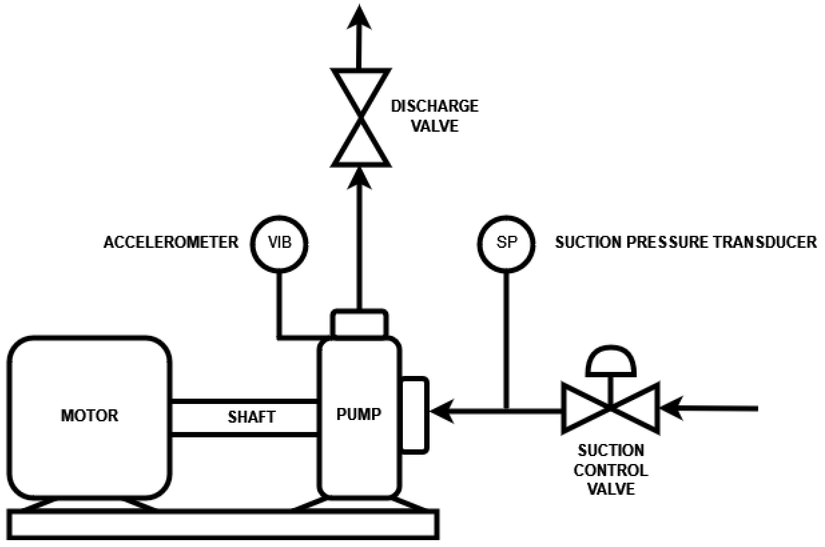
Figure 1. The analyzed pumping system includes a suction valve that controls the flow of water into the pump.
Energies 16 03707 g001
Figure 2. The vibration signal of the pump running during normal operation shows peaks at the vane pass and motor RPM. The motor is running at 3600 RPM (60 Hz). This is evident by the sharp peak at 60 Hz in the figure. The impeller has 6 blades, therefore the vane pass frequency is 6x RPM (360 Hz).
Energies 16 03707 g002
Figure 3. The vibration signal of a cavitating pump shows random high frequency excitation. Along with the vane pass at 360 Hz and RPM at 60 Hz, a cavitating pump also shows a band of high amplitude disturbance between 4 KHz and 20 KHz.
Energies 16 03707 g003
Figure 4. The vibration signal of the pump running running with a bent shaft shows a high amplitude spike at 2 × motor RPM. This peak is indicative of a bent shaft. The other prominent peaks are the vane pass at 360 Hz and RPM at 60 Hz.
Energies 16 03707 g004
Figure 5. The crest factor values of the signal are distinct for cavitation. The y-axis is the normalized crest factor values. The x-axis is the number of samples extracted from vibration data. Each sample contains 10,000 data points consisting of vibration measurements from the pump casing.
Energies 16 03707 g005
Figure 6. The skewness values of the signal are distinct for a bent shaft. The y-axis is the normalized skewness values. The x-axis is the number of samples extracted from vibration data. Each sample contains 10,000 data points consisting of vibration measurements from the pump casing.
Energies 16 03707 g006
Figure 7. The kurtosis values of the signal are distinct for each of the three modes of operation. The y-axis is the normalized kurtosis values. The x-axis is the number of samples extracted from vibration data. Each sample contains 10,000 data points consisting of vibration measurements from the pump casing.
Energies 16 03707 g007
Figure 8. In the Bayesian network, the state of the pump affects the observed values of the vibration features as well as the RUL.
Energies 16 03707 g008
Figure 9. From the Kaplan–Meier plot, we determine that the median life of cavitating pumps is 200 operational cycles.
Energies 16 03707 g009
Figure 10. From the Kaplan–Meier plot, we determine that half of the pumps fail around 220 operational cycles due to a bent shaft.
Energies 16 03707 g010
Figure 11. The resulting λ and ρ values for the cavitation Weibull model are 225.03 and 4.41, respectively.
Energies 16 03707 g011
Figure 12. The resulting λ and ρ values for the bent shaft Weibull model are 276.82 and 2.93, respectively.
Energies 16 03707 g012
Figure 13. The curves in this plot show the RUL forecast for a pump, if the Bayesian network estimates a 100% likelihood for each mode of operation.
Energies 16 03707 g013
Figure 14. The crest factor validation data is converted into a probability distribution for the case study.
Energies 16 03707 g014
Figure 15. The kurtosis validation data is converted into a probability distribution for the case study.
Energies 16 03707 g015
Figure 16. The skewness validation data is converted into a probability distribution for the case study.
Energies 16 03707 g016
Figure 17. Given the current vibration measurements, the Bayesian network estimates that a fault resembling cavitation is most likely occurring. Thus, the forecasted RUL closely follows the cavitation curve, with some deviations due to the inherent uncertainty of probabilistic estimation.
Energies 16 03707 g017
Table 1. A 2050.68 kW (2750 HP) single stage centrifugal feedwater pump is configured for this research.
DescriptionQuantity
Flow, rated0.38m 3 s 1 (6000 gpm)
Head, rated8.96MPa(1300 psi)
Speed59.33Hz(3560 rpm)
Impeller diameter0.46m(18 in)
Efficiency84.05%
Temperature20.00°C(68 °F)
Material selectedCarbon steel
Power, rated1747.18kW(2343 hp)
Power, maximum2231.14kW(2992 hp)
Motor rating2050.68kW(2750 hp)
Table 2. The occurrence of cavitation is discretized into binary states to create the cavitation node.
CavitationPressure Range
Yes0 to 0.21 MPa (0 to 30 psi)
No0.21 to 9.65 MPa (30 to 1400 psi)
Table 3. The occurrence of a bent shaft is discretized into binary states to create the bent shaft node.
Bent ShaftTemperature Range
No−17.8 to 343.3 °C (0 to 650 °F)
Yes343.3 to 482.2 °C (650 to 900 °F)
Table 4. The vibration features are normalized and then discretized to create their respective nodes.
Skewness RangeKurtosis RangeCrest Factor Range
0.75 to 1.003.25 to 3.504.25 to 4.50
0.50 to 0.753.00 to 3.254.00 to 4.25
0.25 to 0.502.75 to 3.003.75 to 4.00
0.00 to 0.252.50 to 2.753.50 to 3.75
−0.25 to 0.002.25 to 2.503.25 to 3.50
−0.50 to −0.252.00 to 2.253.00 to 3.25
−0.75 to −0.501.75 to 2.002.75 to 3.00
−1.00 to −0.751.50 to 1.752.50 to 2.75
2.25 to 2.50
2.00 to 2.25
1.75 to 2.00
1.50 to 1.75
Disclaimer/Publisher’s Note: The statements, opinions and data contained in all publications are solely those of the individual author(s) and contributor(s) and not of MDPI and/or the editor(s). MDPI and/or the editor(s) disclaim responsibility for any injury to people or property resulting from any ideas, methods, instructions or products referred to in the content.