Power Output Optimisation via Arranging Gas Flow Channels for Low-Temperature Polymer Electrolyte Membrane Fuel Cell (PEMFC) for Hydrogen-Powered Vehicles

Abstract

As we move away from internal combustion engines to tackle climate change, the importance of hydrogen-powered vehicles and polymer electrolyte membrane fuel cell (PEMFC) technology has dramatically increased. In the present study, we aimed to determine the optimal configuration for the power output of a PEMFC system using computational fluid dynamics (CFD) modelling to analyse variations of the primary serpentine design of gas flow channels. This helps improve efficiency and save on valuable materials used, reducing potential carbon emissions from the production of hydrogen vehicles. Different numbers of serpentine gas channels were represented with various spacing between them, within the defined CFD model, to optimise the gas channel geometry. The results show that the optimum configuration was found to have 11 serpentine channels with a spacing of 3.25 mm. In this optimum configuration, the ratio between the channel width, channel spacing, and serpentine channel length was found to be 1:2.6:38 for PEMFCs. Furthermore, the inclusion of fillets to the bends of the serpentine gas channels was found to have a negative effect on the overall power output of the fuel cell. Moreover, the optimisation procedures with respect to the number of gas channels and the spacing revealed an optimal power density exceeding 0.65 W/cm².

1. Introduction

As governments set “net zero” carbon emission targets, hydrogen power and technology are becoming increasingly relevant, competing with other sources of clean and renewable energy, such as solar, wind, and biofuels. Batteries and hydrogen are a significant energy storage technology that have the potential to mitigate and lessen the harm being inflicted on the environment, especially for hydrogen and electric car applications [1]. Hydrogen fuel cell technology was invented in 1932 by Francis Thomas Bacon, but has rarely been commercialised in the motor industry due to the lack of hydrogen fuel stations and infrastructure. However, the future of hydrogen-powered vehicles (HPVs) is looking bright, with governments setting low carbon targets and the banning of sale of internal combustion vehicles in the UK by 2030. Additionally, there will be more renewable electricity sources as we move towards a greener economy. There will be more excess electricity produced during peak output periods, and this excess electricity can be stored as hydrogen through electrolysis, ready to be used in HPVs. With the emphasis moving away from hydrocarbon fuel for vehicles, hydrogen is an attractive alternative fuel source, with much higher energy density than hydrocarbons and faster re-fuelling times than electricity and batteries. However, one of the problems with producing hydrogen-fuelled vehicles is that they do not compare favourably with the power output and acceleration of electric vehicles. CFD analysis of low-temperature PEMFCs used in hydrogen-powered vehicles can be used to optimise the gas channel configuration of the PEMFCs that are stacked within HPVs to increase the power output of the vehicle. Hydrogen fuel cell (HFC) technology is and has been thought to be a viable green low-carbon alternative to the internal combustion engine. HPVs are 64.7% fuel efficient compared to 20.8% for internal combustion engines over one drive cycle [2].

PEMFCs use hydrogen compressed gas and oxygen from the air to generate electricity and water. HFCs have two sides, a hydrogen gas side with the anode and an oxygen side with the cathode. The electricity is generated by the polymer electrolyte membrane (PEM) blocking the movement of electrons from the hydrogen side to the oxygen side, or from one gas diffusion layer electrode to the other. This means that the hydrogen ions can pass through the membrane, leaving the electrons to react with the oxygen from the air. With nowhere else to go, the electrons run up the anode and down the cathode, generating electricity. The oxygen then reacts with the electrons from the cathode and the hydrogen ions, producing water as a waste product. Catalysts like platinum allow hydrogen molecules to be split into protons and electrons on the anode side. Furthermore, on the cathode side, the platinum catalyst enables oxygen reduction by reacting with the protons generated by the anode. These enhanced dynamics decrease the reaction temperature in the PEMFC, to a lower temperature for use in the HPVs below 80 °C [3].

The PEMFC working principle is based on the gas that flows into the cell through gas channels that are connected to bipolar conductive plates or ‘flow plates’ for the flow of electrons. The gasses then diffuse into a layer called the gas diffusion layer (GDL). This is where the hydrogen-oxygen reaction occurs as the gasses react with the catalyst’s assistance. There can be a layer between the catalyst and GDL called the micro porous layer (MPL) used to reduce water content in the reactive area up against the catalyst [4]. Each fuel cell has a certain standard flow channel configuration within HPVs. These fuel cells are stacked in arrays to increase output. Therefore, any optimised design needs to be stackable. They can be stacked in series to increase voltage or in parallel to increase the current, according to the needs of the vehicle. Usually, in HPVs, wired connections are inefficient. Therefore, a bipolar plate connection is generally used [3].

PEMs are known as the ‘heart’ of an HFC and are one of the most critical areas to understand. One of the main causes of failure in an HFC is the degradation of the PEM. These polymers, with ions attached to them, have a negative charge, repel electrons, and attract hydrogen ions [5]. Early PEMs only had a lifetime of 200 h at 60 °C and were made using a sulfonated polystyrene backbone. Currently, the most commonly used PEM is Nafion 120 [5]. A Nafion PEM has a lifespan of 60,000 h, operating at a temperature of 22–82 °C at one atmospheric pressure [5]. The lifetime of a PEM determines the lifetime of a PEMFC and is critically important. Mechanical degradation can occur due to the fragility of the material, especially when using thin membranes. Non-uniform pressure between the membrane electrode assembly and the bipolar plates in the system can accelerate this degradation [5]. Degradation is significantly increased when low humidity, high pressure and temperature are applied simultaneously. Penetration of catalyst particles into the membrane can cause local areas of high stress, resulting in an increase in the acceleration of degradation [5]. Nafion 120 is different from most PEMs, with a higher mechanical stability due to its polytetrafluroethylene backbone [5]. This allows a thinner PEM layer and therefore reduced ohmic internal resistance.

Another way a fuel cell can fail is cell reversal. This occurs when oxygen forms at the anode due to localised water electrolysis. This cell reversal causes the current to flow outside the channels due to the high water content. This can be prevented by adding MPLs into the PEMFC [6]. This layer is situated between the catalyst and the gas diffusion layer (GDL). It uses large pores in its material composition to separate and transport water produced in the hydrogen-oxygen reaction away from the reactive area up against the catalyst, allowing more reactants to collide with the catalyst, thereby increasing power output and efficiency of the PEMFC [4].

Chemical degradation is another area that is a cause of failure of PEMs. During use, there is a small chance that radicals (a particle with one unpaired valence electron) can be formed and these radicals attack carbon-hydrogen bonds, causing degradation of the PEM [7]. A platinum catalyst was found to negate the production of most of these radicals due to the occurrence of other catalytic reactions that can occur in its presence [5].

Humidity within the GDL and MPL impacts the power output of an HFC. One study used a CFD model of one gas channel within a PEMFC to measure how humidity affects power output [8]. It was discovered that the cell’s performance at low humidities was influenced by the ohmic polarisation within the cell. Excessive humidity on the cathode side causes the catalyst to flood with water, resulting in a loss of performance. The water forms between the GDL and the catalyst interface [9]. Higher bipolar plate temperatures can be used to prevent this, as less water is able to condense. Alternatively, a dehumidifier can be used before the inlet [8]. However, this is not possible for low temperature PEMFCs used in HPVs, so other solutions are needed. An MPL layer helps prevent flooding by managing the water content in the GDL and reducing the effect of water flooding on the fuel cell’s performance by allowing reactant gasses to reach the catalyst layer [6]. Another way of increasing the cell’s performance by removing water content is by inserting porous sponges into the serpentine flow field [9].

An area of contention In PEMFC gas channel configuration research is co-current flow vs. counter-flow between the anode and cathode sides of the fuel cell. One model, using co-current flow, found that serpentine channels have better performance than parallel flow channels [10]. Multiple serpentine flow models either use co-current flow with gas channels directly above each other or counter-flow with the gas channels running between each other from the cathode to anode sides [11]. Most models seem to do one or the other, and both models appear to be almost as effective as each other [12]. When channels are lined directly above each other, co-current flow has been found to have the highest power output [13]. There has been much discussion over which model is best. A recent study by Yuan et al. compared these models using current density data and found that the counter-flow model was better for creating the highest power output [12]. However, this study employed more hydrogen, so it can be argued that the co-current model is more efficient, as hydrogen fuel lasts longer when the cell is running. Due to the higher power output in the counter-flow model, the authors only consider this model in this research. Based on the earlier study, HPVs and PEMFCs are more relevant in this field, as the world will move to more carbon-neutral technology and increase the engine’s power and performance. This study implemented a CFD model of low-temperature PEMFC, using data and equations from the Ansys PEMFC module manual [14] to create an initial model of a PEMFC. The data and the parameters—including the boundary conditions from the literature—were used to validate the model, together with a set of potential differences and power density comparison. Moreover, this study illustrates the optimum voltage for the highest power output and uses CFD software to optimise the number of air and hydrogen serpentine gas channels within a single PEMFC. In addition, this research aimed to utilise a new model to design different numbers of channels to find the configuration with the maximum power density output across the PEM of the HFC. However, the geometry of the highest power density number of channels will be further optimised by comparing standard 90-degree bend gas channel bends and filleted curved gas channel bends of different radii to find the highest power density and to find the best gas channel configuration overall.

The novelty and research work in this study includes:

• The development of a new CFD model for low temperature PEMFCs—using data and equations from the ANSYS PEMFC module—validated with a set of potential difference and power density plots against current density, to compare with existing literature.
• CFD modelling is used to optimise the number of air and hydrogen serpentine gas channels within a single PEMFC, where we use the new model to design different numbers of channels to find the maximum power density output across the PEM of the HFC.
• We use potential difference and power density to work out and illustrate the optimum voltage for the highest power. The PEMFC geometry is optimised by comparing standard 90-degree bend gas channel bends with filleted curved gas channel bends of different radii to find the highest power density and the best overall gas channel configuration.

2. Theory and Methodology

A similar experiment to this research has been conducted by Ferng et al. [14]. However, the previous investigation solely focused on the most common serpentine bend channel shape and parallel channel shape. An area of contention at that time was whether a serpentine channel shape was better than a parallel flow shape for the reactant gas flow channels. The purpose of this research is to address this question. For the validation, the d’Adamo et al. modelling case study will be used with a 25 cm² active area of the PEMFC and a set 0.7 V potential at relative humidity inlets of 100% with an operating temperature of 300.15 K [15]. In this study, a ‘sweep’ function was used on the membrane electrode assembly to increase mesh density, and therefore the accuracy of the results. The higher the mesh density around boundaries, the more accurate the results relating to the linear flow boundary layer thickness where the wall affects the velocity of the linear flow. The first layer of all inflations should be the same as the thickness of the boundary layer [15]. This meshing method, using sweeps and inflations, can increase the PEMFC model’s accuracy. Furthermore, this study used similar boundary conditions of d’Adamo et al. to compare the PEMFC model [15]. Regarding the boundary conditions, it has been found that it is best to have a constant pressure from the inlet to the outlet in order to achieve the highest electrical power output [13]. This also means that improved gas channel configurations will have a low pressure drop.

Table 1. Channel and Membrane Electrode Assembly Parameters.

Part	Direction	Dimension (mm)
Domain	[X,Y,Z]	[50,50,2.68]
Gas Channels	Section Width	1.25
	Section Height	1.25
	Length of serpentine branches	48
	distance between serpentine branches	1.25
GDL	[X,Y,Z]	[50,50,0.1273]
Membrane	[X,Y,Z]	[50,50,0.0254]

shows all the channel configuration parameters used in the analysis and validation.

2.1. PEMFC CFD Modelling

This research uses Ansys fluent 2021R1 to model PEMFC channel configurations. The models were formulated using the Ansys Fluent PEMFC add-on module manual, listing all of the modelling software’s governing equations [16,17,18,19], including the information on the many processes and energy losses that are less known within HFCs. The main reasons for choosing this software lie in the ability to solve complex fluid flow problems numerically and to simulate coupled models with multiple variables needed for a PEMFC as a laminar flow model [20,21,22,23]. This research is split into three different model sections, including an initial model that set out and ran a simple model to gain insight into polarisation (potential difference) and power density curves for the default parameters embedded in the Ansys fluent module [14]. The next set of models validated a polarisation curve against the literature and their experimental results using the same geometry. Finally, the third set of models used different geometry to optimise the design of the reactant gas channels within that same model.

In the simulation, Navier stokes equations are used to model fluid flow applied across a mesh of cells, in which individual momentum vectors are calculated using numerical methods. These are then used to convert a set of partial differential equations over iterations into solvable equations. The model follows the conservation of mass from the inlet and outlet boundary conditions, and the total energy is used to model static and dynamic temperature throughout the model from the hydrogen-oxygen reaction.

The current flux equation was activated through modelling the PEMFC because of the existence of electrochemistry, and to model the movement of current [14]. Electrochemistry modelling equations can be used to model the flow of current through the materials within the PEMFC by setting a voltage potential at both ends of the PEMFC on the anode and cathode side as fixed boundary conditions; the initial current flux R at the anode and cathode can be found. The calculations are also explained by a current flux boundary condition that is ready to be identified numerically towards the centre of the mesh, and therefore at the PEM. The current flux total can be found across the membrane by an integral method across a plane area at the centre of the PEM, giving the model results [14]. This process is repeated using different gas channel configurations for optimisation. One of the primary energy losses in PEMFCs is the activation loss due to the slowness of the hydrogen-oxygen reaction taking place near the membrane surface [24]. This is usually found by subtracting the potential difference at the membrane from the potential at the flow plate on the anode side [14].

In the post-processing of CFD results, several numerical calculations need to be carried out to gather relevant outcomes, such as polarisation and power density curves. The fundamental equation for calculating electrical power can be stated as follows:

$$P=VI$$

(1)

where P represents the power (W), V is the potential difference (V), and I is the current (A). This equation characterises the fundamental to the measurement of power output of fuel cells from a fixed voltage and a measured current density. Therefore, this equation needs to be modified to suit the current density measurement as follows:

$$P_d=V{I}_d$$

(2)

where $P_d$ is the power density ($\mathrm{W}/{\mathrm{m}}^2$), and $I_d$ represents the current density ($\mathrm{A}/{\mathrm{m}}^2$). The power and current densities are calculated over the active area of the PEMFC. Current density is gathered from the CFD results across the centre plane of the PEM. This is then converted into the power density curve of the PEMFC at different fixed voltages.

2.2. Defining Material Properties

There were two sets of material properties used in the experiment. The first set was the default Ansys values for the material for the initial model, and the validation properties as seen in

Table 2. Properties of Graphite and Nafion.

PEMFC Part	PEM	Flow Plate Electrodes
Material	Nafion	Graphite
Density (kg/m3)	1970	2250
Electrical conductivity (S/cm)	1 × 10−16	125,000
Thermal Conductivity (W/m K)	0.445	20
Specific Heat (J/kg K)	903	707.68

. The default Ansys properties are described in

Table 3. Ansys default material properties.

Material Represented	PEMFC Part	Density (kg/m3)	Specific Heat J/kg·K	Thermal Conductivity W/m·K	Electrical Conductivity (S/m)
graphite	flow plate	2719	871	100	1,000,000
	GDL	2719	871	10	5000
Epoxy	MPL	2719	871	10	5000
Platinum	catalyst	2719	871	10	5000
Nafion 120	PEM	1980	2000	2	1 × 10−16

.

Table 3 shows the material properties that arise automatically when Ansys fluent is released. This was used as the initial models’ materials. Although the GDL layer is assigned material for electrical and thermal conduction purposes, in reality, the layer is just space for the reactant gasses to diffuse into. The material properties for the validation and optimisation models used the properties shown in Table 2 for the flow plate and PEM layers. The other layers were modelled with the same density as the flow plate in Table 2. This was so that the model could be simplified to represent any set of materials for any PEMFC. The thermal conductivity, specific heat, and electrical conductivity were kept the same as the default properties to decrease the chance of error in the model due to the change in properties from the initial model to the validation model. The material properties for the validation model are shown in

Table 4. Validation Model Material Properties [15].

Material Represented	PEMFC Part	Density (kg/m3)	Specific Heat /kg·K	Thermal Conductivity W/m·K	Electrical Conductivity (S/m)
graphite	flow plate	2250	707.68	20	1.25 × 107
	GDL	2250	871	10	5000
Epoxy	MPL	2250	871	10	5000
Platinum	catalyst	2250	871	10	5000
Nafion 120	PEM	1970	903	0.445	1 × 10−16

.

2.3. Biconjugate Gradient Stabilisation Method (BCGSTAB)

The BCGSTAB method is used to solve non-symmetrical linear systems while helping avoid irregular convergence patterns. This helps stabilise variables that may have irregular fluctuations in value while the model runs. In the context of an HPV, these variables would be controlled and regulated by subsystems within the HPV. When the variable starts fluctuating, usually at the beginning of a set of iterations, the residual of the variable will return to a stable set of values and begin to converge, thanks to the BCGSTAB method. During the running of the models, the species molar counts and the electric and protonic potential variables use BCGSTAB. The species molar counts used the BCGSTAB method because the reactant content in the early iterations of the model can drop very suddenly due to the reaction taking place, and the water content can increase significantly as a waste product. The electric and protonic potential would likely be controlled by a set of diodes to prevent current in the opposite direction and circuit breakers. The BCGSTAB method assisted with getting convergence in the model and helped prevent floating point exemption errors. These errors are caused by a large gradient in the residuals of the model, meaning that the governing Navier stokes equations divide by zero resulting in an invalid result.

2.4. F-Cycle Method and Coupled 2nd Order Modelling

The F-cycle multigrid method was used for all calculated variables within the models. This technique is used to speed up the solution and convergence of an iterative model. It reduces the number of iterations needed for convergence, utilising a set of simultaneous correction equations. This method adds neighbouring discretised equation coefficients and generates these correction equations. These coefficient additions allow the correction equations to be solved using fewer iterations. The F-cycle has a faster solution time than a V-cycle due to more coefficients making up correction equations. This saves computational power and time, and because of these advantages, the F-cycle was used in the initial and validation models.

The model used a coupled solver that solves for continuity, momentum, energy, and species simultaneously, due to it saving computational power compared to other methods. The models use a second-order scheme which is second-order accurate in terms of the Taylor series as a model. All models had a courant number of 200, which is the speed of sound multiplied by the ratio of the time step length to the cell length. Throughout the F-cycle modelling process, there are several errors that can occur, including data errors, syntax errors, logic errors, and parameter errors. These can be avoided by double checking input parameters before running the model, thoroughly assessing the CFD, F-cycle, and BCGSTAB code before use, and ensuring that the digital inputs are within their acceptable range [25].

All additional parameters used in the simulation which support the verification based on the boundary conditions are listed in

Table 5. Further Boundary conditions for the Ansys fluent PEMFC add-on module.

Boundary Condition Input	Value
W-diff Model	Wu
Liquid vapour source relaxation factor	0.2
Devised vapour/liquid relaxation factor	0.2
Osmotic drag relaxation factor	1
Gas diffusion layer liquid removal	0.5

and

Table 6. Anode and Cathode Inlet and Outlet Boundary Conditions.

Region	Surface	Property	Value
Anode	Inlet	Mole Fraction H2	0.9764
		Mass Flow Rate (kg/s)	3.93 × 10−7
		Pressure (bar)	1.5
		Temperature (K)	300.15
		Mole Fraction H2O	0.0236
	Outlet	Mole fraction H2, H2O	0.9764, 0.0236
		Pressure (bar)	1.5
		Temperature (K)	300.15
Cathode	Inlet	Mole Fraction O2	0.2075
		Mass Flow Rate (kg/s)	2.07 × 10−5
		Pressure (bar)	2
		Temperature (K)	300.15
		Mole Fraction H2O	0.0119
	Outlet	Mole fraction O2, H2O	0.2075, 0.0119
		Pressure (bar)	2
		Temperature (K)	300.15

.

3. Model Descriptions

3.1. Physical Model

First, a geometry was needed to carry out the modelling and optimisation. This was found by using the example model case study as a guide to create a similar geometry to validate the Ansys model [13]. One difference intended between this model and the PEMFC model is the inclusion of an MPL layer. As noted above, this is an extra layer in the fuel cell between the Catalyst and GDL layers that removes water content. This means that the liquid phase of the model can be removed, saving computing power, and this causes better convergence in models. The model used the 25 cm² active area from the case study model, as shown in Figure 1. To simplify, the channels were assumed to have 90-degree corners, to get a standardised set of results that could be used for any fuel cell. The model used the same materials as in the literature.

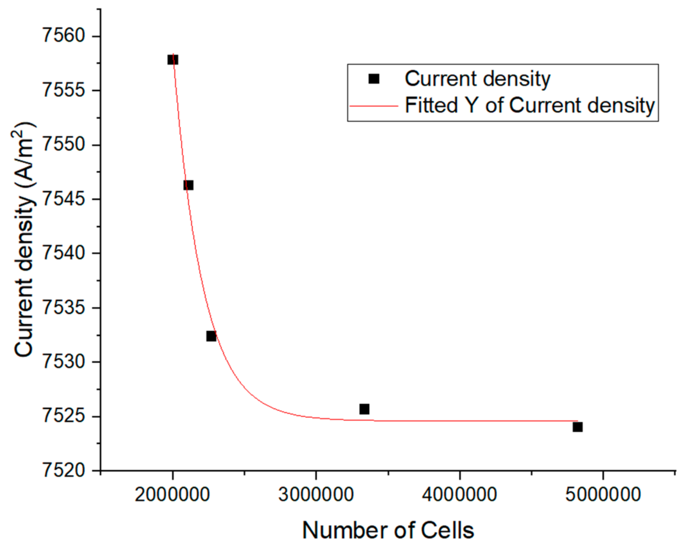
3.2. Meshing and Mesh Dependency Analysis

For the PEM meshing, a sweep method was used with one division to save computational power, because it is a very thin layer. The catalyst and MPL layers had three division sweep methods because that is where most of the reaction is taking place, and increasing the mesh density captures the change in temperature and species gradients more accurately. The GDL would also be ideal for sweeping, but due to the irregular surface of the gas channels, it is not possible to compute. Therefore, the GDL was computed with trapezoidal cells, ensuring that they are pyramidal cells close to the sweep method of the MPL layer, to increase accuracy. The gas channels have an inflation layer around them to increase the accuracy of the flow results around the walls of the channels. This inflation was three layers thick and had a growth ratio of 1.2. The flow plates were left with a standard trapezoidal mesh with a standard cell size from meshing software (3.55 mm). This was to save on computational power and had the benefit of the mesh being adaptable for any configuration of gas channels.

To find the best cell size for the MEA, GDL, and gas channels, the initial Model was run with different cell sizes for each to find the set that saved the most computational power while getting the most accurate results. To get the pyramidal cells in the GDL layer of the mesh, the cell size needs to be half of the MEA (PEM, MPL, and catalyst layers) cell size. In addition, due to the inflation giving high accuracy in the gas channels to save on computational power, the cell size in the gas channels is set to double that of the MEA. Each cell size set from every layer gave a different number of cells to run in the model. The results of this are shown in

Table 7. Layer cell size to cell number.

Cell Size Flow Channels [mm]	Cell Size GDL [mm]	Cell Size MEA [mm]	Number of Cells
1.5	0.375	0.75	2,000,968
1.25	0.3125	0.625	2,109,151
1	0.25	0.5	2,270,056
0.75	0.1875	0.375	3,333,827
0.6	0.15	0.3	4,820,839
0.625	0.25	0.5	2,403,259

and Figure 2.

Figure 2 below shows how current density across the PEM from the initial model exponentially decays with cell number to an asymptote around 7525 A/m². This is the ideal point to choose, as the cell size of the layers would be at the bottom of the exponential curve, as it flattens out. However, to save computational power and reduce the models’ run-time, 1 mm for flow/gas channels was chosen, with 0.5 mm for the MEA and 0.25 mm for the GDL layers. Figure 3 below shows the final mesh used in the models with the sweep methods and inflations.

3.3. Initial Model Setup and Boundary Conditions

To get the first model setup, named sections for each layer body were created, following the Ansys PEMFC module manual [14]. Similarly, for the cathode’s and anode’s inlets and outlets, it was important to ensure that the inlets of the anode and cathode are above and below each other for counter-flow to occur. Furthermore, to control voltage, named sections on the top and bottom surfaces were created for the cathode and anode terminals. Within the PEMFC add-on module, each named section body layer needed to be added to their respective chosen layer within the software for the anode and cathode (flow/gas channels, flow plates, GDLs, MPLs, catalyst layers, and the PEM). This model was run for over 200 iterations.

First, a contact resistivity was added to model an imperfect contact between flow plates and the GDL layer of the PEMFC. This contact resistivity was $1\times {10}^{-6}{ \mathsf{\Omega }\mathrm{m}}^2$ as a general value used [14]. The simulation temperature was set to 333.15 K as an operating temperature.

The anode and cathode inlets were mass flow inlets with flow rates of $1\times {10}^{-7} \mathrm{kg}/\mathrm{s}$ and $1.4\times {10}^{-6} \mathrm{kg}/\mathrm{s}$, or inlet velocities of 0.064 m/s and 0.896 m/s, respectively. The cathode needed a higher mass flow rate to account for the lower reactant content, as oxygen only makes up roughly 20% of the air [14]. Therefore, for this model, the species content was set up as mass fractions, the same for the inlet and outlet. For the cathode, oxygen was a mass fraction of 0.2 and a water content of 0.17. Additionally, for the anode, the hydrogen mass fraction was 0.5, and 0.5 for water content. To best model, simplify, and optimise the gas channel configuration, a constant liner flow was used with constant pressure and species content for the anode and cathode sides of the PEMFC model. The Reynolds number for the anode and cathode were 11.3 and 91.8, respectively. For the initial model, one atmospheric pressure was used as the operating pressure. The anode terminal was set at 0 V potential difference, and the cathode terminal was set to different voltages for the polarisation curve. This was from 0.8 V to 0.2 V, repeating the model each time. The initial model material properties were implemented in this model to get a set of polarisation and power density curves.

3.4. Validation Model Setup and Boundary Conditions

The contact resistivity from the validation model was kept the same as in the initial model. The boundary conditions were taken from the literature [15]. All other boundary conditions were kept the same as in the initial model except for the values shown in

Table 8. Validation model boundary conditions.

Boundary Condition	Set Value
Temperature (K)	300.15
Anode Mole Fraction H2	0.9764
Cathode Mole Fraction O2	0.2075
Anode Mole Fraction H2O	0.0236
Cathode Mole Fraction H2O	0.0119
Pressure (Pa)	175,000

.

The case study model runs two different pressures for the anode and cathode. This method is not possible using Ansys fluent because the solid-fluid modelling of the PEMFC MEA causes the model to fail with floating point exemption errors due to the pressure gradient in the system. Therefore, the pressure chosen for the validation model of 175,000 Pa was between the two anode and cathode pressures from the literature [15]. The mass flow rates of the inlets were kept the same as the initial model, and for the same reason, they were set up due to the different pressures. This may lead to different results from the literature. The temperature chosen was the same as the literature’s model [15]. The validation model gives a set of polarization and power density curves relating to the literature. This will provide the fuel cell’s optimum power output, which can then be used in geometry variation and optimisation models. Additionally, a contour of the current density was taken across the PEM to show where the most electrical power is being generated in the cell through the hydrogen-oxygen reaction. This model was run for over 500 iterations.

3.5. Geometry Variation

During the research, many sets of similar geometry were used for different serpentine flow channels. Figure 1 shows the initial 19-channel configuration. The outer two channels with the inlets and outlets were fixed. To optimise the PEMFC serpentine gas channel configuration, the number of gas channels for both the anode and cathode was reduced by two each time from nineteen down to three channels. The spacing between the channels was found using Equation (3), with 46.35 mm being the distance between the two outer channels:

$$Channel Spacing\left(\mathrm{m}\mathrm{m}\right)=\frac{\left(46.35-1.25\times N\right)}{\left(N-1\right)}$$

(3)

where N represents the number of serpentine gas channels. The spacing was implemented so the channels were evenly spaced as if the set of gas channels were continuous and could be implemented into a stack of cells. These new PEMFCs can be modelled to find the power density of the new configurations. Therefore, it was possible to find the best power output configuration, which can be used to test different fillet radii. Additionally, a contour of the current density was taken across the PEM, to show where in the cell the most electrical power was being generated through the hydrogen-oxygen reaction for the optimum number of channels.

3.6. Fillet Radii Testing

The serpentine channels for each configuration have used 90-degree squared-off bends. This configuration can now be compared to filleted channels (with rounded bends) by testing whether filleting these bends can increase the power output of the PEMFC. The original 19-channel configuration and the best geometry from the geometry variation were tested. Bends in the serpentine channels were modelled with different radii for comparison purposes. These were then put through the validation model at the optimum power output voltage to find the highest power outputting fillet radius. This was performed from a fillet radius of 0 mm to 1.625 mm for the optimum number of channels. Furthermore, for the original 19-channel configuration, filleted and 90-degree corners were tested from a radius of 0.625 mm. These results made it possible to find the optimal geometry for a PEMFC.

4. Results and Discussion

This CFD study compared the modelled results to experimental results and discovered an underestimation of the current density of the membrane at lower fixed voltages [15]. The authors thought that this was due to the uncertainty in material characterisation. The model and results were plotted on a polarisation/power density curve shown in Figure 4.

Figure 4 will help compare the validation model of this research against the case study’s experimental and model results. The validation model is intended to validate the CFD model by getting similar characteristic results to Figure 4 and getting as close as possible numerical values to this study’s experimental results. The potential difference against current density can be plotted for different fixed voltages, and the power density can be calculated from each current density.

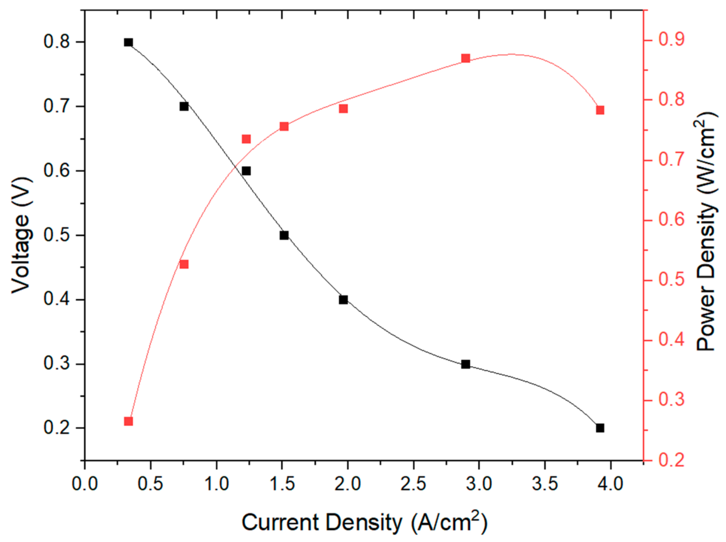
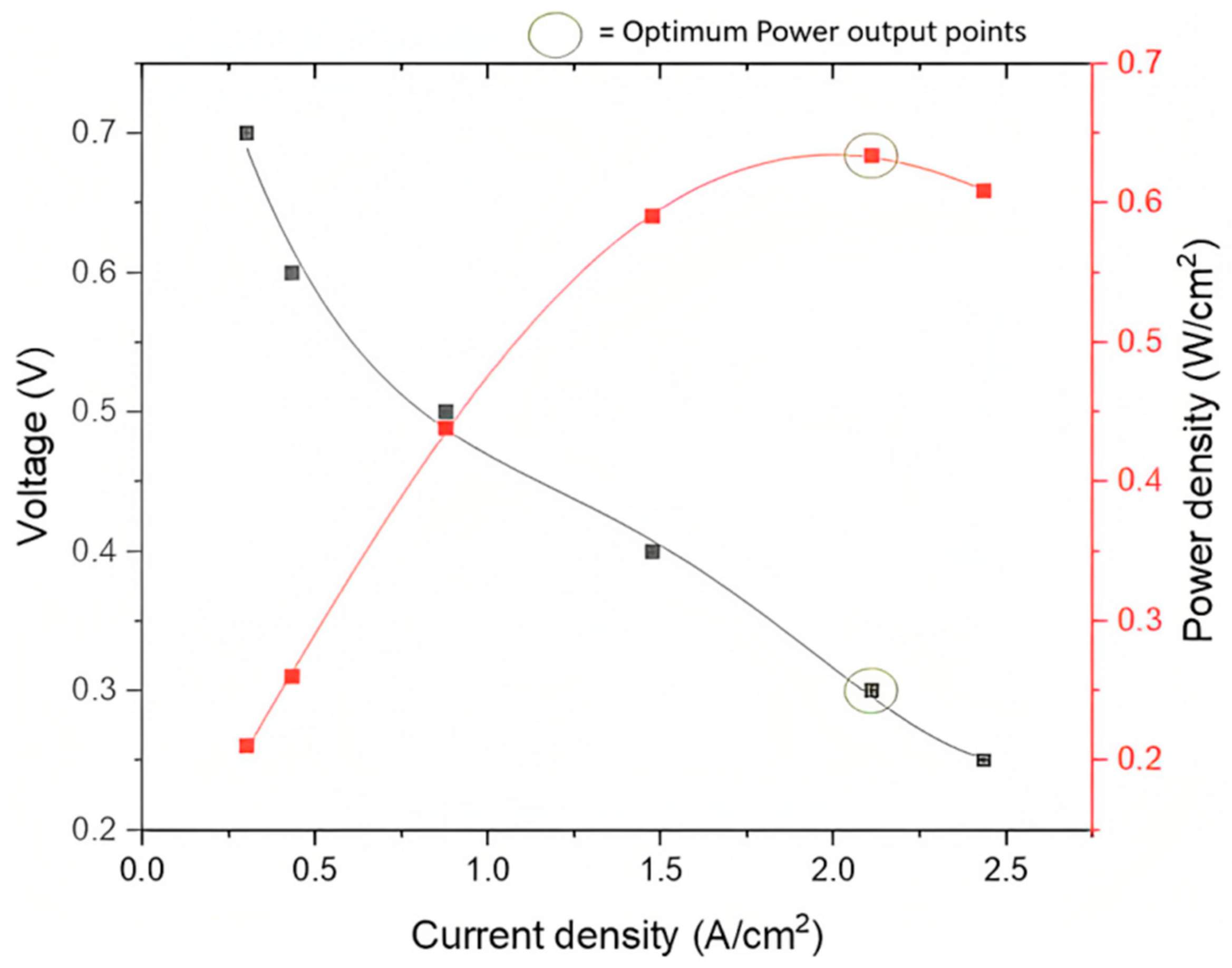
4.1. Initial and Validation Models Polarization and Power Density Graphs

The figures in this section present the data collected from the experimental work. Figure 5 and Figure 6 present how voltage and power density vary with current density for the initial model and validation model, respectively. The behaviour of the validation model results in Figure 5 are very similar to that of the experimental results in the literature shown in Figure 4. The validation model also shows a peak power density output at 0.3 V. Therefore, this is the optimum power output voltage ready to be used as the voltage for the geometry variation. That is 83.3 cm² of active area for every volt of potential difference. For the initial model shown in Figure 5, there is a slightly irregular shape in the power density curve. This is likely to be due to the higher operating temperature and lower operating pressure. The higher temperature means that it is easier for the hydrogen-oxygen reaction to occur, resulting in slightly higher power output at lower current densities. The validation model’s numerical values are similar but not similar enough to be counted as error. Therefore, the difference is likely to be due to the different mass flow rates and pressure, as it cannot be modelled differently from the anode to cathode side.

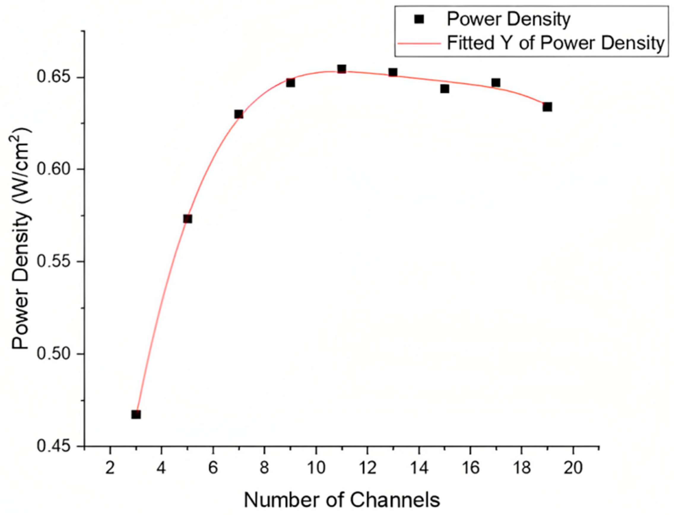
4.2. Geometry Variation Optimization Results

Figure 7, Figure 8 and Figure 9 demonstrate the optimisation of how different geometries affect the power density of the PEMFC. Moreover, they illustrate a clear optimum number of gas channels and spacing between those gas channels. The optimum number of channels was found to be 11, giving the cell the highest power density and, consequently, the highest power output. The channel spacing for this set of channels was 3.25 mm.

In Figure 8, the console shows most of the reaction taking place towards the inlet side of the serpentine channels. The higher the current density, the more hydrogen-oxygen reaction takes place at that location on the PEM surface. This is likely to be due to the oxygen reacting and running out as it is depleted due to the PEMFC being cathode dependent, as discussed previously. The oxygen depletion for the 11-channel configuration is shown in Figure 10. The current density is higher where the cathode gas channels are located, especially close to the inlet of the cathode. Figure 9 shows the power density increasing slightly with channel spacing at the beginning, reaching a maximum point and then decreasing with higher channel spacing. This is likely due to the higher current density close to the inlet of the cathode, where more hydrogen-oxygen reactions can occur.

At a lower spacing of the channels, this initial high level of reaction can spread further across the cell. This means a higher overall current density, as there is more oxygen to react before being depleted, close to the cathode inlet. In higher channel spacing geometry configurations, after the maximum point, the power density decreases are likely to be due to fewer gas channels, which means that there is less reaction occurring, as there is less area for the reactants to come into contact with the catalyst and react for both the anode and cathode reactants. To apply this to any PEMFC, the ratio between channel width, serpentine channel height (in this case, 47.5 mm as shown in Figure 1 and in the final model), and channel spacing can likely be used. The value is 1:2.6:38, respectively, to maximize the power output of PEMFC with the same control variables, including an operation pressure of 175,000 Pa, an operation temperature of 300.15 K, and inlet velocities of 0.064 m/s and 0.896 m/s for the anode and cathode, respectively.

4.3. Filleting Results and Final Design

Figure 11 shows the power density plotted against the radius of the fillet. It shows that the higher the fillet radius, the lower the power density of the fuel cell. The graph shows a small increase in power density after the initial decrease, and this could be due to the 90-degree angle turns in the geometry slowing down the flow of oxygen around the cell. However, this is outweighed by the potential of covering more cell area with a lower to no fillet radius, increasing the overall current flux and power output of the cell at 0.3 V. Figure 12 shows how, at the cathode inlet, oxygen gas can flow further into the cell than without a fillet. This is further supported by

Table 9. Power density of 19-channel configuration filleted vs. not filleted.

Fillet Radius (mm)	Power Density (W/cm2)
0	0.6338817
0.75	0.6341631

, where the less powerful 19-channel configuration is given a fillet of 0.75 mm, which increases the cell’s power output. Figure 11 shows that the higher the fillet radius in general, the lower the cell’s power output due to the less active area covered by the cathode channels. Therefore, the best gas channel configuration and the final design of this research is the 11-channel configuration, as shown in Figure 13.

5. Conclusions

In this research, the PEMFC model results follow the trends of the experimental results from the literature closely. The numerical values of the validation model were similar but not the same as the experimental results from the case study model, even though the model used the same boundary conditions. This is likely due to the many conditions of the model not being specified in the study literature, due to using different software to model. This includes flow courant number, which variables used BCGSTAB, and the order of the method used. In addition, as discussed in validation model boundary conditions and Setup Section 3.3, the mass flow rates and pressure boundary conditions differed from the case study and can affect the results’ validity. However, the trends between the models and experimental results are the same, and the model is sufficiently valid to satisfy the purposes of this research. The most relevant findings can be drawn as follows:

• The optimum power output voltage was found to be 0.3 V for a 25 cm² active area. This can be applied to any PEMFC by extrapolating a 1 volt of potential difference for every 83.3 cm² active area.
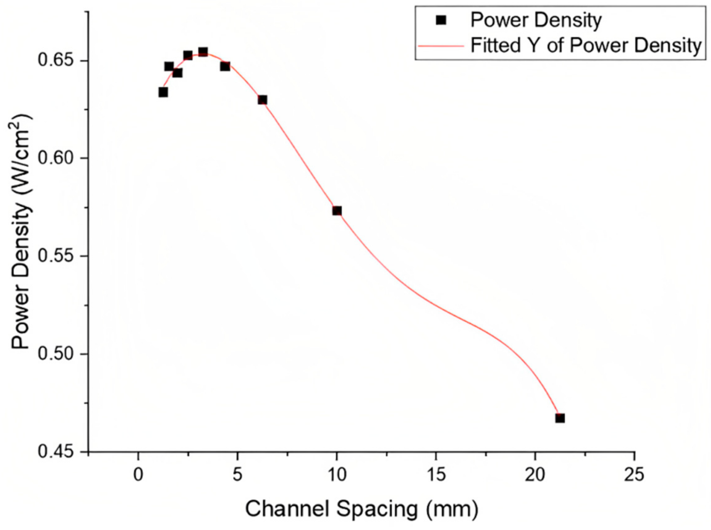
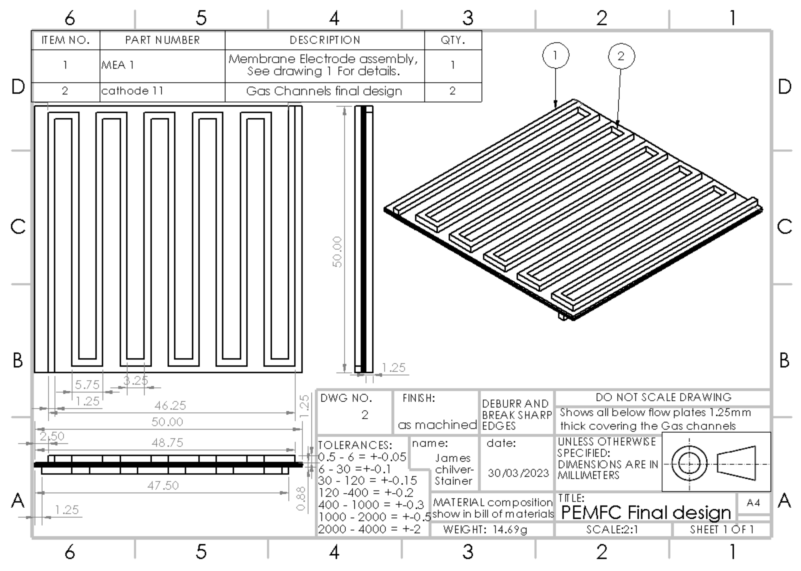
• The optimum configuration was determined to have 11 gas channels with a spacing of 3.25 mm, giving a channel width to channel spacing to serpentine channel length ratio of 1:2.6:38 for any PEMFC with a pressure of 175,000 Pa, an operation temperature of 300.15 K, and inlet velocities of 0.064 m/s and 0.896 m/s for the anode and cathode, respectively.
• Further research is required both to validate this ratio over a range of PEMFC sizes with different active areas, and experiments need to be conducted using a PEMFC to properly validate these results with real-life data so that they can be used in fuel cells in the future.
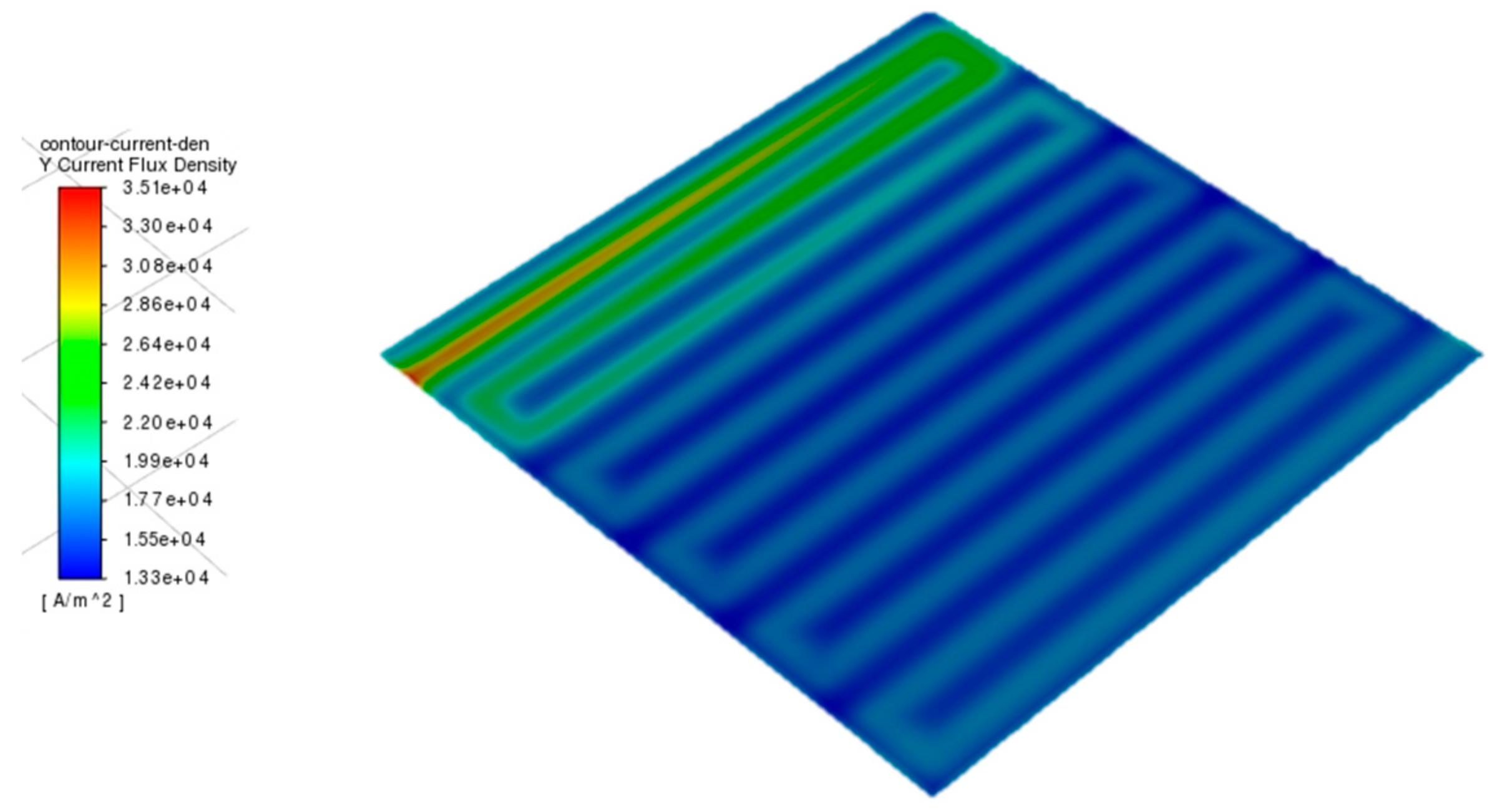
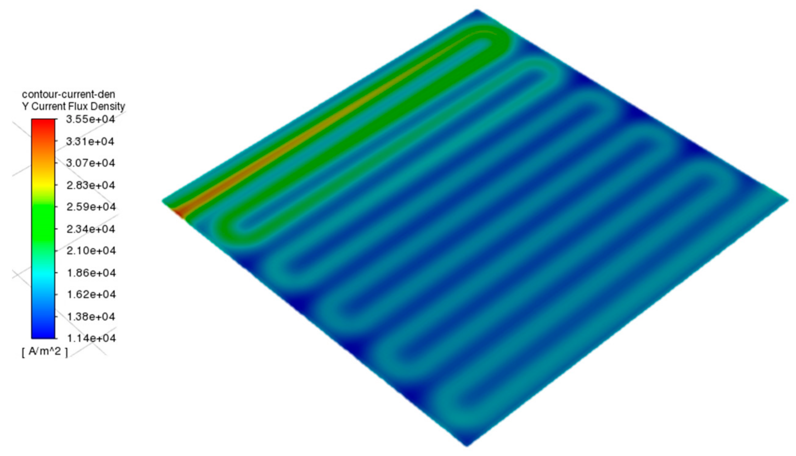
• The optimum 3.25 mm channel spacing is likely due to the combination of a high initial oxygen spread before being depleted, producing current flux and power. Additionally, it could be due to the increased area covered by having more channels.
• There is scope for further improvement in the modelling. There is a possibility of having an increased space close to the inlet of the cathode and a lower spacing further away from the inlet close to the outlet. This would mean that the initial oxygen can spread across the cell faster and have the increased area covered close to the outlet. According to the results of this study, there is potential to increase the power output of the cell further.
• According to the results, fillets to the bends of the serpentine channels decrease the power output for the 11-gas channel configuration due to the less active area covered by the serpentine channels.

These accurate models of 3D PEMFC Serpentine Gas Channel Fluid Flow results could be used to find the optimum serpentine gas channel configuration for any PEMFC with the same control variables, and with further research, for any set of control variables. This would be especially useful for increasing the acceleration of HPV’s and their fuel use capabilities. It could also potentially mean less fuel cell stacks would be needed to power an HPV, saving material costs and reducing carbon emissions when manufacturing HPVs.

Future research in this area should focus on validating the results of this study through experimentation, particularly with different PEMFC sizes and active areas. Additionally, there is scope for further optimisation of the gas flow channel configuration to improve power output even further. In particular, exploring the potential benefits of fillets at the inlet and outlet of the cathode channels could lead to significant improvements. Furthermore, the findings of this study can be extended to explore the impact of gas channel configuration on other fuel cell technologies, such as solid oxide fuel cells (SOFCs) and alkaline fuel cells (AFCs). Such investigations could pave the way for even more efficient and cost-effective fuel cell technologies, making them more accessible and widespread in various applications.

References

1. Balasankar, A.; Arthiya, S.E.; Ramasundaram, S.; Sumathi, P.; Arokiyaraj, S.; Oh, T.; Aruchamy, K.; Sriram, G.; Kurkuri, M.D. Recent Advances in the Preparation and Performance of Porous Titanium-Based Anode Materials for Sodium-Ion Batteries. Energies 2022, 15, 9495. [Google Scholar] [CrossRef]
2. Liu, X.; Reddi, K.; Elgowainy, A.; Lohse-Busch, H.; Wang, M.; Rustagi, N. Comparison of well-to-wheels energy use and emissions of a hydrogen fuel cell electric vehicle relative to a conventional gasoline-powered internal combustion engine vehicle. Int. J. Hydrog. Energy 2020, 45, 972–983. [Google Scholar] [CrossRef]
3. Shusheng, X.; Qiujie, S.; Baosheng, G.; Encong, Z.; Zhankuan, W. Research and development of on-board hydrogen-producing fuel cell vehicles. Int. J. Hydrog. Energy 2020, 45, 17844–17857. [Google Scholar] [CrossRef]
4. Zhang, X.; Ma, X.; Shuai, S.; Qin, Y.; Yang, J. Effect of micro-porous layer on PEM fuel cells performance: Considering the spatially variable properties. Int. J. Heat Mass Transf. 2021, 178, 121592. [Google Scholar] [CrossRef]
5. Collier, A.; Wang, H.; Yuan, X.Z.; Zhang, J.; Wilkinson, D.P. Degradation of polymer electrolyte membranes. Int. J. Hydrog. Energy 2006, 31, 1838–1854. [Google Scholar] [CrossRef]
6. Tang, H.; Wang, S.; Pan, M.; Yuan, R. Porosity-graded micro-porous layers for polymer electrolyte membrane fuel cells. J. Power Sources 2007, 166, 41–46. [Google Scholar] [CrossRef]
7. Trogadas, P.; Parrondo, J.; Ramani, V. Degradation Mitigation in Polymer Electrolyte Membranes Using Cerium Oxide as a Regenerative Free-Radical Scavenger. Electrochem. Solid State Lett. 2008, 11, B113–B116. [Google Scholar] [CrossRef]
8. Kim, H.-Y.; Kim, K. Numerical study on the effects of gas humidity on proton-exchange membrane fuel cell performance. Int. J. Hydrog. Energy 2016, 41, 11776–11783. [Google Scholar] [CrossRef]
9. Marappan, M.; Narayanan, R.; Manoharan, K.; Vijayakrishnan, M.K.; Palaniswamy, K.; Karazhanov, S.; Sundaram, S. Scaling up Studies on PEMFC Using a Modified Serpentine Flow Field Incorporating Porous Sponge Inserts to Observe Water Molecules. Molecules 2021, 26, 286. [Google Scholar] [CrossRef]
10. Hashemi, F.; Rowshanzamir, S.; Rezakazemi, M. CFD simulation of PEM fuel cell performance: Effect of straight and serpentine flow fields. Math. Comput. Model. 2012, 55, 1540–1557. [Google Scholar] [CrossRef]
11. Krastev, V.; Falcucci, G.; Jannelli, E.; Minutillo, M.; Cozzolino, R. 3D CFD modeling and experimental characterization of HT PEM fuel cells at different anode gas compositions. Int. J. Hydrog. Energy 2014, 39, 21663–21672. [Google Scholar] [CrossRef]
12. Yuan, L.; Jin, Z.; Yang, P.; Yang, Y.; Wang, D.; Chen, X. Numerical Analysis of the Influence of Different Flow Patterns on Power and Reactant Transmission in Tubular-Shaped PEMFC. Energies 2021, 14, 2127. [Google Scholar] [CrossRef]
13. Kahraman, H.; Orhan, M.F. Flow field bipolar plates in a proton exchange membrane fuel cell: Analysis & modeling. Energy Convers. Manag. 2017, 133, 363–384. [Google Scholar]
14. Canonsburg, T.D. Ansys Fluent Fuel Cell Modules Manual, Knowl. Creat. Diffus. Util. 2012, 15317, 724–746. [Google Scholar]
15. D’adamo, A.; Riccardi, M.; Borghi, M.; Fontanesi, S. CFD Modelling of a Hydrogen/Air PEM Fuel Cell with a Serpentine Gas Distributor. Processes 2021, 9, 564. [Google Scholar] [CrossRef]
16. Tian, P.; Liu, X.; Luo, K.; Li, H.; Wang, Y. Deep learning from three-dimensional multiphysics simulation in operational optimization and control of polymer electrolyte membrane fuel cell for maximum power. Appl. Energy 2021, 288, 116632. [Google Scholar] [CrossRef]
17. Varghese, G.; Venkatesh Babu, K.P.; Joseph, T.V.; Chippar, P. Combined effect of channel to rib width ratio and gas diffusion layer deformation on high temperature—Polymer electrolyte membrane fuel cell performance. Int. J. Hydrog. Energy 2022, 47, 33014–33026. [Google Scholar] [CrossRef]
18. Sapkota, P.; Brockbank, P.; Aguey-Zinsou, K.-F. Development of self-breathing polymer electrolyte membrane fuel cell stack with cylindrical cells. Int. J. Hydrog. Energy 2022, 47, 23833–23844. [Google Scholar] [CrossRef]
19. Wang, Y.; Wang, X.; Fan, Y.; He, W.; Guan, J.; Wang, X. Numerical Investigation of Tapered Flow Field Configurations for Enhanced Polymer Electrolyte Membrane Fuel Cell Performance. Appl. Energy 2022, 306, 118021. [Google Scholar] [CrossRef]
20. Su, G.; Yang, D.; Xiao, Q.; Dai, H.; Zhang, C. Effects of vortexes in feed header on air flow distribution of PEMFC stack: CFD simulation and optimization for better uniformity. Renew. Energy 2021, 173, 498–506. [Google Scholar] [CrossRef]
21. Cao, Y.; El-Shorbagy, M.; Dahari, M.; Cao, D.N.; El Din, E.M.T.; Huynh, P.H.; Wae-Hayee, M. Examining the relationship between gas channel dimensions of a polymer electrolyte membrane fuel cell with two-phase flow dynamics in a flooding situation using the volume of fluid method. Energy Rep. 2022, 8, 9420–9430. [Google Scholar] [CrossRef]
22. Yuan, H.; Dai, Y.; Li, H.; Wang, Y. Modeling of high-temperature polymer electrolyte membrane fuel cell for reaction spatial variation. Int. J. Heat Mass Transf. 2022, 195, 23209. [Google Scholar] [CrossRef]
23. Huang, F.; Qiu, D.; Peng, L.; Lai, X. Optimization of entrance geometry and analysis of fluid distribution in manifold for high-power proton exchange membrane fuel cell stacks. Int. J. Hydrog. Energy 2022, 47, 22180–22191. [Google Scholar] [CrossRef]
24. Yun, S.-H.; Woo, J.-J.; Seo, S.-J.; Yang, T.-H.; Moon, S.-H. Estimation of approximate activation energy loss and mass transfer coefficient from a polarization curve of a polymer electrolyte fuel cell. Korean J. Chem. Eng. 2012, 29, 1158–1162. [Google Scholar] [CrossRef]
25. Versteeg, H.K.; Malalasekera, W. An Introduction to Computational Fluid Dynamics: The Finite Volume Method. Available online: http://ftp.demec.ufpr.br/disciplinas/TM702/Versteeg_Malalasekera_2ed.pdf (accessed on 22 April 2023).
Figure 1. Initial Model Geometry.
Energies 16 03722 g001
Figure 2. Mesh dependency analysis: Number of cells in mesh plotted against current density.
Energies 16 03722 g002
Figure 3. Final model mesh with the scale inflation and sweep methods.
Energies 16 03722 g003
Figure 4. Polarization (solid lines)/Power density curve (dashed lines) compared with [15].
Energies 16 03722 g004
Figure 5. Initial model potential difference from anode to cathode and power density curves plotted against current density.
Energies 16 03722 g005
Figure 6. Validation model potential difference from anode to cathode and power density curves plotted against current density with optimum power output points labelled.
Energies 16 03722 g006
Figure 7. Optimisation of the number of gas channels by recording the power density of each geometry run.
Energies 16 03722 g007
Figure 8. Current flux density contour across optimum 11 channel configuration PEM.
Energies 16 03722 g008
Figure 9. Optimisation of channel spacing from the different number of gas channel geometry configurations by recording power density.
Energies 16 03722 g009
Figure 10. Oxygen mass fraction cathode 11 gas channel configuration.
Energies 16 03722 g010
Figure 11. Optimisation of fillet radius of 11-channel PEMFC recording power density.
Energies 16 03722 g011
Figure 12. Current flux density contour for 1.625 mm fillets.
Energies 16 03722 g012
Figure 13. Final 11-channel configuration of the research.
Energies 16 03722 g013