Article

An Offshore Solar Irradiance Calculator (OSIC) Applied to Photovoltaic Tracking Systems

Institute for Sustainable Energy, University of Malta, MXK 1531 Marsaxlokk, Malta
*
Author to whom correspondence should be addressed.
Energies 2023, 16(9), 3735; https://doi.org/10.3390/en16093735
Submission received: 13 February 2023 / Revised: 25 April 2023 / Accepted: 25 April 2023 / Published: 27 April 2023
(This article belongs to the Section A2: Solar Energy and Photovoltaic Systems)

Abstract

:
Offshore photovoltaic installations are the future technology in solar energy since they enable the use of the large amount of maritime space, which is especially important when land space is not available. Various research groups are working to create viable installations. However, there are currently no tools available that an offshore system designer can use to quantify the effect of wave response motion on offshore photovoltaic installations. This research presents a new simulation tool termed the Offshore Solar Irradiance Calculator (OSIC) that is able to quantify this effect. Furthermore, a yearly parametric analysis is presented to show the effects of a characteristic wave equation on different offshore tracking systems; namely, horizontal single-axis tracking, vertical single-axis tracking and dual-axis tracking. Finally, another parametric analysis is presented to show the effects of varying wave amplitudes of oscillations on the incident irradiance received by these tracking systems.

1. Introduction

A tracking system involves changing a PV system’s tilt, orientation or both in order to maximise the incident solar radiation throughout the day. This can be achieved in various different ways, which can be categorised as passive [1] or active trackers. Passive trackers usually use containers filled with a low-boiling-point liquid that, when heated by incident solar radiation, expands into a gas and pushes the rest of the liquid to a shaded part of the container. This shift in weight results in the rotation of the solar panel until the fluid reaches thermal equilibrium and, hence, the rotation stops [2,3]. When compared to non-tracking systems, passive trackers have been reported to achieve up to 23.3% increases in power output [4] and 23% increases in efficiency [5]. Although passive tracking can be cheap to implement and maintain, it is sensitive to weather conditions, such as low temperatures, radiation and high wind speeds [2].
Active tracking systems involve the use of geared motors, sensors and control algorithms to detect and follow the Sun’s position during the day. Active photovoltaic trackers can achieve higher gains than passive trackers but usually come at a higher installation cost and may require more maintenance due to the increased number and complexity of components. These trackers have been classified into various categories; however, the most common are single-axis and dual-axis solar trackers [6]. Single-axis tracking can employ a horizontal axis parallel to the ground (horizontal single-axis trackers (HSATs)), a tilted axis with horizontal tracking (HTSATs), a vertical axis normal to the ground (vertical single-axis trackers (VSATs)) or a polar axis aligned with the polar star (PASATs) [7]. In one study [8], it was found that HSATs are more suitable for low-latitude regions and can achieve annual energy gains of 16% to 24% when the axis is oriented south–north. A similar study [9] concluded that VSATs are more suitable in regions with abundant solar resources, where the collectible solar radiation can be increased by up to 28%. Another study [10] reported an energy yield gain of 15.4% when comparing an HSAT with a non-tracking installation.
Dual-axis trackers are the most complex to implement but can achieve the greatest energy gains. These trackers have two axes, usually perpendicular to each other, with one axis adjusting the tilt of the solar panels while the other axis adjusts the azimuth. This tracking configuration can be controlled by either an open-loop or a closed-loop control system. In an open-loop control system, the control algorithm is programmed to make certain fixed movements throughout the day based on weather data and irradiance models. The accuracy of this type of control is highly dependent on the quality of the data on which the programming is based. In contrast, closed-loop tracking systems use sensors, such as light-dependent resistors (LDRs), to obtain feedback on irradiance intensity. Based on this feedback, the tilt and azimuth of the solar panel are adjusted until peak intensity is reached. Closed-loop tracking systems can track the Sun’s position very accurately and are mostly limited by the feedback sensor’s accuracy. Sebastijan et al. [11] designed and tested an open-loop dual-axis solar tracker and achieved an increase in energy yield of 27% when compared to non-tracking PV installations. Moreover, a closed-loop dual-axis solar tracking system was reported to increase daily energy yield by 39.43% [12]. Although these trackers can result in considerable increases in efficiency, they require higher maintenance and are susceptible to major forces due to the weight of the panels and the effect of wind when the panels are at a high tilt angle [7].
Offshore tracking must overcome various challenges to become a mature and viable technology. Firstly, active tracking algorithms find it difficult to accurately follow the Sun while the raft underneath is moving due to incoming waves. Furthermore, once the algorithm successfully tracks the Sun, any movement caused by the response of the floating raft to incoming waves results in a change in the amount of incident radiation on the photovoltaic panels. This movement can have a positive or negative effect depending on the type of tracking system implemented. For example, any movement affecting an accurate dual-axis tracking algorithm should result in the photovoltaic panels receiving less irradiance when compared to the same tracking system installed on land. However, this effect has not been quantified in the literature. Therefore, the aim of this study was to optimise the simulation tool presented in a previous publication [13] and to parametrically analyse the effect of wave response motion on the incident irradiance on offshore tracking photovoltaic installations.

2. Materials and Methods

The simulation tool presented in this study was programmed using C language in Visual Studio 2022 Integrated Development Environment (IDE). The aim of this part of the research was to create user-friendly software that includes a graphical user interface (GUI) and is able to process inputs and output results in a fraction of the time it takes for the Excel-based tool [13]. Furthermore, N–S HSATs, VSATs and dual-axis tracking were added to the tool, making it the first tool (at the time of writing) that can calculate the effects of wave response motion on both non-tracking and tracking offshore photovoltaic installations.
The movement of the floating raft was divided into three parts; namely, pitch, yaw and roll. The OSIC software had to allow the user to use different orientations for the solar panels and the floating raft and it needed to automatically calculate the tilts and orientations of the solar panels without requiring third-party software. Therefore, rotational matrices were used in order to calculate new tilts and orientations after particular movements.

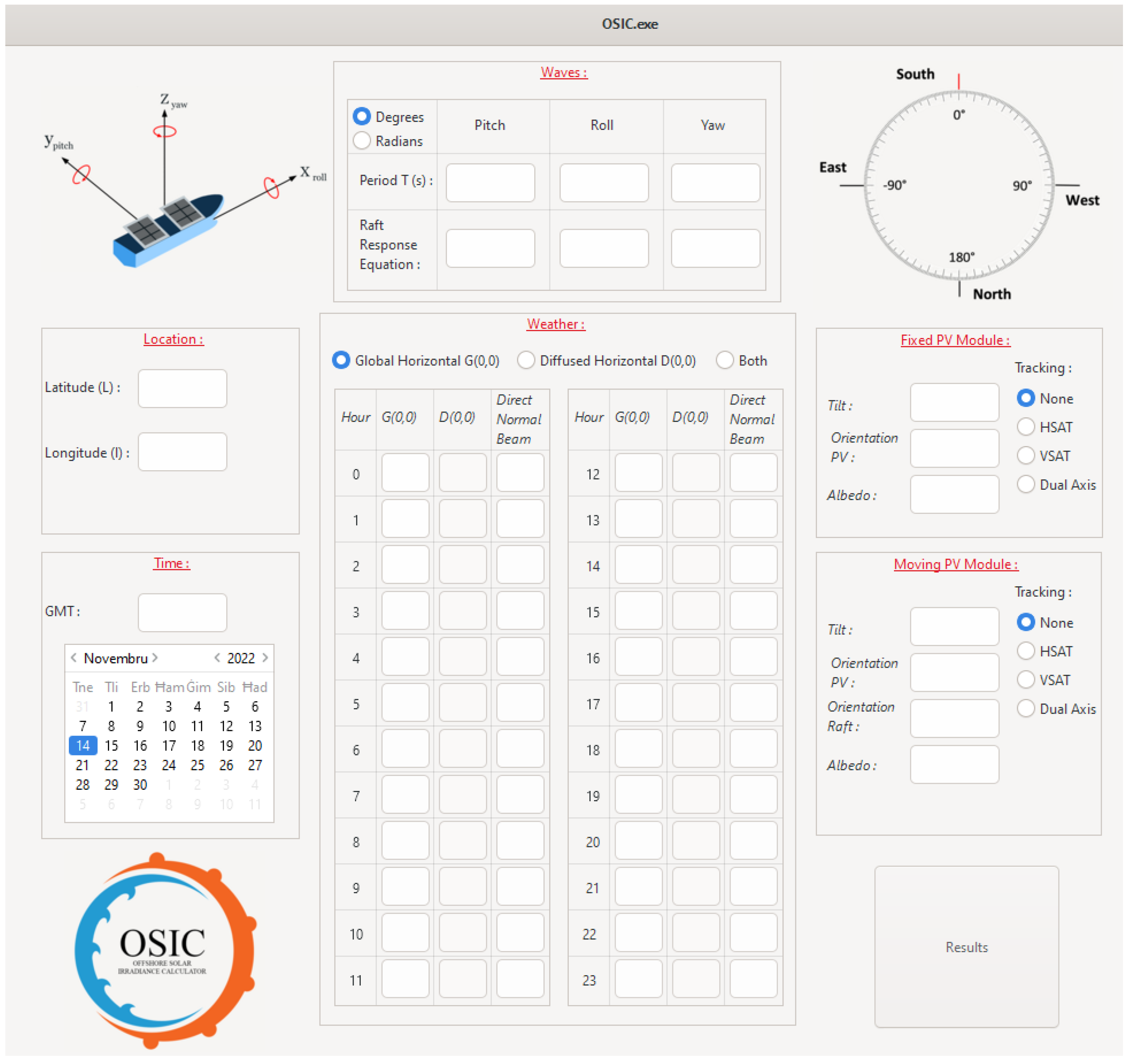
2.1. General Operation of OSIC

A graphical user interface (GUI) was created using the open-source GTK library [14]. Furthermore, an application called Glade [15] was used in order to facilitate the placement of widgets. In addition, the pbPlots library [16] was used for the interface to enable plotting graphs. Hence, the GUI was split into three sections; namely, the input section, the graphical results section and the numerical results section. Figure 1 shows the input section.
The user first has to input the longitude and latitude of the installation, the Greenwich Mean Time (GMT) and the date for which the simulation is to be run. The date is input by choosing the correct day and year from the calendar on the left-hand side of the user interface. This information is used by an NOAA calculator [17] to find the position of the Sun for every hour of the day. Hence, if the user selects a tracking system, the software will calculate the tilt and azimuth of the solar panels in accordance with the position of the Sun during the day. On the other hand, if the user selects a non-tracking installation, the tilt and azimuth will be fixed to the values entered by the user. Furthermore, the user has to enter hourly data for the direct normal beam and the global horizontal radiation G (0,0), diffused horizontal radiation D (0,0) or both. If the user enters only one of either the global or diffused radiation, the software will automatically calculate the other parameter.
Next, if a wave response movement is required, the user has to enter a characteristic equation for this movement under one of the three movement categories. In order for the software to be able to understand and compute this user input, a string-parsing method was used to allow the different parts of the equation to be read. When the user enters an equation, the program only records a series of characters and does not understand what each character means. Therefore, specific instructions related to each character had to be programmed so that, when the program reads each of these characters independently, it can understand it and apply the correct instruction. With this part of the code, the software is able to recognise various mathematical functions and symbols, such as trigonometric functions, f, t and pi. If a periodic equation is entered by the user, it has to be accompanied by an input for the period. Consequently, the software will compute the amplitudes resulting from these equations at a time step of 0.1 s until the period value is reached. The right-hand rule was used as a convention for movements, as shown in Figure 2, and users must adhere to this rule in order to obtain correct results.
After the user inputs the characteristic equations for pitch, yaw and roll movements, they must also choose between “Degrees” and “Radians” in order to inform the software how it should handle trigonometric functions. Finally, details must be input for the “Fixed PV Module” and the “Moving PV Module”. These details include the designed tilt and orientation of the PV for non-tracking installations, the albedo of the installation location and the orientation of the raft, which can be different from that of the solar panels. The “Orientation PV” refers to the azimuth of the PV installation, while the “Orientation Raft” refers to the orientation of the front of the raft, abiding with the convention shown in Figure 2. If dual-axis or HSAT tracking is selected, the “Tilt” and “Orientation PV” boxes will be greyed out and will not allow any input, while if VSAT is selected, only the “Orientation PV” box will be greyed out.
Data inputs are protected against unexpected entries in order to prevent the software from crashing. For example, if a user inputs a negative period for any of the wave equations, a pop-up window will prompt the user to fix this before continuing. Once all the required fields have been filled in, the user clicks on the “Results” button and the software runs all the calculations while the GUI changes to the graphical results section shown in Figure 3. This section is composed of six graphs, two for each raft movement. The top graphs show the irradiance incident on the fixed solar panels in blue and the irradiance incident on the offshore solar panels in orange. The second graph shows the percentage difference for the two irradiances when subtracting the values for the fixed panels from those for the moving panels. This means that a negative percentage difference indicates that the moving PV installation receives lower irradiance than the fixed installation.
Finally, the user has the option to click on the “Set Up” button, return to the GUI input section and modify some parameters or click on the “Details” button to view the GUI numerical results section. In this section, the numerical values for the irradiance for every hour for both fixed and moving PVs are shown. In addition, this section also displays the percentage difference for the irradiance of the moving and the fixed solar panels, following the same convention as the graphical results section. Moreover, both results sections are dynamic and only show hours with irradiance values above zero in order to minimize the number of calculations performed by the application and produce a cleaner GUI. The data presented in this section can be copied into third-party software for further processing and analysis. Finally, from this window, the user can return to either the graphical results section or the input section.
The OSIC simulation tool was extensively tested and any bugs that were discovered were corrected. The software robustness was increased by optimising any memory leaks occurring in the code and correctly handling unexpected user inputs without crashing. Furthermore, the software is able to check for erroneous weather data and a pop-up message is shown to the user, prompting them to continue or to modify the input parameters. Finally, information messages are shown when the pointer moves over various parts of the software in order to better guide the user.

2.2. Calculation of Tilt and Azimuth after Movement
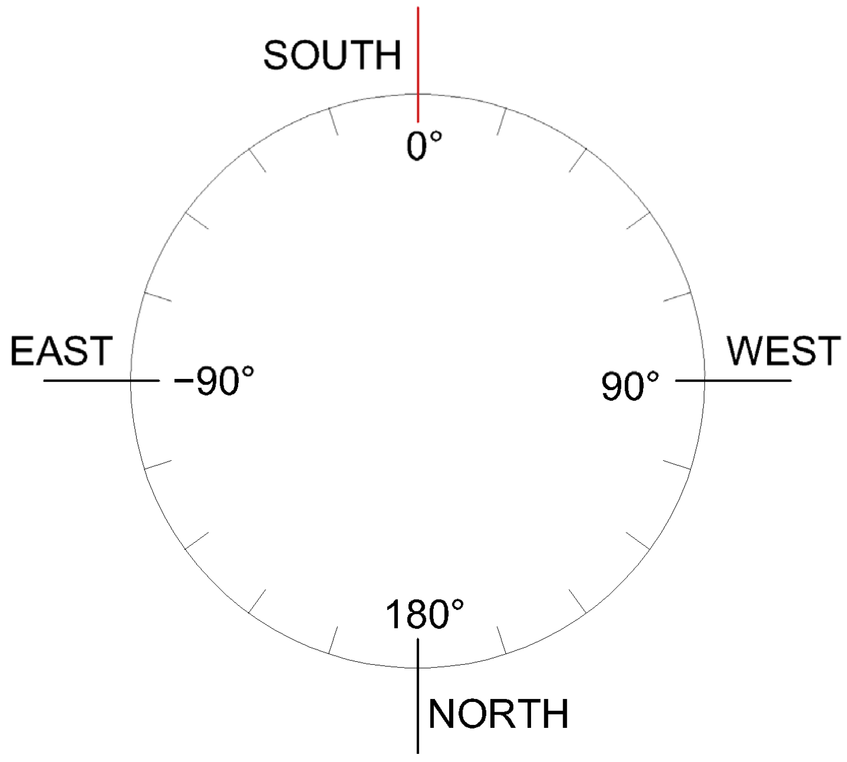
In order to determine the incident radiation for each wave-induced movement, it is necessary to know the exact tilt and azimuth of the offshore solar panels. These new tilts and azimuths are calculated every 0.1 s during a given period. However, it is not necessary to recalculate them every hour since the wave response equations for the raft are assumed to be the same throughout the day. In order to calculate the new tilt and azimuth, a number of conventions had to be used. Firstly, the orthonormal frame of reference in which the boat is located follows the right-hand rule, as defined in Figure 2. In this figure, the red arrow indicates the positive direction of rotation. For example, for the yaw, if the raft is turning clockwise, the angle will be considered negative. The orthonormal reference is composed of the three vectors defined in Equation (1).
x = ( 1 0 0 ) ;   y = ( 0 1 0 ) ;   z = ( 0 0 1 )
To calculate the rotations made by the solar panel, rotation matrices must be used. Rotation matrices calculate the new object position after a rotation around one of the three main axes passing through the origin of the orthonormal reference frame in which this object is located (represented in Figure 2 by the x, y and z axes). These new positions are then defined with reference to the basic orthonormal reference frame. It is possible to define rotation matrices both clockwise and counter-clockwise; however, OSIC software uses the clockwise matrix of rotation. The three rotation matrices for the pitch, yaw and roll movements are defined in Equations (2)–(4), respectively.
R p i t c h = cos x 0 sin x 0 1 0 sin x 0 cos x
R y a w = cos x sin x 0 sin x cos x 0 0 0 1
R r o l l = 1 0 0 0 cos x sin x 0 sin x cos x
It is assumed that:
-
The vector x in front of the raft is oriented south;
-
The orientation of the PV module is the same as that of the raft;
-
The tilt of the panel is 0°; that is, it is lying horizontally on the raft.
Hence, a vector a normal to the plane formed by the solar panel is defined in Equation (5).
a = 0 0 1
When an object performs several rotations, it is possible to combine rotation matrices to create a new rotation matrix that describes the complete set of rotations. Hence, this new combined rotation matrix is multiplied by the normal vector of the base solar panel to obtain the new normal vector of the solar panel after it has undergone a set of rotations. When a photovoltaic installation is installed on a floating raft, its orientation may be different from that of the raft. This means that if we take the raft’s orientation as a reference, a rotation around the z-axis (yaw) must be performed in order to describe the orientation of the PV. If the angle between the orientation of the PV and the orientation of the raft is ψ , then this rotation can be described by the rotation matrix A defined by Equation (6).
A = cos ψ sin ψ 0 sin ψ cos ψ 0 0 0 1
Once this rotation is complete, the main orthonormal frame may be different from the PV module’s orthonormal frame. It is then possible to perform an extrinsic rotation around one of the axes of the main frame or an intrinsic rotation around one of the axes of the new PV frame itself. After the rotation to match the orientation of the PV panel (described by matrix A), it is necessary to perform an intrinsic rotation to achieve the designed tilt of the PV panel. For this purpose, a rotation around the y-axis of the orthonormal reference frame of the PV panel is performed. If θ represents the angle of this rotation, the matrix B describing this rotation is given by Equation (7). This matrix is then multiplied by matrix A to obtain the rotation matrix C defined by Equation (8). This rotation matrix is used as the basis for calculating the three rotation matrices for the roll, pitch and yaw effects of the waves on the raft.
B = cos θ 0 sin θ 0 1 0 sin θ 0 cos θ
C = A · B = cos ψ cos θ sin ψ cos ψ sin θ sin ψ cos θ cos ψ sin ψ sin θ sin θ 0 cos θ
To calculate the effect of the roll on the position of the solar panel, the rotation matrix of the roll must be used. This is an extrinsic rotation because the effect of the waves is linked to the position of the raft and not that of the solar panel; therefore, the main orthonormal reference frame must be used. If ϕ represents the angle of this rotation, the matrix D describing a roll movement is defined by Equation (9). This matrix is then multiplied by matrix C in order to obtain a new combined matrix E, as shown in Equation (10).
D = 1 0 0 0 cos ϕ sin ϕ 0 sin ϕ cos ϕ
E = D · C = cos ψ cos θ sin ψ cos ψ sin θ cos ϕ sin ψ cos θ + sin ϕ sin θ cos ϕ cos ψ cos ϕ sin ψ sin θ sin ϕ cos θ sin ϕ sin ψ cos θ cos ϕ sin θ sin ϕ cos ψ sin ϕ sin ψ sin θ + cos ϕ cos θ
Hence, the next step is to calculate the normal vector to the solar panel v after it has undergone the roll effect. This is achieved by multiplying the normal vector of the solar panel before rotation, a , by the matrix E, as shown in Equation (11).
v = E a = cos ψ sin θ cos ϕ sin ψ sin θ sin ϕ cos θ sin ϕ sin ψ sin θ + cos ϕ cos θ
The next calculation determines the new tilt angle of the solar panel after the roll movement (βn), which corresponds to the angle between the vector v and the plane of the flat solar panel; it is given by Equation (12).
β n = 90 a r c s i n sin ϕ sin ψ sin θ + cos ϕ cos θ cos ψ sin θ 2 + cos ϕ sin ψ sin θ sin ϕ cos θ 2 + sin ϕ sin ψ sin θ + cos ϕ cos θ 2
To calculate the orientation of the solar panel after the roll movement, the angle, α, between the vector x = ( 1 0 0 ) and the projection of the vector v on the plane composed of the vectors x and y must be calculated. The projection of the vector v is given by Equation (13), while the angle α is calculated using Equation (14).
v ^ = p r o j v x + p r o j v y = cos ψ sin θ cos ϕ sin ψ sin θ sin ϕ cos θ 0
α = a r c o s cos ψ sin θ cos ψ sin θ 2 + cos ϕ sin ψ sin θ sin ϕ cos θ 2
However, the result for α is an unsigned angle that does not necessarily show the correct orientation, abiding by the convention shown in Figure 4. In order to obtain more information on the sign of α , the angle between the projection v ^ and the vector y = ( 0 1 0 ) is calculated using Equation (15). If this angle, σ, is between 0 and 90, then α will be negative; otherwise, it will be positive. Finally, the orientation of the raft as inputted by the user is added and the result is the true azimuth of the solar panel after a particular movement.
σ = a r c o s cos ϕ sin ψ sin θ sin ϕ cos θ cos ψ sin θ 2 + cos ϕ sin ψ sin θ sin ϕ cos θ 2
The calculations above give the tilt and azimuth of the solar panel after a roll movement. To obtain the tilt and azimuth after a yaw or a pitch movement, it is necessary to replace the matrix D in Equation (9) with other matrices. Matrix F in Equation (16) must be used for yaw movements, where τ is the angular amplitude. Likewise, matrix G in Equation (17) must be used for pitch movements, where n is the angular amplitude.
F = cos τ sin τ 0 sin τ cos τ 0 0 0 1
G = cos n 0 sin n 0 1 0 sin n 0 cos n

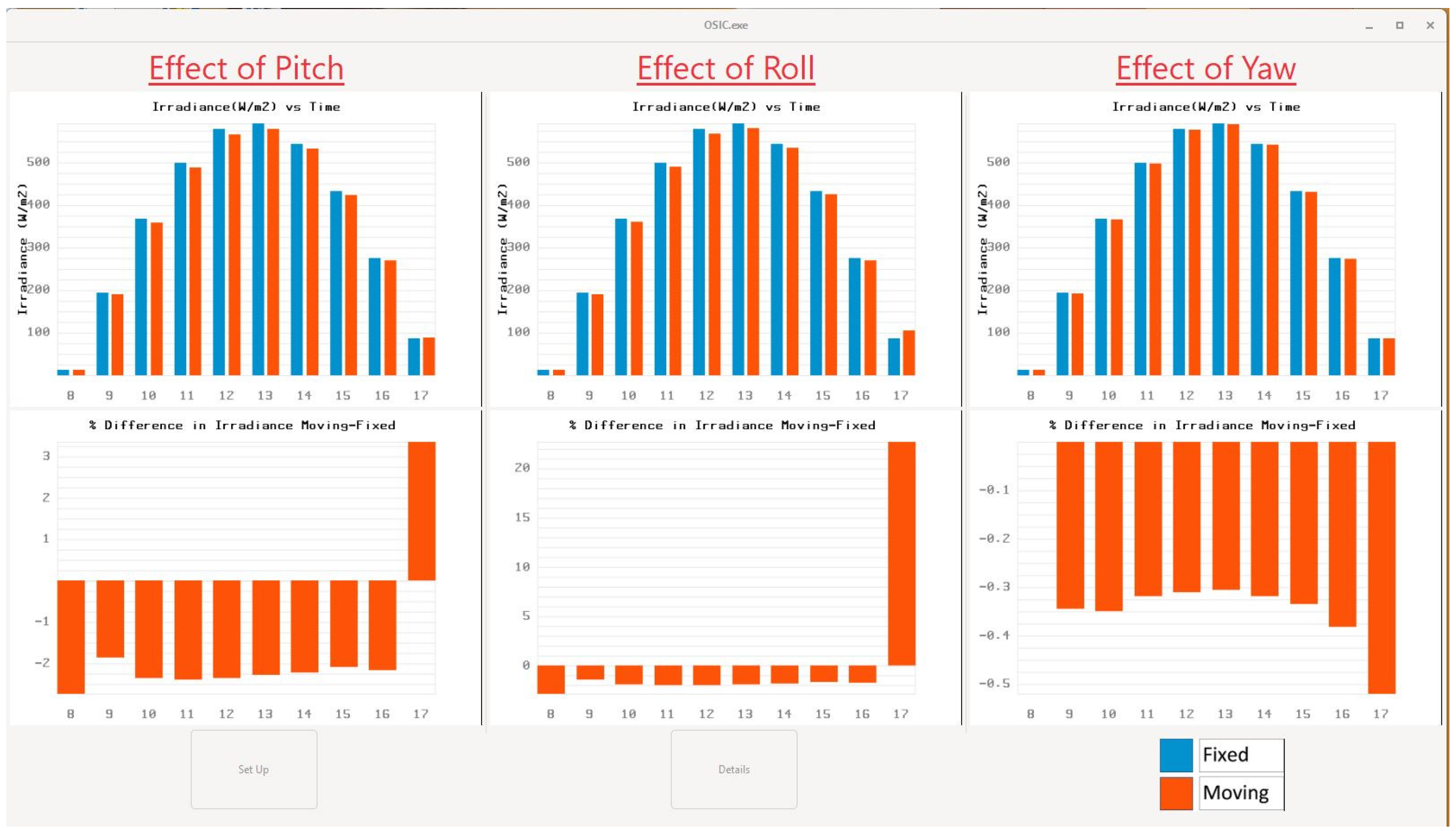
2.3. Calculation of Irradiance on Tracking Surface

When calculating the irradiance on a tracking surface, the anisotropic model—specifically, the Perez model—is used [18,19], which is similar to that described by Bugeja et al. [13]. A dual-axis tracker adjusts both the tilt and azimuth of the solar panel in order to ensure its surface is always perpendicular to the Sun throughout the day [20]. This implies that the tilt angle of the solar panel is always equal to the solar zenith angle, while the azimuth of the solar panel is always equal to the solar azimuth. A vertical single-axis solar tracker (VSAT) has a fixed tilt set during the installations, while its azimuth changes during the day and is equal to the solar azimuth. The incidence angle is determined by subtracting the surface’s fixed tilt from the solar zenith angle.
A horizontal N–S single-axis tracker (HSAT) tracks the Sun from east to west on a horizontal axis. This implies that the tilt constantly changes during the day, while the orientation is either towards the east or west. The solar panel’s tilt angle is a function of the solar azimuth angle γ S and the solar altitude α S given by Equation (18). The solar incident angle on the tilted surface, θ i , is determined using Equation (19) [20].
β n = tan 1 sin γ S tan α S
cos θ i = cos δ × sin ω 2 + cos cos ω + tan δ sin 2

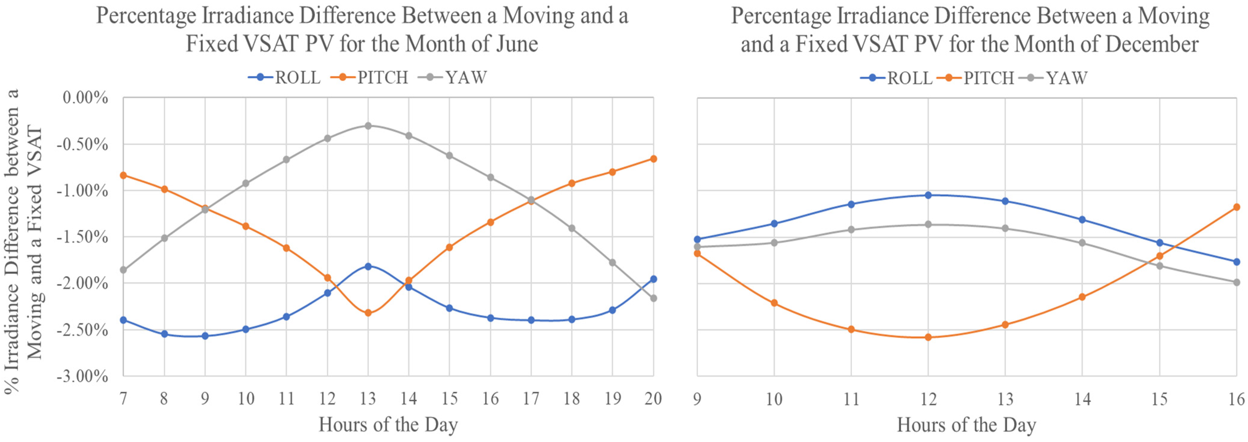
3. Results and Discussion

A parametric analysis was performed for all three different types of tracking systems and for each month of the year. A day was chosen for each month and weather data for that day were used in order to obtain the results. Clear days were chosen with the fewest clouds possible close to the 21st of each month in order to include equinoxes and solstices. Equation (20) was inputted for all three movements and a period of 6 s was chosen. The results obtained are shown in Table 1.
f t = 20 cos 2 π f t
The first observation from the results in Table 1 is that an HSAT system with an N–S horizontal axis and with the raft’s orientation facing south is more affected by roll movements than pitch and yaw movements. This is because yaw movements only change the azimuth of the PV, while pitch movements slightly change both the azimuth and tilt. In contrast, roll movements have a direct effect on the tilt of the PV, meaning that such movements go against the HSAT algorithm, which is designed to capture the maximum irradiance for such an installation. Therefore, OSIC software can inform a raft designer that, if such a tracking system is going to be installed, care must be taken to limit response movements to incoming waves in the roll direction. Figure 5 shows the hourly effects on an HSAT caused by roll, pitch and yaw movements for the months of June and December. Yaw movements have no effect on the HSAT system during the middle part of the day since the algorithm sets the PV to a horizontal inclination during this time. In contrast, pitch movements have a greater effect during this period since these movements result in a considerable change in tilt. Figure 6 shows the hourly effects on a VSAT caused by roll, pitch and yaw movements for the months of June and December. This figure clearly shows that yaw movements in December have a greater negative effect on the insolation than the same movements in June. This is because the irradiance on a tilted plane follows a cosine function. Therefore, although the change in incidence angle is actually lower in December than in June, the change in cos ( θ i ) is actually higher. This figure also shows that roll movements in mornings and evenings have a greater effect in summer than in winter. This is because, during these times of the day, roll movements have a major effect on the tilt of the solar panel. Since in summer the chosen tilt is close to the optimum, any deviation always results in a lower irradiance incident on the solar panel.
From the results in Table 1, it can be seen that yaw has a greater effect on dual-axis trackers than the other tracking mechanisms. This is because this tracking algorithm always orients the PV into a quasi-optimal tilt and orientation. Therefore, any movement will always result in a deviation from the optimum, which means a loss in the irradiance incident on the PV. Moreover, as seen in Figure 7, yaw movements on a dual-axis tracker have a higher negative impact in winter than other tracking systems, since tilts are higher and, therefore, changes in the azimuth have a greater effect on the incident radiation. Pitch movements in the mornings and evenings slightly alter the tilt and orientation and, therefore, do not have the same effect magnitude as roll movements. Although the effect of pitch movements increases in the middle of summer days since they start affecting the tilt, roll movements still have a considerable negative effect since, at these times, they vary both the tilt and orientation considerably. In contrast, at midday during winter, the panel is oriented towards a low-elevation Sun, which means it is at a high tilt. Therefore, roll movements are less important than pitch movements since the latter considerably affect the tilt, while the former slightly varies both the tilt and orientation.
A final parametric analysis was performed in order to observe the changes in the effects of waves with varying amplitudes of oscillations for a day in June. These amplitudes were varied between 0° and 50°. The results for dual-axis trackers and HSATs are shown in Figure 8 and Figure 9, respectively. Furthermore, three fixed tilts were chosen for the VSAT (namely, 5°, 30° and 50°) and the results are tabulated in Table 2. From these results, it can be seen that the relationship between the percentage difference in irradiance and the amplitude of oscillations is not linear for the chosen wave. Furthermore, roll effects are more predominant in tracking systems compared to the non-tracking systems previously published [13]. This is because, as previously discussed, roll movements in an HSAT directly influence the tilt of the PV, while roll movements for other tracking systems result in deviations in the tilt and orientation, both of which are quasi-optimised by the tracking algorithm.

4. Conclusions

This paper presented the optimisation of a simulation tool in order to include the effects of wave response motion on offshore HSAT, VSAT and dual-axis tracking photovoltaic systems. This new simulation tool was termed the Offshore Solar Irradiance Calculator (OSIC) and, at the time of writing, it is the only available tool that allows the user to quantify the effect of waves on offshore photovoltaic installations. A parametric analysis was performed using a characteristic wave equation and the effects of pitch, roll and yaw movements were observed and presented. Roll movements resulted in the maximum negative effects, with HSATs and VSATs demonstrating a maximum loss of −2.38%, while the dual-axis tracker demonstrated a loss of −2.3%. Furthermore, a parametric analysis of the effects of different wave-response amplitudes on the incident irradiance was presented. The greatest effect was observed for a 50° amplitude wave response, with losses exceeding −12%. Moreover, this research showed that, for the same wave type, the effect of a moving raft varies for non-tracking and tracking installations. The limitation of this study was that it assumed movement after the tracking algorithm successfully reached its objective. In reality, it is hypothesised that there will be other challenges in implementing offshore tracking since the tracking algorithm has to work in a constantly moving environment. Furthermore, the effect of shading caused by the movement of the floating raft was not quantified in this study. Moreover, the same characteristic wave response equation was used for the one-year simulation in order to be able to compare the results. In reality, the response amplitude varies during the year and, therefore, the effect on the incident radiation also varies accordingly. Similarly, the same albedo was used for land and offshore installations so as to isolate the effect caused by wave response motion. The difference in albedo between installations has a further effect on the incident radiation.

Author Contributions

Conceptualization, R.B.; methodology, R.B., L.D.; software programming, L.D., R.B.; software testing, R.B., L.D.; validation, R.B.; formal analysis, R.B., L.M.S.; investigation, R.B., L.D.; resources, L.M.S.; writing—original draft preparation, R.B.; writing—review and editing, L.M.S., L.D.; supervision, L.M.S.; project administration, L.M.S. All authors have read and agreed to the published version of the manuscript.

Funding

This research received no external funding.

Data Availability Statement

The data and software presented in this study are available on request from the corresponding author. The data are not publicly available due to ongoing work towards a PhD award. The software is not publicly available due to licensing agreements currently being drafted.

Conflicts of Interest

The authors declare no conflict of interest. The funders had no role in the design of the study; in the collection, analyses, or interpretation of data; in the writing of the manuscript; or in the decision to publish the results.

Nomenclature

AbbreviationDescription
ψ Angle between the orientation of the PV and the orientation of the raft
θAngle of rotation around the y-axis of the orthonormal reference frame of the PV panel
ϕAngle of rotation around the main orthonormal frame
βnNew PV tilt angle following a wave response movement
σ PV azimuth following a wave response movement
x, τ , nAngular amplitudes of roll, yaw and pitch movements
θ i Solar incident angle on tilted surface
δ Solar declination angle
ω Hour angle
γ S Solar azimuth angle
α S Solar altitude
fWave response frequency
tTime base

References

  1. Gevorkian, P. Alternative Energy Systems in Building Design; McGraw-Hill: New York, NY, USA, 2012; Volume 23. [Google Scholar]
  2. AL-Rousan, N.; Isa, N.A.M.; Desa, M.K.M. Advances in solar photovoltaic tracking systems: A review. Renew. Sustain. Energy Rev. 2018, 82, 2548–2569. [Google Scholar] [CrossRef]
  3. Loschi, H.J.; Iano, Y.; León, J.; Moretti, A.; Conte, F.D.; Braga, H. A Review on Photovoltaic Systems: Mechanisms and Methods for Irradiation Tracking and Prediction. Smart Grid Renew. Energy 2015, 6, 187–208. [Google Scholar] [CrossRef]
  4. Parmar, A.J.N.; Parmar, A.N.; Gautam, V.S. Passive Solar Tracking System. Int. J. Emerg. Technol. Adv. Eng. 2015, 5, 67–88. [Google Scholar]
  5. Clifford, M.J.; Eastwood, D. Design of a novel passive solar tracker. Solar Energy 2004, 77, 269–280. [Google Scholar] [CrossRef]
  6. Alexandru, C.; Pozna, C. Different tracking strategies for optimizing the energetic efficiency of a photovoltaic system. In Proceedings of the 2008 IEEE International Conference on Automation, Quality and Testing, Robotics, Cluj-Napoca, Romania, 22–25 May 2008. [Google Scholar] [CrossRef]
  7. De Melo, K.B.; De Paula, B.H.K.; Da Silva, M.K.; Narváez, D.I.; Moreira, H.S.; Villalva, M.G.; De Siqueira, T.G. A Study on the Influence of Locality in the Viability of Solar Tracker Systems. In Proceedings of the XXII Congresso Brasileiro de Automática, Tambaú, Brazil, 9–12 September 2018. [Google Scholar] [CrossRef]
  8. Li, G.; Tang, R.; Zhong, H. Optical performance of horizontal single-axis tracked solar panels. Energy Procedia 2012, 16, 1744–1752. [Google Scholar] [CrossRef]
  9. Li, Z.; Liu, X.; Tang, R. Optical performance of vertical single-axis tracked solar panels. Renew Energy 2011, 36, 64–68. [Google Scholar] [CrossRef]
  10. Chandel, R.; Chandel, S.S. Performance analysis outcome of a 19-MWp commercial solar photovoltaic plant with fixed-tilt, adjustable-tilt, and solar tracking configurations. Prog. Photovolt. Res. Appl. 2021, 30, 27–48. [Google Scholar] [CrossRef]
  11. Seme, S.; Srpčič, G.; Kavšek, D.; Božičnik, S.; Letnik, T.; Praunseis, Z.; Štumberger, B.; Hadžiselimović, M. Dual-axis photovoltaic tracking system—Design and experimental investigation. Energy 2017, 139, 1267–1274. [Google Scholar] [CrossRef]
  12. Rahimi, M.; Banybayat, M.; Tagheie, Y.; Valeh-E-Sheyda, P. An insight on advantage of hybrid sun-wind-tracking over sun-tracking PV system. Energy Convers. Manag. 2015, 105, 294–302. [Google Scholar] [CrossRef]
  13. Bugeja, R.; Stagno, L.M.; Branche, N. The effect of wave response motion on the insolation on offshore photovoltaic installations. Sol. Energy Adv. 2021, 1, 100008. [Google Scholar] [CrossRef]
  14. The GTK Team. The GTK Project—A Free and Open-Source Cross-Platform Widget Toolkit. Available online: https://www.gtk.org/ (accessed on 17 January 2023).
  15. The Glade Project. Glade—A User Interface Designer. 2022. Available online: https://glade.gnome.org/ (accessed on 12 February 2023).
  16. Johansen, M.F. Inductive Computer Science/pb Plots: A Plotting Library Available in Many Programming Languages. 2023. Available online: https://github.com/InductiveComputerScience/pbPlots (accessed on 12 February 2023).
  17. U.S. Department of Commerce and NOAA Research. NOAA Earth System Research Laboratory. 2005. Available online: https://www.esrl.noaa.gov/gmd/grad/solcalc/calcdetails.html (accessed on 8 May 2020).
  18. Perez, R.; Ineichen, P.; Seals, R.; Michalsky, J.; Stewart, R. Modeling daylight availability and irradiance components from direct and global irradiance. Solar Energy 1990, 44, 271–289. [Google Scholar] [CrossRef]
  19. Perez, R.; Stewart, R.; Arbogast, C.; Seals, R.; Scott, J. An anisotropic hourly diffuse radiation model for sloping surfaces: Description, performance validation, site dependency evaluation. Solar Energy 1986, 36, 481–497. [Google Scholar] [CrossRef]
  20. Luque, A.; Hegedus, S. Handbook of Photovoltaic Science and Engineering; John Wiley & Sons: Hoboken, NJ, USA, 2011. [Google Scholar] [CrossRef]
Figure 1. The input section of the graphical user interface.
Energies 16 03735 g001
Figure 2. Right-hand rule convention for pitch, yaw and roll movements.
Energies 16 03735 g002
Figure 3. GUI graphical results section.
Energies 16 03735 g003
Figure 4. Convention for azimuth angles.
Energies 16 03735 g004
Figure 5. Percentage irradiance difference for a moving and a fixed HSAT PV for the months of June and December.
Energies 16 03735 g005
Figure 6. Percentage irradiance difference for a moving and a fixed VSAT PV for the months of June and December.
Energies 16 03735 g006
Figure 7. Percentage irradiance difference for a moving and a fixed dual-axis PV for the months of June and December.
Energies 16 03735 g007
Figure 8. Percentage irradiance difference for a moving and a fixed dual-axis tracking PV with different amplitudes of oscillations for a day in June.
Energies 16 03735 g008
Figure 9. Percentage irradiance difference for a moving and a fixed HSAT PV with different amplitudes of oscillations for a day in June.
Energies 16 03735 g009
Table 1. Parametric analysis of insolation deviation of offshore tracking systems from land.
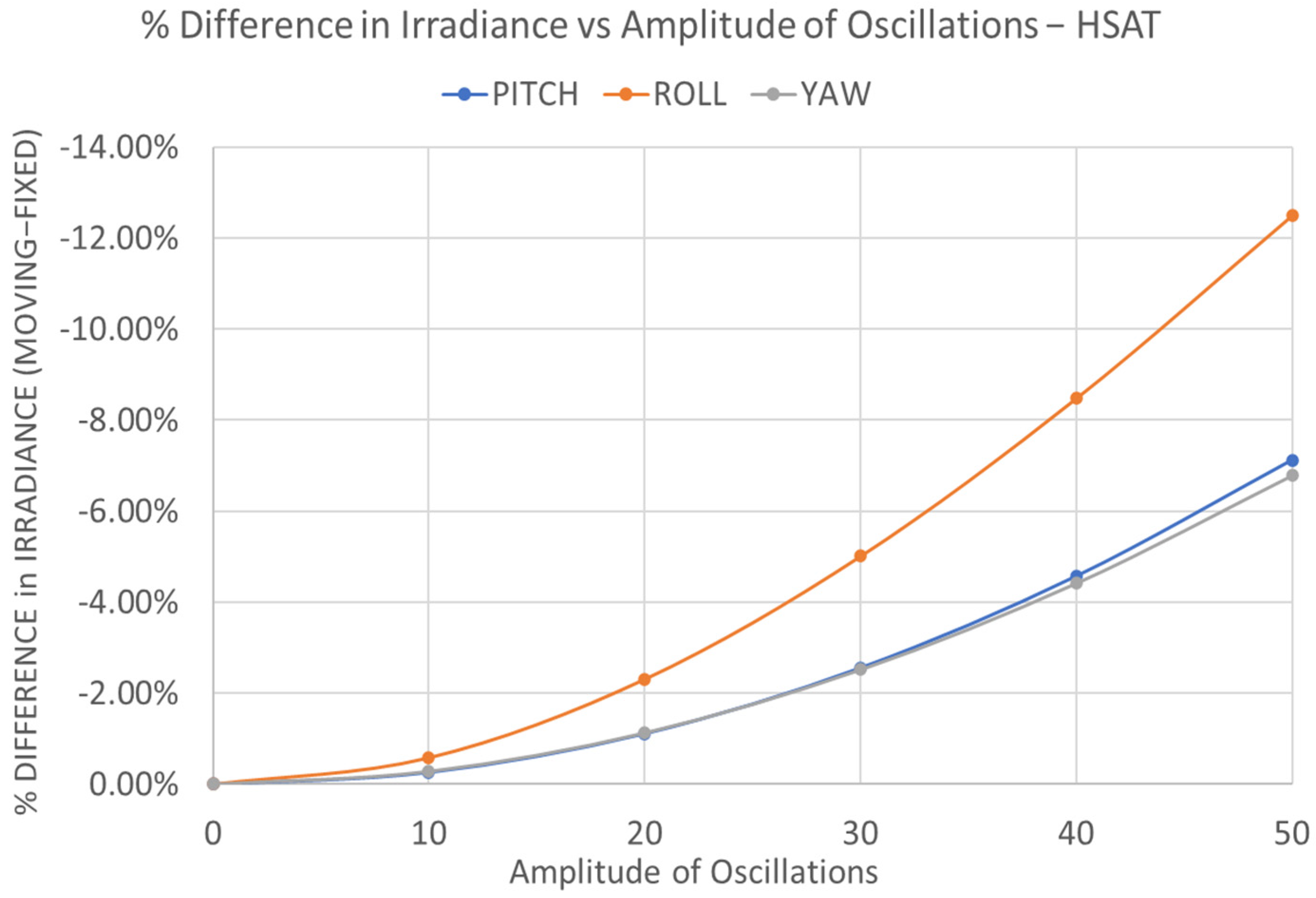
Insolation Deviation of Offshore Tracking Systems from Land—Horizontal Single-Axis Tracking
MonthEffect of PitchEffect of RollEffect of Yaw
January−0.93%−2.31%−1.33%
February−0.96%−2.00%−1.06%
March−0.98%−2.16%−1.14%
April−1.06%−2.06%−0.96%
May−1.15%−2.35%−1.20%
June−1.11%−2.31%−1.13%
July−1.18%−2.38%−1.14%
August−1.10%−2.33%−1.18%
September−1.00%−2.28%−1.24%
October−0.94%−2.20%−1.21%
November−0.98%−2.28%−1.31%
December−0.88%−2.21%−1.34%
Insolation deviation of Offshore Tracking Systems from Land—Vertical Single-Axis Tracking Tilt = 30°
MonthEffect of PitchEffect of RollEffect of Yaw
January−2.07%−1.41%−1.47%
February−1.71%−1.55%−1.07%
March−1.66%−1.83%−1.04%
April−1.53%−1.95%−0.82%
May−1.53%−2.31%−0.95%
June−1.48%−2.28%−0.89%
July−1.54%−2.30%−0.92%
August−1.58%−2.16%−0.99%
September−1.70%−1.93%−1.12%
October−1.83%−1.60%−1.22%
November−2.09%−1.43%−1.46%
December−2.15%−1.30%−1.55%
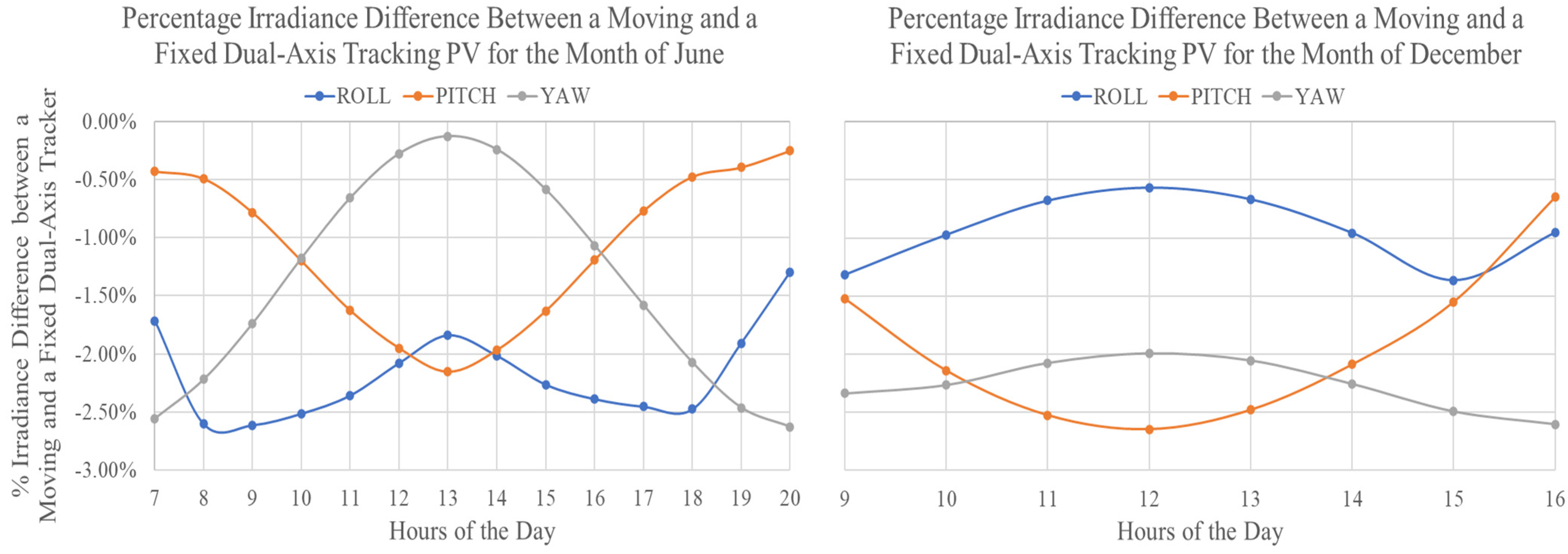
Insolation Deviation of Offshore Tracking Systems from Land —Dual-Axis Tracking
MonthEffect of PitchEffect of RollEffect of Yaw
January−1.95%−1.08%−2.13%
February−1.53%−1.32%−1.60%
March−1.41%−1.75%−1.47%
April−1.30%−1.94%−1.10%
May−1.26%−2.28%−1.26%
June−1.23%−2.25%−1.18%
July−1.29%−2.30%−1.20%
August−1.31%−2.16%−1.32%
September−1.45%−1.83%−1.57%
October−1.65%−1.40%−1.79%
November−1.96%−1.05%−2.12%
December−2.05%−0.90%−2.23%
Table 2. Percentage irradiance difference for a moving and a fixed VSAT PV with different tilts and amplitudes of oscillations for a day in June.
Wave Amplitude = 10°
VSAT TiltEffect of PitchEffect of RollEffect of Yaw
−0.31%−0.39%−0.05%
30°−0.37%−0.57%−0.22%
50°−0.30%−0.57%−0.33%
Wave Amplitude = 20°
−1.49%−1.56%−0.19%
30°−1.48%−2.28%−0.89%
50°−1.18%−2.27%−1.31%
Wave Amplitude = 30°
−3.63%−3.49%−0.42%
30°−3.31%−5.06%−1.99%
50°−2.64%−5.07%−2.93%
Wave Amplitude = 40°
−6.73%−5.99%−0.74%
30°−5.82%−8.78%−3.48%
50°−4.63%−8.88%−5.14%
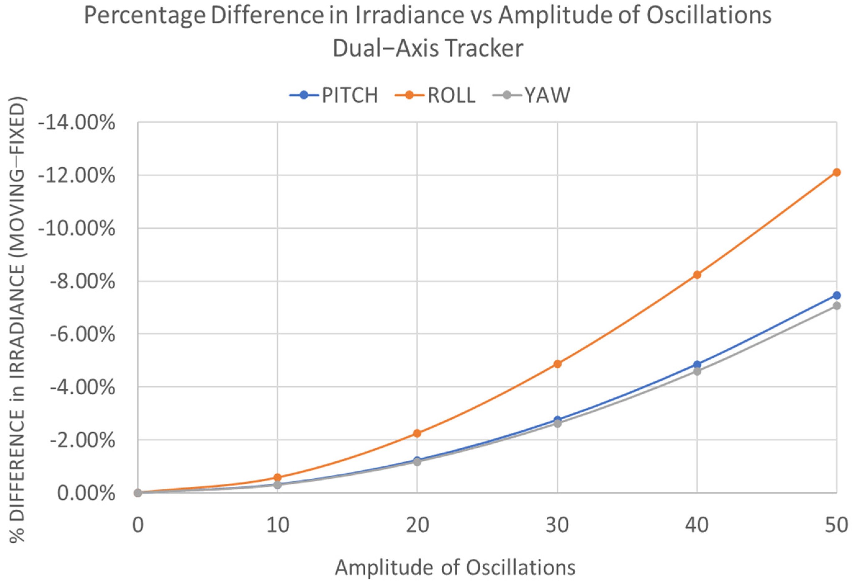
Wave Amplitude = 50°
−10.74%−8.92%−1.14%
30°−8.98%−13.28%−5.35%
50°−6.81%−12.07%−7.89%
Disclaimer/Publisher’s Note: The statements, opinions and data contained in all publications are solely those of the individual author(s) and contributor(s) and not of MDPI and/or the editor(s). MDPI and/or the editor(s) disclaim responsibility for any injury to people or property resulting from any ideas, methods, instructions or products referred to in the content.

