An Improved Q-Axis Current Control to Mitigate the Low-Frequency Oscillation in a Single-Phase Grid-Connected Converter System

Abstract

An electric railway system is a typical single-phase grid-connected converter system, and the low-frequency oscillation (LFO) phenomenon in electric railway systems has been widely reported around the world. Previous research has indicated that the LFO is a small-signal instability issue caused by impedance mismatching between the traction network system and electric trains. Therefore, this paper proposes an improved q-axis current control method to reshape the train’s impedance. The proposed method can be implemented easily by relating a reverse q-axis reactive current directly to the reference of the q-axis current under the dq current decoupled control. Moreover, considering the additional q-axis reactive current control, a small-signal impedance model of a train–network system is built. The impedance-based analysis results indicate that the proposed q-axis reactive current feedback control can increase the magnitude of the train’s impedance, which is beneficial to enhancing the system’s stability. Finally, this paper employs experimental results to verify the effectiveness of the proposed method.

1. Introduction

With the rapid development of electric railway systems, an increasing number of electric trains utilizing flexible converters are being deployed. This has led to improvements in operation speed and carrying capacity. However, due to the interaction between the traction network and the electric train, some instability issues have arisen in train–network system, such as low-frequency oscillation (LFO) [1], harmonic resonance [2], and harmonic instability [3]. Among them, the LFO is particularly prone to occur when multiple trains are simultaneously energized in a rail depot. This can result in low-frequency fluctuations of traction voltage and current, potentially triggering the protection system and delaying normal transportation operations [4].

Currently, since the impedance-based method is simple and effective for analyzing instability problems, it has been widely utilized to assess the LFO in the electric railway system [5,6,7]. Some results have indicated that the LFO is a kind of small-signal instability issue resulting from the impedance mismatching between the traction network and the electric trains [8]. Furthermore, the root cause of the impedance mismatching is then revealed in [9], which clarifies that the negative resistor behavior caused by the DC-link voltage proportional–integrative (PI) controller will lead the LFO under some conditions. Therefore, the core idea of suppressing the LFO is to reshape the impedances of the train and the network for avoiding the impedance mismatching.

On the network side, a passive method by increasing the capacity of the main traction transformer is reported to reduce the impedance of the network [10]. Additionally, some active compensation devices are installed at the network side to mitigate the low-frequency fluctuation of traction voltage. In [11], a single-phase cascaded H-bridge static synchronous compensator (CHB-STATCOM) is proposed to compensate the reactive power in real-time and avoid impedance mismatching between the traction network and electric trains, which is beneficial to mitigate the voltage fluctuation. Although these methods can effectively suppress the LFO, their manufacturing costs are expensive.

Compared with installing additional devices, modifying the controller of the train is an easier and more cost-effective method. At present, nonlinear control and linear control are the two main categories for suppressing the LFO. Some nonlinear control strategies have been proposed to replace the traditional PI controller, such as auto-disturbance rejection control (ADRC) [12], model predictive control (MPC) [13], and interconnection and damping assignment passivity-based control (IDA-PBC) [14]. However, the complexity of the nonlinear control limits their applications. Apart from nonlinear controllers, improved linear controllers have also been researched in depth. With any changes in the linear controller, adaptive tuning of parameters in terms of the operation power is proposed to mitigate the LFO [15]. Additionally, the virtual-impedance-based method is also implemented by feedback or feedforward of voltage and current [16], which gives a clear physical meaning of impedance reshaping. In [9], to reduce the frequency range of negative resistance and increase the impedance magnitude of the train, a proportional–derivative (PD) feedback of the current is applied to provide a positive resistance and reactance. However, the additional loop may affect the dynamic performance of the train in normal steady-state operation. Therefore, some studies utilize a filter to extract the low-frequency oscillatory components, which is used to construct the compensation signal. Since the compensation signal is set as zero under the stable operation model, the impact of an additional loop on the dynamic performance is weakened. In [17], a notch-filter-based active damping control method is proposed. The extracted oscillatory current is feedforward into the current control loop through a damping resistance. Moreover, a power oscillation damper control is also proposed in [18], which utilizes the bandpass filter to extract the oscillatory power for changing the reference signal of the q-axis current dynamically. However, if the oscillatory frequency is close to the fundamental frequency, the oscillatory harmonic component may also be attenuated by filters, which may affect the suppression effects of the LFO.

Therefore, in this paper, an improved q-axis current control is proposed, which cancels the filter and directly relates a reverse q-axis reactive current to the reference of the q-axis current under the dq current decoupled control. The impedance model with consideration of the proposed method is also built to illustrate its impacts on stability. The analysis indicates that the proposed method can prevent impedance mismatching by increasing the impedance magnitude of the electric train.

This paper is then organized as follows: Section 2 concentrates on the proposed control scheme and presents the impedance model with consideration of the improved q-axis current control. In Section 3, the parameter of the proposed method and its impact on stability is investigated. Simulation and experimental verifications are presented in Section 4. Finally, conclusions are drawn in Section 5.

2. Proposed Control Scheme

2.1. System Configuration

The traction network can be considered equivalent to a simple resistor and inductance series circuit in the low-frequency range. Additionally, the electric train can be also simplified as a set of parallel simple two-level rectifiers [10]. As a result, the main circuit of the equivalent and simplified train–network system and its control block diagram are shown in Figure 1.

In Figure 1, the controller of the converter includes a second-order generalized integrator (SOGI), a phase-locked loop (PLL), a current controller (CC), and a DC-link voltage controller (DVC). Here, the current loop is realized in dq-frame with the PI controller. The points of common coupling (PCC) of the voltage space vector and the current space vector are u_s = [u_d u_q]^T and i_s = [i_d i_q]^T, respectively. The main circuit parameters are listed in

Table 1. Parameters of the train–network system.

Parameter	Symbol	Value
AC voltage of the 4 QC	us	1770 V
AC current of the 4 QC	is	7.32 A
Steady-state DC voltage	$u_{\mathrm{dc}}^0$	3600 V
Steady-state d-axis voltage	$u_{\mathrm{d}}^0$	2503 V
Steady-state d-axis current	$i_{\mathrm{d}}^0$	10.4 A
Steady-state q-axis current	$i_{\mathrm{d}}^0$	0 A
Fundamental frequency	f0	50 Hz
Fundamental angle frequency	ω0	314 rad/s
Load resistor of the 4 QC	RL	1000 Ω
Input inductor of the 4 QC	L	10 mH
DC-link capacitor of the 4 QC	Cd	9 mF
SOGI parameters	Ku, Ki	Ku = 0.8, Ki = 0.8
PLL control parameters	Kppll, Kipll	Kppll = 0.012, Kipll = 0.09
CC control parameters	Kpc, Kic	Kpc = 2, Kic = 6
DVC control parameters	Kpv, Kiv	Kpv = 0.6, Kiv = 5
Switch frequency	fsw	500 Hz
Inductance of the network	LS	2 mH

.

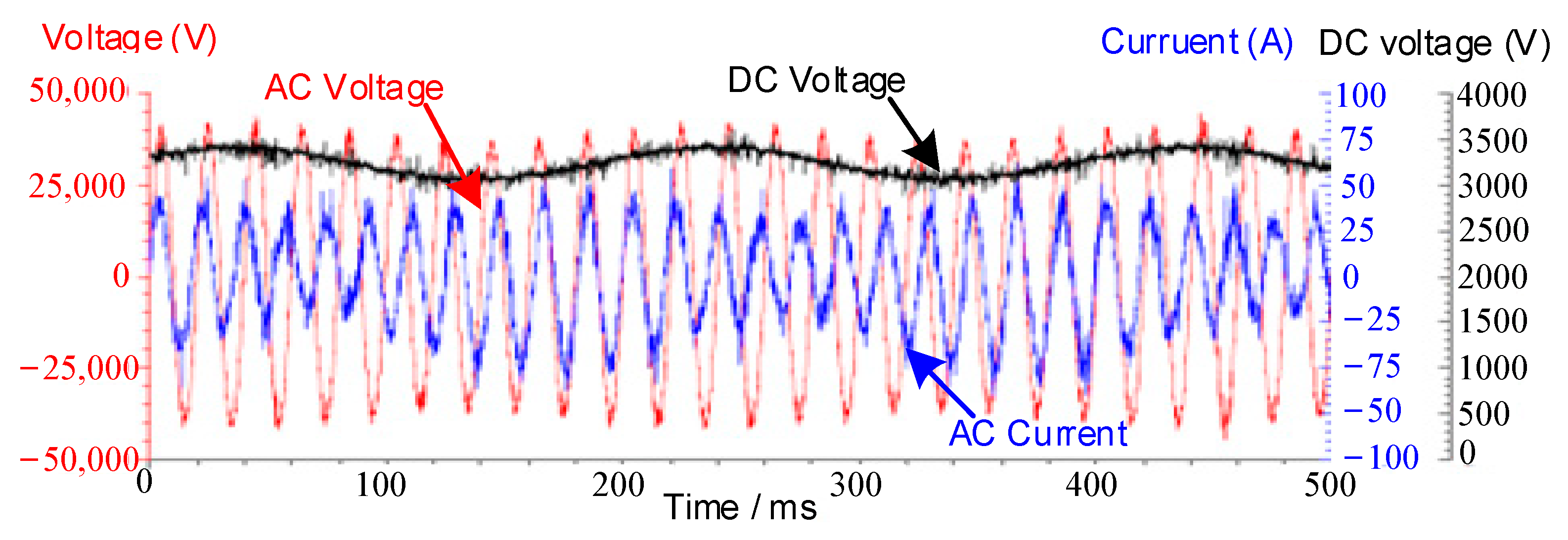
2.2. Field-Measured LFO Waveform

According to the field test result of the LFO in Figure 2, it can be observed that the phase difference between the AC current and the AC voltage is periodic time varying. When the current phase leads the voltage phase, the capacitive reactive power increases the DC-link voltage. In contrast, when the current phase lags in the voltage phase, the inductive reactive power causes a decrease in the DC-link voltage. Therefore, some papers adopt the STATCOM to dynamically compensate the reactive power for mitigating the LFO [11]. However, the cost of the STATCOM is expensive and its controller is complex. It should be mentioned that the advanced electric train is a flexible load that might also be utilized to provide the reactive power to mitigate fluctuation of the voltage.

2.3. Improved Q-Axis Current Control

From Figure 1, it can be observed that the rectifier’s dq decoupled current control involves a reactive current control loop. In a manner similar to STATCOM, a reverse reactive current needs to be incorporated into the reference of the q-axis current to enable dynamic compensation. Therefore, the first step is to extract the oscillatory component to structure the additional signal. The bandpass filter or notch filter are two main methods to obtain the oscillatory component in real time [17,18]. However, when the LFO occurs, in αβ frame, the frequency of the oscillatory component is close to the fundamental frequency [10], which means the narrow bandwidth and fast attenuation performance are necessary to separate two components whose frequencies are close. In addition, the use of a filter can also introduce delay and phase shifts to the extracted oscillation component, which can negatively impact the compensation effect. It is important to note that, in the dq decoupled current control, the q-axis current is calculated in real time and has already been filtered by the sampling filter. When the LFO happens, the q-axis current includes both the DC component and the oscillatory component. Due to the PI control of the q-axis current control loop, the DC component in the q-axis current can track the reference of the q-axis current. Therefore, in the dq frame, the oscillatory component can be easily extracted by removing the DC component of the q-axis current instead of using a filter.

Furthermore, the extracted oscillatory component of the q-axis current should be reversed and added into the reference of the q-axis current, which can inject the reverse reactive current to mitigate the fluctuation of the voltage. Therefore, an improved q-axis current control shown in Figure 3 is then proposed to suppress the LFO.

From Figure 3, when the train operates under the stable condition, the output of the feedback route is zero, which has no impact on tracking the reference of the q-axis current. Additionally, the gain coefficient K is a variable that is used to achieve suppression under different conditions, and its design will be discussed in the following section.

3. Impedance Modeling and Stability Analysis

The proposed method enables real-time injection of a reverse reactive current for mitigating the LFO. The parameter setting is crucial for achieving effective suppression. Therefore, in this section, an impedance model is developed that considers the proposed control approach. This model provides a quantitative analysis that can guide the design of the control parameter.

3.1. Impedance Modeling of the Train in the dq Frame

The dq-impedance model is a classical method to analyze the characteristic of the AC converter. Therefore, the impedance model of the train in the DQ frame is built.

First, for the single-phase system, a virtual β component must be constructed to achieve Park’s transformation by SOGI. The transfer functions of the voltage SOGI and the current SOGI can be expressed as:

$$\left\{\begin{array}{l}{H}_{\alpha \mathrm{u}}(s)=\frac{K_{\mathrm{u}}{\omega }_{0}s}{s^2+K_{\mathrm{u}}{\omega }_{0}s+{\omega }_0^2},H_{\alpha \mathrm{i}}(s)=\frac{K_{\mathrm{i}}{\omega }_{0}s}{s^2+K_{\mathrm{i}}{\omega }_{0}s+{\omega }_0^2}\\ H_{\beta \mathrm{u}}(s)=\frac{K_{\mathrm{u}}{\omega }_0^2}{s^2+K_{\mathrm{u}}{\omega }_{0}s+{\omega }_0^2},H_{\beta \mathrm{i}}(s)=\frac{K_{\mathrm{i}}{\omega }_0^2}{s^2+K_{\mathrm{i}}{\omega }_{0}s+{\omega }_0^2}\end{array}\right.$$

(1)

where ω₀ represents the fundamental angular frequency and s is the Laplace operator.

Due to the dynamic of the PLL, considering the phase perturbation, there are two dq frames: the system dq frame (superscript ‘s’) and the control dq frame (superscript ‘c’). Therefore, considering the impact of PLL and SOGI, the small-signal transfer matrices of voltage and current between the two dq-frames in the frequency domain can be expressed as [10]:

$$\left[\begin{array}{c}\Delta u_{\mathrm{d}}^{\mathrm{c}}\\ \Delta u_q^c\end{array}\right]=G_{\mathrm{upll}}(s)H_{\mathrm{udq}}(s)\left[\begin{array}{c}\Delta u_{\mathrm{d}}^{\mathrm{s}}\\ \Delta u_{\mathrm{q}}^{\mathrm{s}}\end{array}\right]$$

(2)

$$\left[\begin{array}{c}\Delta i_{\mathrm{d}}^{\mathrm{c}}\\ \Delta i_{\mathrm{q}}^{\mathrm{c}}\end{array}\right]=G_{\mathrm{ipll}}(s)H_{\mathrm{udq}}(s)\left[\begin{array}{c}\Delta u_{\mathrm{d}}^{\mathrm{s}}\\ \Delta u_{\mathrm{q}}^{\mathrm{s}}\end{array}\right]+H_{\mathrm{idq}}(s)\left[\begin{array}{c}\Delta i_{\mathrm{d}}^{\mathrm{s}}\\ \Delta i_{\mathrm{q}}^{\mathrm{s}}\end{array}\right]$$

(3)

where

$$\left\{\begin{array}{l}{H}_{\mathrm{udq}}(s)=\frac{1}{2}\left[\begin{array}{cc}{A}_{\mathrm{u}}(s)& B_{\mathrm{u}}(s)\\ -B_{\mathrm{u}}(s)& A_{\mathrm{u}}(s)\end{array}\right],H_{\mathrm{idq}}(s)=\frac{1}{2}\left[\begin{array}{cc}{A}_{\mathrm{i}}(s)& B_{\mathrm{i}}(s)\\ -B_{\mathrm{i}}(s)& A_{\mathrm{i}}(s)\end{array}\right]\\ G_{\mathrm{upll}}(s)=\left[\begin{array}{cc}1& 0\\ 0& 1-u_{\mathrm{d}}^0{G}_{\mathrm{pll}}(s)\end{array}\right],G_{\mathrm{ipll}}(s)=\left[\begin{array}{cc}0& i_{\mathrm{q}}^0{G}_{\mathrm{pll}}(s)\\ 0& -i_{\mathrm{d}}^0{G}_{\mathrm{pll}}(s)\end{array}\right]\\ A_{\mathrm{u}}(s)=\left[\frac{1}{2}{H}_{\alpha \mathrm{u}}(s+j{\omega }_0)+\frac{j}{2}{H}_{\beta \mathrm{u}}(s+j{\omega }_0)\right]+\left[\frac{1}{2}{H}_{\alpha \mathrm{u}}(s-j{\omega }_0)-\frac{j}{2}{H}_{\beta \mathrm{u}}(s-j{\omega }_0)\right]\\ B_{\mathrm{u}}(s)=\left[\frac{j}{2}{H}_{\alpha \mathrm{u}}(s+j{\omega }_0)-\frac{1}{2}{H}_{\beta \mathrm{u}}(s+j{\omega }_0)\right]+\left[\frac{-j}{2}{H}_{\alpha \mathrm{u}}(s-j{\omega }_0)-\frac{1}{2}{H}_{\beta \mathrm{u}}(s-j{\omega }_0)\right]\\ A_{\mathrm{i}}(s)=\left[\frac{1}{2}{H}_{\alpha \mathrm{i}}(s+j{\omega }_0)+\frac{j}{2}{H}_{\beta \mathrm{i}}(s+j{\omega }_0)\right]+\left[\frac{1}{2}{H}_{\alpha \mathrm{i}}(s-j{\omega }_0)-\frac{j}{2}{H}_{\beta \mathrm{i}}(s-j{\omega }_0)\right]\\ B_{\mathrm{i}}(s)=\left[\frac{j}{2}{H}_{\alpha \mathrm{i}}(s+j{\omega }_0)-\frac{1}{2}{H}_{\beta \mathrm{i}}(s+j{\omega }_0)\right]+\left[\frac{-j}{2}{H}_{\alpha \mathrm{i}}(s-j{\omega }_0)-\frac{1}{2}{H}_{\beta \mathrm{i}}(s-j{\omega }_0)\right]\\ G_{\mathrm{pll}}(s)=\frac{K_{\mathrm{ppll}}+K_{\mathrm{ipll}}/s}{s+u_{\mathrm{d}}^0\left(K_{\mathrm{ppll}}+K_{\mathrm{ipll}}/s\right)}\end{array}\right.$$

In Equation (3), the superscript ‘0′ represents the steady-state values of the voltages and currents. The symbol Δ represents the perturbation components.

As shown in Figure 1, the DC-link voltage controller provides the reference of the d-axis current, which can be expressed under the system dq frame as:

$$\Delta i_{\mathrm{dref}}=\left[\begin{array}{cc}-H_{\mathrm{v}}(s)G_1(s)& -H_{\mathrm{v}}(s)G_2(s)\end{array}\right]\left[\begin{array}{c}\Delta i_{\mathrm{d}}^{\mathrm{s}}\\ \Delta i_{\mathrm{q}}^{\mathrm{s}}\end{array}\right]+\left[\begin{array}{cc}-H_{\mathrm{v}}(s)G_3(s)& -H_{\mathrm{v}}(s)G_4(s)\end{array}\right]\left[\begin{array}{c}\Delta u_{\mathrm{d}}^{\mathrm{s}}\\ \Delta u_{\mathrm{q}}^{\mathrm{s}}\end{array}\right]$$

(4)

where

$$\left\{\begin{array}{l}{G}_1(s)=\frac{0.5u_{\mathrm{d}}^0}{s{C}_{\mathrm{d}}{u}_{\mathrm{dc}}^0+u_{\mathrm{dc}}^0/R_{\mathrm{L}}},G_2(s)=\frac{0.5u_{\mathrm{q}}^0}{s{C}_{\mathrm{d}}{u}_{\mathrm{dc}}^0+u_{\mathrm{dc}}^0/R_{\mathrm{L}}}\\ G_3(s)=\frac{0.5i_{\mathrm{d}}^0}{s{C}_{\mathrm{d}}{u}_{\mathrm{dc}}^0+u_{\mathrm{dc}}^0/R_{\mathrm{L}}},G_4(s)=\frac{0.5i_{\mathrm{q}}^0}{s{C}_{\mathrm{d}}{u}_{\mathrm{dc}}^0+u_{\mathrm{dc}}^0/R_{\mathrm{L}}}\\ H_{\mathrm{v}}(s)=K_{\mathrm{pv}}+\frac{K_{\mathrm{iv}}}{s}\end{array}\right.$$

Since the reference of the q-axis current is restructured by the improved q-axis current control, its small-signal model in the system dq frame is derived as:

$$\Delta i_{\mathrm{qref}}=\frac{i_{\mathrm{d}}^{0}K{G}_{\mathrm{pll}}(s)}{2}\left[\begin{array}{cc}-B_{\mathrm{u}}(s)& A_{\mathrm{u}}\end{array}(s)\right]\left[\begin{array}{c}\Delta u_{\mathrm{d}}^{\mathrm{s}}\\ \Delta u_{\mathrm{q}}^{\mathrm{s}}\end{array}\right]-\frac{K}{2}\left[\begin{array}{cc}-B_{\mathrm{i}}(s)& A_{\mathrm{i}}\end{array}(s)\right]\left[\begin{array}{c}\Delta i_{\mathrm{d}}^{\mathrm{s}}\\ \Delta i_{\mathrm{q}}^{\mathrm{s}}\end{array}\right]$$

(5)

According to (4) and (5), the small-signal model of the current references under the system dq frame are expressed as:

$$\left[\begin{array}{c}\Delta {\mathrm{i}}_{\mathrm{dref}}\\ \Delta {\mathrm{i}}_{\mathrm{qref}}\end{array}\right]=\underset{G_{\mathrm{i}}(s)}{\underbrace{\left[\begin{array}{cc}-H_{\mathrm{v}}(s)G_1(s)& -H_{\mathrm{v}}(s)G_2(s)\\ \frac{K{B}_{\mathrm{i}}(s)}{2}& -\frac{K{A}_{\mathrm{i}}(s)}{2}\end{array}\right]}}\left[\begin{array}{c}\Delta i_{\mathrm{d}}^{\mathrm{s}}\\ \Delta i_{\mathrm{q}}^{\mathrm{s}}\end{array}\right]+\underset{G_{\mathrm{v}}(s)}{\underbrace{\left[\begin{array}{cc}-H_{\mathrm{v}}(s)G_3(s)& -H_{\mathrm{v}}{G}_4(s)(s)\\ \frac{i_{\mathrm{d}}^{0}K{B}_{\mathrm{u}}(s)G_{\mathrm{pll}}(s)}{2}& -\frac{i_{\mathrm{d}}^{0}K{A}_{\mathrm{u}}(s)G_{\mathrm{pll}}(s)}{2}\end{array}\right]}}\left[\begin{array}{c}\Delta u_{\mathrm{d}}^{\mathrm{s}}\\ \Delta u_{\mathrm{q}}^{\mathrm{s}}\end{array}\right]$$

(6)

The current loop provides the reference of the modulation voltage, which can be expressed under the control dq frame as:

$$\left[\begin{array}{c}\Delta u_{\mathrm{abdref}}^{\mathrm{c}}\\ \Delta u_{\mathrm{abqref}}^{\mathrm{c}}\end{array}\right]=\left[\begin{array}{c}\Delta u_{\mathrm{d}}^{\mathrm{c}}\\ \Delta u_{\mathrm{q}}^{\mathrm{c}}\end{array}\right]-{\mathbf{H}}_{\mathrm{i}}(s)\left[\begin{array}{c}\Delta i_{\mathrm{dref}}^{}-\Delta i_{\mathrm{d}}^{\mathrm{c}}\\ \Delta i_{\mathrm{qref}}^{}-\Delta i_{\mathrm{q}}^{\mathrm{c}}\end{array}\right]+\underset{G_{\omega \mathrm{L}}}{\underbrace{\left[\begin{array}{cc}0& {\omega }_{0}L\\ -{\omega }_{0}L& 0\end{array}\right]}}\left[\begin{array}{c}\Delta i_{\mathrm{d}}^{\mathrm{c}}\\ \Delta i_{\mathrm{q}}^{\mathrm{c}}\end{array}\right]$$

(7)

where $H_{\mathrm{i}}(s)=\left[\begin{array}{cc}{K}_{\mathrm{pc}}+\frac{K_{\mathrm{ic}}}{s}& 0\\ 0& K_{\mathrm{pc}}+\frac{K_{\mathrm{ic}}}{s}\end{array}\right]$.

According to circuit relationships, in the system dq frame, the actual modulation voltage can be expressed as:

$$\left[\begin{array}{c}\Delta u_{\mathrm{abd}}^{\mathrm{s}}\\ \Delta u_{\mathrm{abq}}^{\mathrm{s}}\end{array}\right]=\left[\begin{array}{c}\Delta u_{\mathrm{d}}^{\mathrm{s}}\\ \Delta u_{\mathrm{q}}^{\mathrm{s}}\end{array}\right]-\underset{G_{\mathrm{rl}}(s)}{\underbrace{\left[\begin{array}{cc}R+sL& -{\omega }_{0}L\\ {\omega }_{0}L& R+sL\end{array}\right]}}\left[\begin{array}{c}\Delta i_{\mathrm{d}}^{\mathrm{s}}\\ \Delta i_{\mathrm{q}}^{\mathrm{s}}\end{array}\right]$$

(8)

Due to the delay in the digital control and PWM [20], the relationship between the reference of the modulation voltage and the actual modulation voltage is expressed as:

$$\left[\begin{array}{c}\Delta u_{\mathrm{abd}}^{\mathrm{s}}\\ \Delta u_{\mathrm{abq}}^{\mathrm{s}}\end{array}\right]=G_{\mathrm{d}}(s)\left[\begin{array}{c}\Delta u_{\mathrm{abdref}}^{\mathrm{s}}\\ \Delta u_{\mathrm{abqref}}^{\mathrm{s}}\end{array}\right]$$

(9)

where $G_{\mathrm{d}}(s)=e^{-T_{\mathrm{d}}s}$, and T_d is the delay time of the PWM.

According to Equations (1)–(9), the impedance model of the train in the system dq frame can be expressed as:

$$Z_{t,dq}^{re}(s)={\left[I-G_{\mathrm{d}}\left(H_{\mathrm{i}}{G}_{\mathrm{ipll}}{H}_{\mathrm{udq}}-H_{\mathrm{i}}{G}_{\mathrm{v}}+H_{\mathrm{udq}}\right)\right]}^{-1}\cdot \left[G_{\mathrm{rl}}-G_{\mathrm{d}}{H}_{\mathrm{i}}{G}_{\mathrm{i}}+G_{\mathrm{d}}(H_{\mathrm{i}}+G_{\omega \mathrm{L}})H_{\mathrm{idq}}\right]$$

(10)

3.2. Impact of the Proposed Control Scheme on the Impedance

The proposed q-axis current control has a controlled gain coefficient, K. To illustrate its impact on the impedance, three different values are selected. The impedance curves in the dq frame under different gain coefficients are shown in Figure 4.

In Figure 4, it is evident that increasing the gain coefficient mainly increases the magnitudes of the q-q channel impedance and the d-q channel impedance in the low-frequency range. It has a slight impact on the d-d channel impedance and q-q channel impedance. In [9], it was shown that increasing the impedance’s magnitude is beneficial to stability. Therefore, the proposed method may improve the stability of the train–network system. As observed, the increased impedance magnitude is related to the gain coefficient, K. Thus, designing the K is crucial for mitigating the LFO.

3.3. Design of the Gain Coefficient Based on SISO Equivalent Model

3.3.1. SISO Equivalent Model of the Train–Network System

The previous impedance model in (9) is built under the real-vector dq frame [21]. As noticed, the impedance matrixes of the train–network system are two-order matrixes and both are non-diagonal matrixes. For this multiple-input and multiple-output (MIMO) system, the generalized Nyquist criterion is used to judge the stability, which is inconvenient to design the gain coefficient. Therefore, a single-input and single-output (SISO) equivalent method of the MIMO system is proposed under the complex-vector dq frame to simplify this analysis. The equivalent SISO system has the same closed-loop transfer function as the original MIMO system [22,23,24]. Therefore, the stability of the MIMO system can be judged by the equivalent SISO system.

The impedance matrix under the real-vector dq frame can be transferred to the complex-vector dq frame by using a linear transformation [23]. Then, the impedance matrixes of the train and network in the complex-vector dq frame are expressed as:

$$Z_{g,dq}^{com}(s)=A_Z^{}\left[\begin{array}{cc}{R}_s+s{L}_s& -{\omega }_0{L}_s\\ {\omega }_0{L}_s& R_s+s{L}_s\end{array}\right]A_Z^{-1}=\left[\begin{array}{cc}{Z}_{g,+}(s)& \\ & Z_{g,+}^{*}(s)\end{array}\right]$$

(11)

$$Z_{t,dq}^{com}(s)=A_Z^{}{Z}_{t.dq}^{re}(s)A_Z^{-1}=\left[\begin{array}{cc}{Z}_{t,+}(s)& Z_{t,-}(s)\\ Z_{t,-}^{*}(s)& Z_{g,+}^{*}(s)\end{array}\right]$$

(12)

where $A_{\mathrm{Z}}=\frac{1}{\sqrt{2}}\left[\begin{array}{cc}1& j\\ 1& -j\end{array}\right],A_{\mathrm{Z}}^{-1}=A_{\mathrm{Z}}^{*}=\frac{1}{\sqrt{2}}\left[\begin{array}{cc}1& 1\\ -j& j\end{array}\right]$.

Since the impedance of the network is symmetrical in the dq frame, its impedance matrix in the complex-vector dq frame is a diagonal matrix. However, due to asymmetrical control loops, such as PLL and DVC, the impedance matrix of the train is an off-diagonal matrix. According to the SISO equivalent technology in [22], the SISO equivalent impedance of the network is expressed as:

$$Z_g^{siso}(s)=Z_{g,+}(s)=R_s+(s+j{\omega }_0)L_s$$

(13)

Considering the non-diagonal elements in (12), the SISO equivalent impedance of the train is expressed as:

$$Z_t^{siso}(s)=Z_{t,+}(s)-\frac{Z_{t,-}(s)Z_{t,-}^{*}(s)}{Z_{g,+}^{*}(s)+Z_{t,+}^{*}(s)}$$

(14)

Using the SISO equivalent model of the train–network system, the stability can be assessed by applying the Nyquist criterion, which aligns with Equation (15). This approach simplifies the stability analysis and facilitates the design of the gain coefficient.

$$T(s)=\frac{Z_g^{siso}(s)}{Z_t^{siso}(s)}=\frac{\left|Z_g^{siso}(s)\right|}{\left|Z_t^{siso}(s)\right|}\left[\angle Z_g^{siso}(s)-\angle Z_t^{siso}(s)\right]$$

(15)

As shown in Equation (15), the train–network system is stable if the phase difference at the magnitude interactive frequency is less than 180°. To clarify the influence of the train quantity on stability, SISO equivalent impedance curves are plotted in Figure 5.

From Figure 5, it can be observed that the impedance of the train exhibits negative resistance in the low-frequency range. When only one train is energized, there is no magnitude intersection in this frequency range, indicating that the train–network is stable. However, as the number of energized trains increases to five, the magnitude of the equivalent train impedance decreases. Consequently, the frequency of the magnitude intersection shifts into the negative resistance range, causing the phase difference to exceed 180°, resulting in instability.

3.3.2. Design Principle of the Gain Coefficient

According to the previous analysis results, if there is no magnitude intersection in the negative resistance range, the system is stable. Therefore, increasing the magnitude of the train is a feasible approach to mitigate the LFO. In terms of the impact of the improved q-axis current control on the train’s impedance in Figure 4, the gain coefficient K has significant impact on the magnitude of the train’s impedance. Therefore, the basic design principle is that the K should reshape the impedance to guarantee no magnitude intersection in the negative resistor range.

Typically, the frequency range of the LFO is around 1–10 Hz [10]. Let s = jω, to prevent the LFO; then, the minimum magnitude value of the train impedance in this frequency range should be greater than the magnitude of the network impedance. This condition is consistent with Equation (16).

$$\min \left\{\left|Z_t^{siso}(j2\pi f,K)\right|-\left|Z_g^{siso}(j2\pi f)\right|\right\}>0,f\in \left[\begin{array}{cc}1\mathrm{Hz}& 10\mathrm{Hz}\end{array}\right]$$

(16)

It should be noted that the condition in Equation (16) is conservative, meaning that a stable system may not necessarily satisfy it. When the number of energized trains is set to 5, the effect of different gain coefficients on the magnitude can be visualized using Equation (16) over the frequency range of 1–10 Hz. The responses are plotted in a 3D coordinate system in Figure 6. As observed from the figure, the condition in Equation (16) is satisfied in the entire low-frequency range when the gain coefficient is greater than 10. Furthermore, a conservative boundary for the gain coefficient K of a stable system is plotted in Figure 7 for different inductances of the network. In Figure 7, it is shown that increasing gain K can mitigate the LFO under the weaker network.

3.4. Stability Improvement

According to Figure 7, it can be seen that the gain K should be larger than 10 under L_s = 2 mH and n = 5. Therefore, in this case, the gain K is set as 12. The effect of K on reshaping the SISO equivalent impedance model of the train is clearly shown in Figure 8.

In Figure 8, it can be observed that the addition of the feedback route in the q-axis current control leads to an increase in the magnitude of the train’s impedance. This shift in impedance results in the magnitude intersection moving out of the negative resistor range, thereby improving the stability of the train–network system and providing a positive phase margin of approximately 17.6°. A time-domain simulation result using Simulink is presented in Figure 9.

In Figure 9, when 5 trains energize under the same rail depot, the LFO is induced, and its oscillatory frequency is about 6 Hz. The enlarged waveforms from 1.2 s to 1.6 s show that the phase difference between the voltage and the current is periodic and time varying, which is consistent with the field-measured results. Furthermore, after 2 s, the improved q-axis current control is applied, and the time-domain simulation result indicates that the LFO is effectively suppressed when the gain coefficient K is set to 12.

3.5. Impact of the Proposed Method on the Dynamic Performance

The improved q-axis current control changes the structure of the original reactive current control. Hence, the impact of the proposed method on the dynamic performance of the train is discussed in this part.

The proposed method adds an additional signal to the reference of the q-axis current. In the steady-state operation mode, when the reference of the q-axis current is suddenly changed, the improved q-axis current control should also track the new reference signal. Therefore, three reference values of the q-axis current are set. The time-domain simulation results of the q-axis current are shown in Figure 10.

From Figure 10, it can be seen that the improved q-axis current control can effectively track different references of the q-axis current. In addition, it also reduces the fluctuation of the current.

Moreover, the sudden change in load is frequent when the train operates under the normal condition. Therefore, the impact of the proposed method on the dc-link voltage is also studied under the condition of a sudden change in load. The time-domain waveforms are shown in Figure 11.

In Figure 11, it can be observed that the dynamic responses of the DC-link voltage are similar when using the original q-axis current control and the improved q-axis current control. Therefore, it can be concluded that the improved q-axis current control does not have a significant impact on the dynamic performance of the DC-link voltage under normal operating conditions.

4. Verification

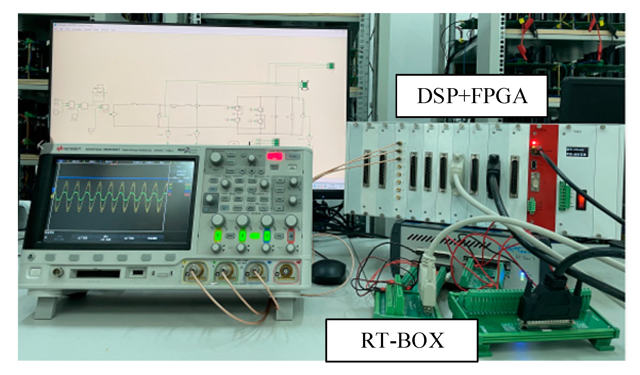
4.1. Experimental Setup

In order to validate the theoretical analysis in previous sections, a hardware-in-the-loop (HIL) platform of the simplified train–network system shown in Figure 12 was built. The hardware of the single-phase rectifier was built in the power electronics simulation software PLECS and runs on a real-time simulator RT-BOX with a time step of 2 μs. The control algorithm was implemented in the TMS320C28346 digital signal processing controller (DSP), and the sampling frequency was set as 10 kHz. The Xilinx XC6SLX16 field programmable gate array (FPGA) was adopted to achieve the modulation scheme. Additionally, a host computer was used to modify the control parameters in real time. The voltage and current waveforms were captured by an oscilloscope. The parameters of the HIL tests are listed in Table 1.

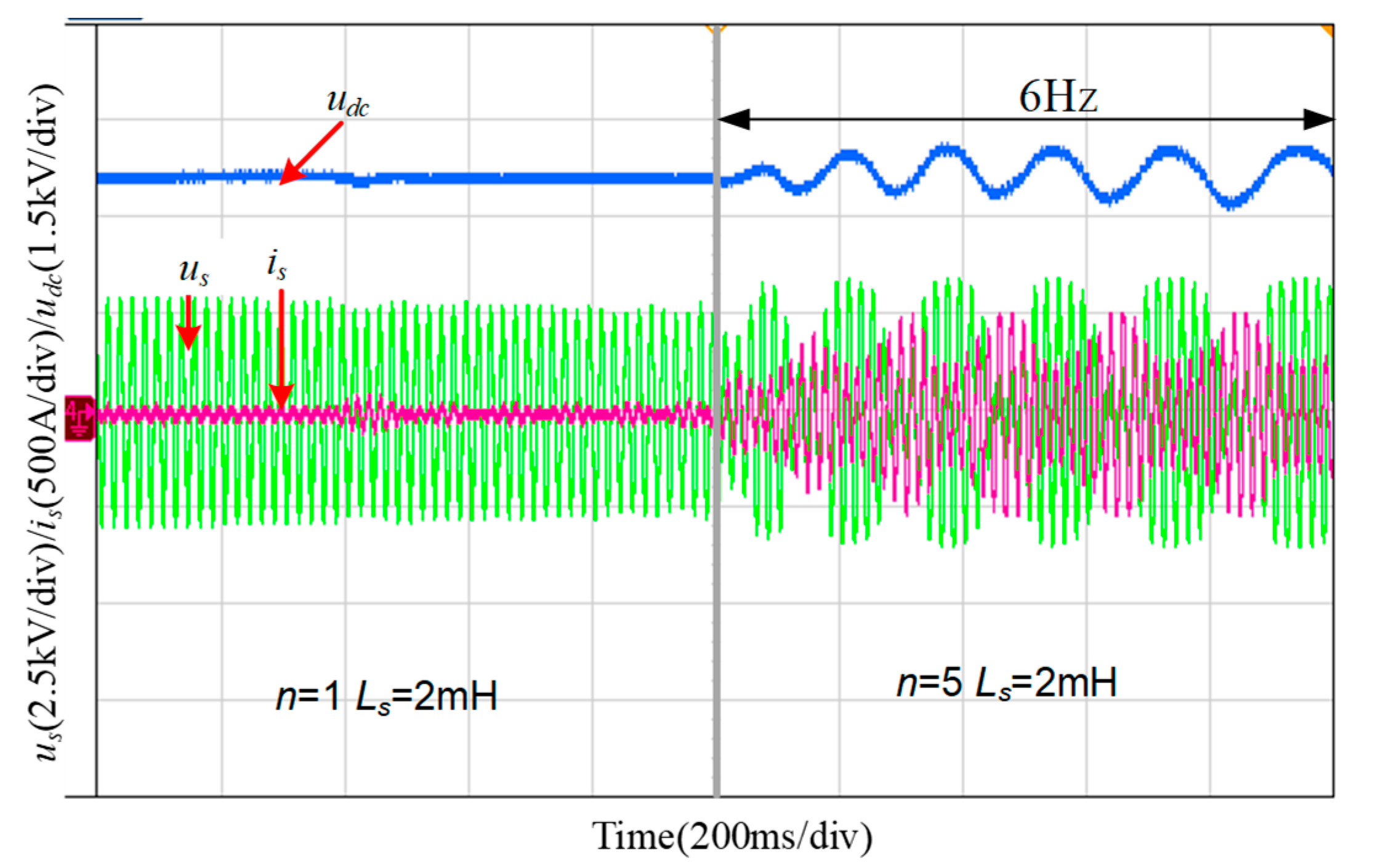
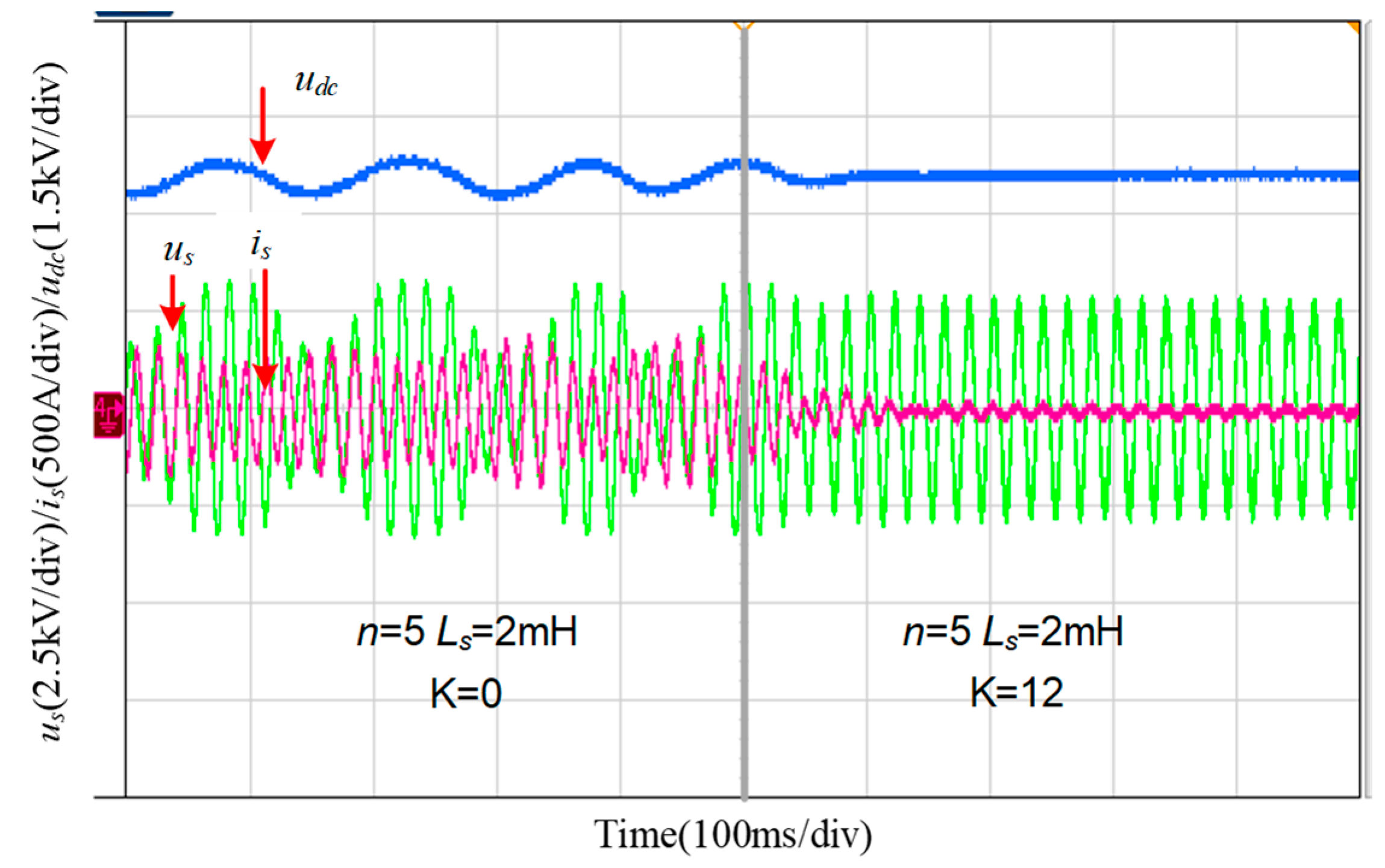
4.2. Experimental Results

The HIL test results under different numbers of energized trains are shown in Figure 13. In this case, the equivalent inductance of the traction network is set as 2 mH. When one train is connected to the traction network, the train–network system is stable. However, it can be found that a 6 Hz oscillation occurs when the number of energized trains is increased from 1 to 5. The experimental stability results and oscillatory frequency are the same as the theoretical stability predictions shown in Figure 5.

The HIL test results under different q-axis current controllers are shown in Figure 14. In Figure 14, it can be found that the LFO is suppressed when K is increased from 0 to 12. Therefore, the proposed improved q-axis current control can enhance the small-signal stability of the train–network system and avoid the LFO. The experimental stability result is also same as the theoretical stability predictions shown in Figure 8.

5. Conclusions

In this paper, an improved q-axis current control for trains in the train–network system is proposed to suppress the LFO. This method involves relating a reverse q-axis reactive current to the reference of the q-axis current under the dq current decoupled control. Based on the study, some valuable conclusions can be drawn:

(1)

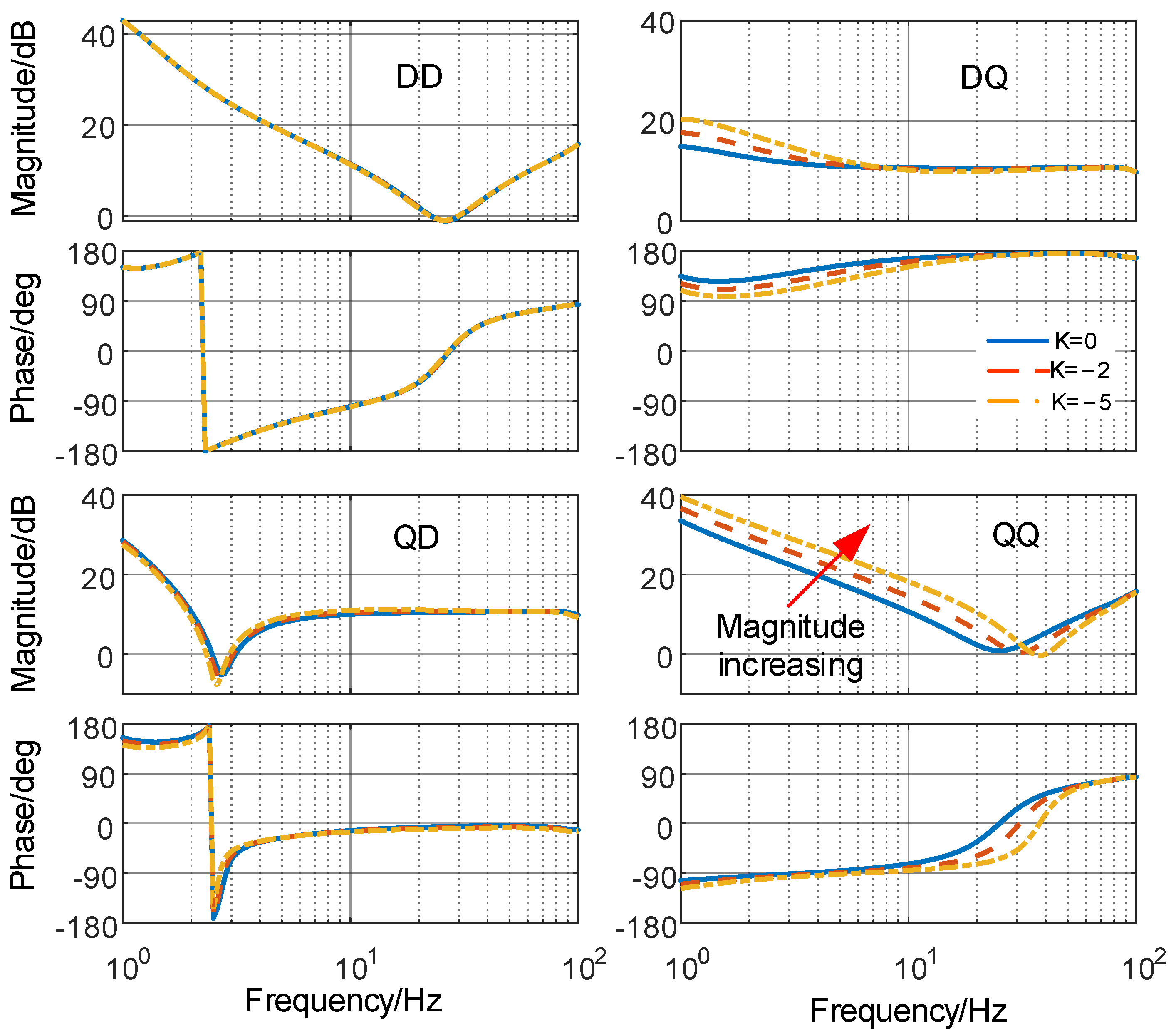
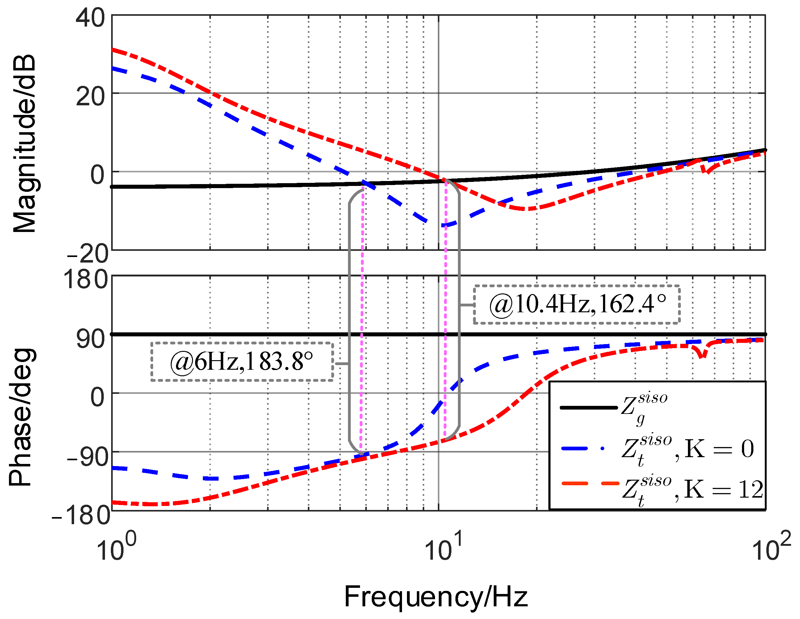
The proposed q-axis current control increases the magnitude of the input impedance of the train. A higher gain coefficient K in the proposed method can provide a higher impedance magnitude. Based on the impedance ratio criterion, the improved q-axis current control reduces the modulus of the ratio between the impedance of the traction network and the impedance of the train, which is beneficial for the small-signal stability of the train–network system.

(2)

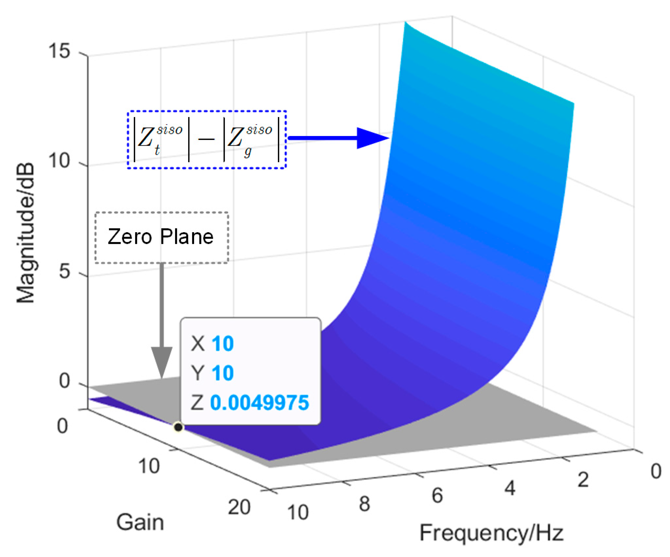
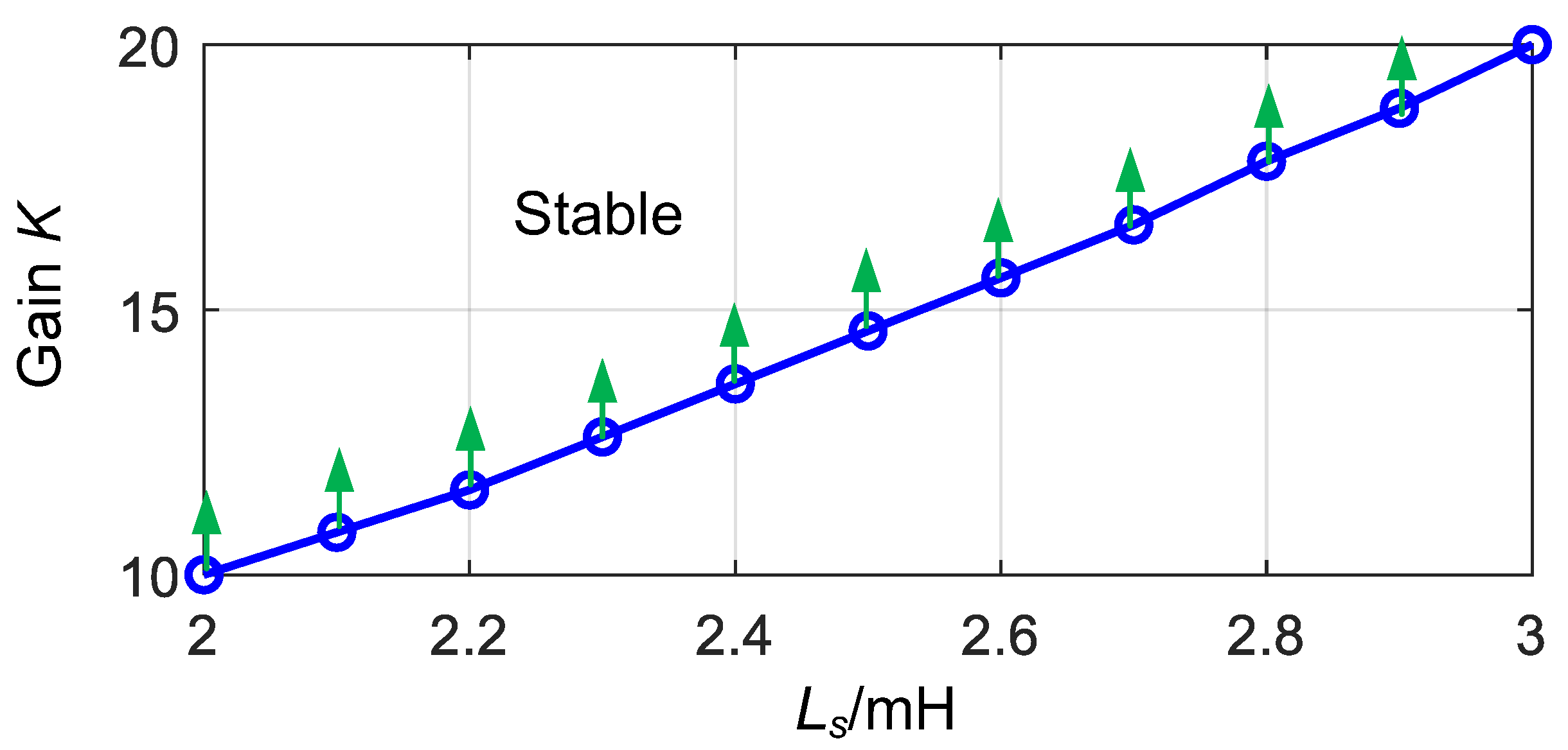
A design approach for quantizing the gain coefficient K is proposed based on the SISO equivalent impedance model. The fundamental design principle is that the minimum value of K should ensure that there is no intersection of impedance magnitude between the traction network and the train in the negative resistor range.

(3)

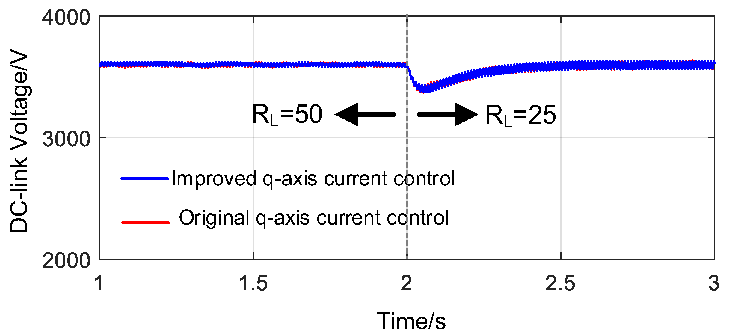
The improved q-axis current control has no effects on the dynamic performance of the DC-link voltage under the normal operation mode.

References

1. Hu, H.; Tao, H.; Blaabjerg, F.; Wang, X.; He, Z.; Gao, S. Train–Network Interactions and Stability Evaluation in High-Speed Railways–Part I: Phenomena and Modeling. IEEE Trans. Power Electron. 2017, 33, 4627–4642. [Google Scholar] [CrossRef]
2. Hu, H.; Shao, Y.; Tang, L.; Ma, J.; He, Z.; Gao, S. Overview of Harmonic and Resonance in Railway Electrification Systems. IEEE Trans. Ind. Appl. 2018, 54, 5227–5245. [Google Scholar] [CrossRef]
3. Tao, H.; Hu, H.; Wang, X.; Blaabjerg, F.; He, Z. Impedance-Based Harmonic Instability Assessment in a Multiple Electric Trains and Traction Network Interaction System. IEEE Trans. Ind. Appl. 2018, 54, 5083–5096. [Google Scholar] [CrossRef]
4. Wang, H.; Mingli, W.; Sun, J. Analysis of Low-Frequency Oscillation in Electric Railways Based on Small-Signal Modeling of Vehicle-Grid System in dq Frame. IEEE Trans. Power Electron. 2015, 30, 5318–5330. [Google Scholar] [CrossRef]
5. Liao, Y.; Liu, Z.; Zhang, H.; Wen, B. Low-Frequency Stability Analysis of Single-Phase System with dq-Frame Impedance Approach—Part I: Impedance Modeling and Verification. IEEE Trans. Ind. Appl. 2018, 54, 4999–5011. [Google Scholar] [CrossRef]
6. Jiang, X.; Hu, H.; He, Z.; Tao, H.; Qian, Q. Study on low-frequency voltage fluctuation of traction power supply system introduced by multiple modern trains. Electr. Power Syst. Res. 2017, 146, 246–257. [Google Scholar] [CrossRef]
7. Jiang, K.; Zhang, C.; Ge, X. Low-Frequency Oscillation Analysis of the Train-Grid System Based on an Improved Forbidden-Region Criterion. IEEE Trans. Ind. Appl. 2018, 54, 5064–5073. [Google Scholar] [CrossRef]
8. Liao, Y.; Liu, Z.; Zhang, H.; Wen, B. Low-Frequency Stability Analysis of Single-Phase System With dq-Frame Impedance Approach—Part II: Stability and Frequency Analysis. IEEE Trans. Ind. Appl. 2018, 54, 5012–5024. [Google Scholar] [CrossRef]
9. Zhou, Y.; Hu, H.; Yang, X.; Yang, J.; He, Z.; Gao, S. Low Frequency Oscillation Traceability and Suppression in Railway Electrification Systems. IEEE Trans. Ind. Appl. 2019, 55, 7699–7711. [Google Scholar] [CrossRef]
10. Hu, H.; Zhou, Y.; Li, X.; Lei, K. Low-Frequency Oscillation in Electric Railway Depot: A Comprehensive Review. IEEE Trans. Power Electron. 2020, 36, 295–314. [Google Scholar] [CrossRef]
11. Wu, S.; Liu, Z.; Li, Z.; Zhang, H.; Hu, X. Impedance Modeling and Stability Analysis in Vehicle-Grid System with CHB-STATCOM. IEEE Trans. Power Syst. 2020, 35, 3026–3039. [Google Scholar] [CrossRef]
12. Zhang, G.; Liu, Z.; Yao, S.; Liao, Y.; Xiang, C. Suppression of Low-Frequency Oscillation in Traction Network of High-Speed Railway Based on Auto-Disturbance Rejection Control. IEEE Trans. Transp. Electrif. 2016, 2, 244–255. [Google Scholar] [CrossRef]
13. Liu, Z.; Wang, Y.; Liu, S.; Li, Z.; Zhang, H.; Zhang, Z. An Approach to Suppress Low-Frequency Oscillation by Combining Extended State Observer With Model Predictive Control of EMUs Rectifier. IEEE Trans. Power Electron. 2019, 34, 10282–10297. [Google Scholar] [CrossRef]
14. Liu, Z.; Geng, Z.; Hu, X. An Approach to Suppress Low Frequency Oscillation in the Traction Network of High-Speed Railway Using Passivity-Based Control. IEEE Trans. Power Syst. 2018, 33, 3909–3918. [Google Scholar] [CrossRef]
15. Jiang, X.; Hu, H.; Yang, X.; He, Z.; Qian, Q.; Tricoli, P. Analysis and Adaptive Mitigation Scheme of Low-Frequency Oscillations in AC Railway Traction Power Systems. IEEE Trans. Transp. Electrif. 2019, 5, 715–726. [Google Scholar] [CrossRef]
16. Wang, X.; Li, Y.W.; Blaabjerg, F.; Loh, P.C. Virtual-Impedance-Based Control for Voltage-Source and Current-Source Converters. IEEE Trans. Power Electron. 2014, 30, 7019–7037. [Google Scholar] [CrossRef]
17. Shuai, Z.; Cheng, H.; Xu, J.; Shen, C.; Hong, Y.; Li, Y. A Notch Filter-Based Active Damping Control Method for Low-Frequency Oscillation Suppression in Train–Network Interaction Systems. IEEE J. Emerg. Sel. Top. Power Electron. 2019, 7, 2417–2427. [Google Scholar] [CrossRef]
18. Danielsen, S. Electric Traction Power System Stability. Ph.D. Thesis, Norwegian University of Science and Technology, Trondheim, Norway, 2010. [Google Scholar]
19. Li, J.; Wu, M. Measurement and Analysis on Low-Frequency Oscillation in Xuzhou Electrical Railway Hub. In Proceedings of the 2015 International Conference on Electrical and Information Technologies for Rail Transportation, Zhuzhou, China, 17–19 October 2015; pp. 659–666. [Google Scholar]
20. Wen, B.; Boroyevich, D.; Burgos, R.; Mattavelli, P.; Shen, Z. Analysis of D-Q Small-Signal Impedance of Grid-Tied Inverters. IEEE Trans. Power Electron. 2015, 31, 675–687. [Google Scholar] [CrossRef]
21. Harnefors, L. Modeling of Three-Phase Dynamic Systems Using Complex Transfer Functions and Transfer Matrices. IEEE Trans. Ind. Electron. 2007, 54, 2239–2248. [Google Scholar] [CrossRef]
22. Zhang, C.; Cai, X.; Rygg, A.; Molinas, M. Sequence Domain SISO Equivalent Models of a Grid-Tied Voltage Source Converter System for Small-Signal Stability Analysis. IEEE Trans. Energy Convers. 2017, 33, 741–749. [Google Scholar] [CrossRef]
23. Rygg, A.; Molinas, M.; Zhang, C.; Cai, X. A Modified Sequence-Domain Impedance Definition and Its Equivalence to the dq-Domain Impedance Definition for the Stability Analysis of AC Power Electronic Systems. IEEE J. Emerg. Sel. Top. Power Electron. 2016, 4, 1383–1396. [Google Scholar] [CrossRef]
24. Liao, K.; Pang, B.; Yang, J.; He, Z. Compensation Strategy of Wideband Voltage Harmonics for Doubly-Fed Induction Generator. IEEE Trans. Energy Convers. 2022, 38, 674–684. [Google Scholar] [CrossRef]
Figure 1. Block diagram of the simplified single-phase train–network system.
Energies 16 03816 g001
Figure 2. Field-measured waveforms of the LFO [19].
Energies 16 03816 g002
Figure 3. Improved q-axis current control scheme.
Energies 16 03816 g003
Figure 4. Impacts of different gain coefficients on the impedance of the train.
Energies 16 03816 g004
Figure 5. Impacts of different train quantities on stability.
Energies 16 03816 g005
Figure 6. Impacts of different gain coefficients on magnitude.
Energies 16 03816 g006
Figure 7. Conservative boundary of gain K for a stable system under different inductances of the network.
Energies 16 03816 g007
Figure 8. Effect of K on reshaping the SISO equivalent impedance model of the train under Ls = 2 mH and n = 5.
Energies 16 03816 g008
Figure 9. Time-domain simulation waveforms by Simulink with different K gains under Ls = 2 mH and n = 5.
Energies 16 03816 g009
Figure 10. Time-domain simulation of the q-axis current after adopting different q-axis current controllers under different references of the q-axis current.
Energies 16 03816 g010
Figure 11. Responses of the DC-link voltage under different loads after adopting different q-axis current controllers.
Energies 16 03816 g011
Figure 12. Hardware-in-the-loop platform of the train –network system.
Energies 16 03816 g012
Figure 13. Experimental results under different numbers of energized trains.
Energies 16 03816 g013
Figure 14. Experimental results under different q-axis current controllers.
Energies 16 03816 g014