Yaw Optimisation for Wind Farm Production Maximisation Based on a Dynamic Wake Model

Abstract

In recent years, a major focus on wind farm wake control is to maximise the production of wind farms. To improve the power generation efficiency of wind farms through wake regulation, this study investigates yaw optimisation for wind farm production maximisation from the perspective of time-varying wakes. To this end, we first deduce a simplified dynamic wake model according to the momentum conservation theory and backward difference method. The accuracy of the proposed model is verified by simulation comparisons. Then, the time lag of wake propagation and its impact on wind farm production maximisation through wake meandering is analysed. On this basis, a yaw optimisation method for increasing wind farm energy capture is presented. This optimisation method uses the proposed dynamic wake model for wind farm prediction. The results indicate that the optimisation period is critical to the effect of the optimisation method on wind farm energy capture.

1. Introduction

Wind energy utilisation is crucial to address the interrelated concerns of environmental sustainability, economic stability, and energy security. The increasing demand for energy, coupled with the detrimental environmental impacts of non-renewable sources, highlights the need for transitioning towards cleaner and more sustainable sources. Wind power technology has emerged as a viable solution due to its numerous environmental benefits: it produces no greenhouse gas emissions, consumes fewer resources, reduces pollution, and minimises land-use impacts [1]. Moreover, research on wind power technology is essential from an economic perspective to reduce costs, improve efficiency, and generate job opportunities. Finally, from an energy security perspective, the use of wind power can enhance energy independence by minimising dependence on oil supplies and volatile fossil fuel prices. Therefore, wind power technology research plays a crucial role in addressing these multifaceted challenges and can lead to a more sustainable future for our planet. Recently, wind power has occupied an increasing share of the electricity market. In this context, improving the efficiency of wind energy utilisation has gradually become a research hotspot.

A wake region exists downstream of an operating wind turbine and is characterised by lower wind speed and higher turbulence intensity. As a result, reduced power output and more severe load fatigue will happen to the turbines operating in the wake region [2,3]. In commercial wind farms, many wind turbines are usually concentrated in a limited area, which aggravates the power loss of the wind farm caused by wake interaction. Recently, researchers have shown an increased interest in increasing wind farm power output through wake control [4]. For this purpose, a considerable amount of literature has grown around the theme of establishing control-oriented wake models for wind farm prediction. The wake models proposed in earlier studies, such as the Jensen wake model [5], the Frandsen wake model [6], and the Katic wake model [7], are for unyawed turbines. In subsequent studies, various improvements were developed to improve the accuracy of wake calculation or for yawed turbines. Jiménez et al. [8] analysed the wake deflection caused by yaw operation through large eddy simulation (LES) and proposed a simple analytical wake model suitable for yawed turbines. Bastankhah and Porté-Agel [9] studied the wake distribution of a yawed turbine through wind tunnel experiments and theoretical analysis, and developed a wake model for yawed turbines. Ishihara and Qian present a wake model with Gaussian distributed spanwise wind speed in [10], considering the effects of ambient turbulence intensity and thrust coefficient, and then extended it for yawed turbines in [11]. In the works in [12], the turbine wakes are described with a nearly top-hat shape in the near wake and with a Gaussian shape in the far wake through the super-Gaussian model. Zong and Porté-Agel [13] improved the accuracy of a yawed turbine wake model by taking the secondary wake steering effect and the influence of near-wake length and turbulence intensity into account. Lin et al. [14] proposed two analytical wake models based on Gaussian shape and cosine shape, respectively, to improve the accuracy of the wake model. In recent years, the non-centrosymmetric distribution of the spanwise wind speed of the yawed wake, known as the curled wake, has been explored. Martínez-Tossas et al. identified the mechanism of the curled wake and proposed a simplified curled wake model in [15]. Dou et al. [16] proposed a yawed wake model reflecting the non-centrosymmetric distribution of spanwise wind speed and validated it with experimental results.

The above wake models are static, which means that those models cannot reflect the changing process of wakes over time. In reality, it will take some time for a mass flow to move from the most upstream turbine to the most downstream one in a wind farm row. Therefore, there is a time lag for the control action of an upstream turbine to affect a downstream one through the wake. However, far too little attention has been paid to dynamic wake models reflecting time-varying wakes. Dynamic wake modelling is implemented in a data-driven manner in some studies, such as machine learning [17,18] and reduced-order modelling (ROM) [19,20,21]. Such models are greatly limited by the datasets for model building. In addition, there are sporadic reports of control-oriented analytical dynamic wake models. Gebraad et al. presented a dynamic wake model called the FLORIDyn model using a linear state-space structure to describe wake propagation in [22] and developed a Kalman filter to correct the flow field predictions of the model in [23]. FLORIDyn is a quasi-dynamic model that simulates wake propagation by estimating the characteristics of the observation points with the help of an extra static FLORIS wake model. Kheirabadi et al. [24] proposed a dynamic wake model for floating wind turbines named FOWFSim-Dyn based on one-dimensional momentum conservation. The FOWFSim-Dyn was not compared with high-precision fluid simulation results or experimental results. Boersma et al. [25] presented a dynamic wake model named the WFSim model, based on the two-dimensional Navier-Stokes equations, neglecting the vertical dimension. WFSim cannot reflect the wake characteristics in the vertical direction, and its calculation is still more time-consuming than analytical models.

Dynamic wake modelling balancing low computational complexity and high fidelity is an urgent research topic for wake control. Inspired by the above research, this paper deduces a dynamic wake model suitable for yawed turbines from the momentum conservation theory. Then, the model is discretized to facilitate the solution according to the backward difference method. In this way, the proposed dynamic wake model strives to reflect the three-dimensional characteristics of the wake while reducing the computational complexity for control applications. Hereafter, the dynamic model will be used to investigate the wake regulation for wind farm production maximisation from the perspective of time-varying wakes.

For commercial wind turbines, several wake control methods have been proposed for maximising wind farm production, including yaw control, axial induction factor control, and turbine repositioning [4,26,27]. Yaw control is to steer the wake away from the downstream turbine through the yaw operation of the upstream one, thereby reducing the wake coverage of the downstream turbine [28,29]. Axial induction factor control, including pitch control and torque control, reduces the wind speed deficit in the wake region by limiting the power of the upstream turbine, thereby increasing the effective wind speed of the downstream one [30,31]. Turbine repositioning is a novel concept proposed for floating wind turbines, which reduces the wake coverage of the downstream turbine by changing the position of the upstream turbine [32]. Among them, yaw control is currently considered to have the greatest potential to increase wind farm energy production and has become the mainstream of wake control research in recent years. Therefore, this study applies yaw control as the wake regulation method.

Various studies have evaluated the efficacy of yaw control for increasing wind farm energy capture. Fleming et al. [33] conducted a field experiment on a subset of a commercial wind farm to investigate the performance of yaw operation in reducing wind farm power loss, and a reduction in wake losses of approximately 6.6% in the operating region was reported. In addition, Doekemeijer et al. [34] carried out a field experiment on a subset of a wind farm in Italy for the same purpose. Archer et al. [35] analysed the optimal yaw settings of different turbine rows in a wind farm with eight rows of wind turbines through LES and found that yawing first and sixth rows would more effectively lead to an increase in overall power production. Due to its excellent effect, wake steering through yaw operation has been widely applied to increase wind energy capture. For these applications, a wake model for wind farm prediction is necessary. Doekemeijer et al. [36] presented a closed-loop control method for maximising wind farm production by yaw control, which applied the FLORIS modelling tool for wind power prediction. Dou et al. [16] proposed a yaw angle optimisation strategy to maximise the wind farm power output based on a three-dimensional yawed wake model. Qian and Ishihara [37] used a multi-wake model for increasing wind energy extraction by yaw-based wake steering control. Stanley et al. [38] present a Boolean yaw optimisation method for wind farm power maximisation based on the FLORIS tool. Rak et al. [39] investigated the impact of the Jensen model, the Gaussian-shaped Bastankhah model, and the Gauss-Curl Hybrid (GCH) model on wake meandering for wind farm energy maximisation.

To date, the wake models that have been reported for maximising wind farm production by wake regulation are mainly static. Due to ignoring the time lag between the changes of control settings and the responses of downstream turbines, wake regulation based on static wake models will misjudge the increase in wind farm energy production. This indicates a need to understand the effect of wake propagation delay on wake regulation and to maximise wind farm production considering the time-varying wake. By developing a dynamic wake model for wind farm prediction, this study investigates the yaw-based wind farm production maximisation from the perspective of time-varying wakes.

The remaining part of this paper has been organised in the following way. The dynamic wake model is deduced according to the momentum conservation theory and backward difference method in Section 2. Then, the deduced model is validated in Section 3. Finally, simulation experiments are conducted to analyse the time lag of wake propagation and the effect of wake regulation under different period lengths.

2. Model Description

In this section, the dynamic wake model for wind farm prediction is described in detail. Firstly, the power calculation of yawed turbines is introduced. Secondly, the dynamic wake model of a single turbine is derived according to the momentum conservation theory, followed by the initial conditions and modifications of the model. Finally, the superposition method of multiple wakes is introduced.

2.1. Wind Turbine Power

Theoretically, the power output of a wind turbine has a cubic relationship with its inflow wind speed. For a wind farm with N wind turbines, the power output of the ith turbine P_i is calculated as below [40]:

$$P_i=\frac{1}{2}\rho A_i{C}_p^i{U}_i^3,i\in \left[1,2,\cdots ,N\right].$$

(1)

where ρ is the air density; A_i is the wind rotor swept area; U_i is the inflow wind speed of turbine i; $C_p^i$ is the power coefficient, which is a function of the axial induction factor a_i as below when turbine i is unyawed [40]:

$$a_i=1-U_d^i/U_i$$

(2)

$$C_p^i=4a_i{(1-a_i)}^2$$

(3)

where $U_d^i$ is the wind speed at the rotor.

When the turbine is in a yawed state, its power coefficient and power output will decrease. We apply a correction proposed in [41] to describe the effect of the yaw misalignment angle γ_i on $C_p^i$ as follows:

$$C_p^i=4a_i\left(\cos {\gamma }_i-a_i\right)\left(\cos {\gamma }_i+\tan \frac{{\chi }_i}{2}\sin {\gamma }_i-a_i{\sec }^2\frac{{\chi }_i}{2}\right)$$

(4)

where χ_i is the initial wake skew angle defined as:

$${\chi }_i=\left(0.6a_i+1\right){\gamma }_i$$

(5)

Simultaneously, a modified thrust coefficient $C_t^i$ in [41] is also applied here:

$$C_t^i=4a_i\left(\cos {\gamma }_i+\tan \frac{{\chi }_i}{2}\sin {\gamma }_i-a_i{\sec }^2\frac{{\chi }_i}{2}\right)$$

(6)

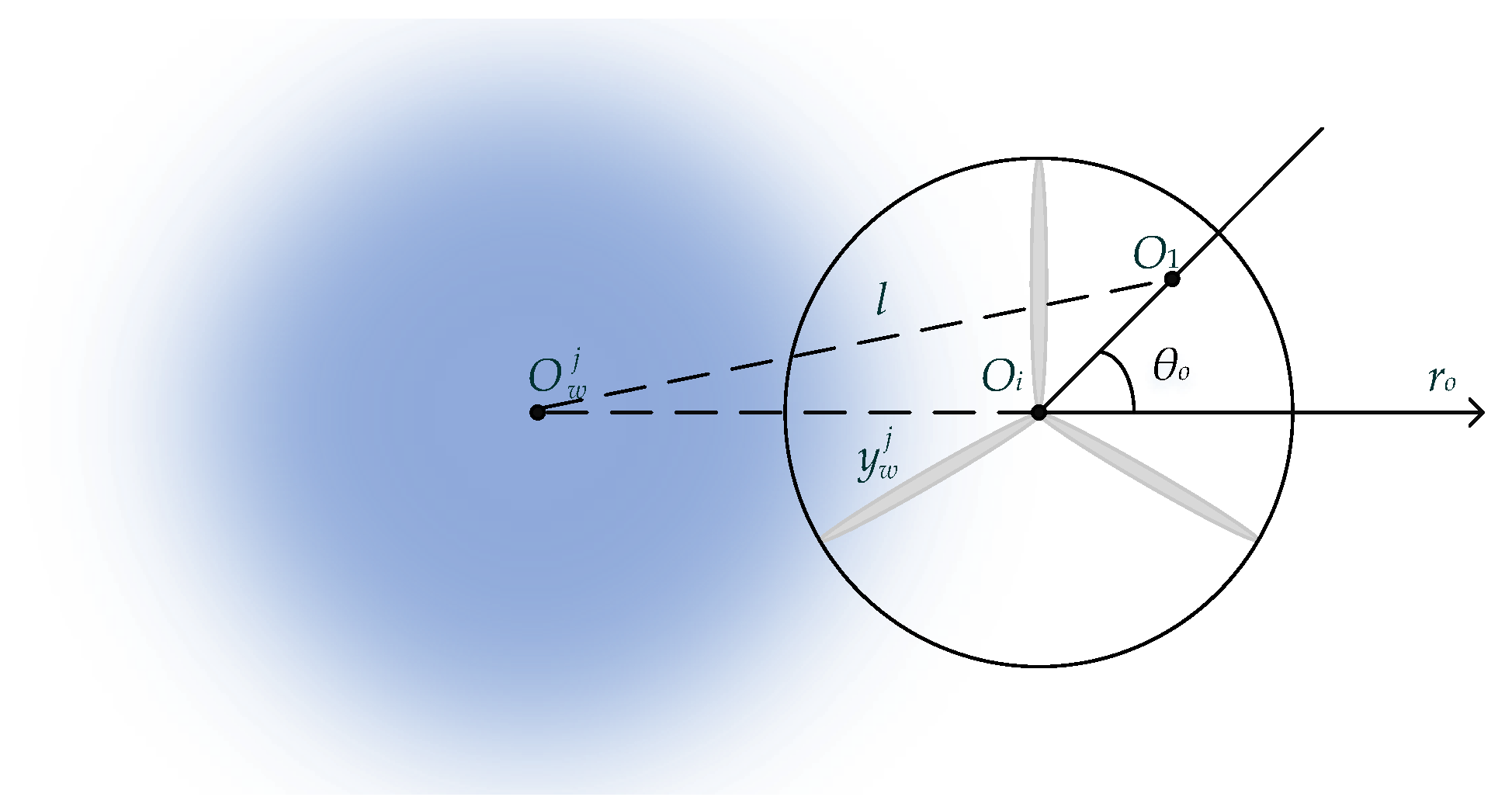
2.2. Single-Wake Model

When there is a yaw misalignment angle between the nacelle centre line and the inflow wind direction, the wake of the wind turbine will deflect sideways. With the yaw misalignment increasing, the deflection will be greater. Figure 1 shows the yawed wake of the ith turbine viewed from above. The calculation of the characteristic parameters of the wake is deduced from the momentum conservation theory. The control volume is established as shown in the area enclosed by the blue lines in Figure 1. The dot-dash line downstream of the turbine is the wake centreline. The magenta dashed lines indicate the boundary of the wake region. The inflow wind speed shown in Figure 1 is aligned with the x-axis direction. We extend the inflow direction to a more general case where there is a deviation angle θ_i between the inflow direction and the x-axis direction. This extension enables the consideration of secondary steering in wake calculations [4]. Then, U_i is decomposed into the x component u_i and the y component v_i:

$$U_i=\left[u_i{,}_{}{v}_i\right]=\left[U_i\cos {\theta }_i,U_i\sin {\theta }_i\right]$$

(7)

According to the established control volume, the momentum equation is as follows:

$$F_i=m_1{U}_d^i+m_2{U}_i-m_3{U}_w^i$$

(8)

where m₁, m₂, and m₃ are, respectively, the mass flow passing through the wind rotor, mixing into the wake region, and crossing the control volume outlet; F_i is the external force acting on the control volume; and $U_w^i$ is the effective wind speed at a downstream section in the wake region. Decomposing $U_d^i$, $U_w^i$, and F_i according to the x-axis direction and the y-axis direction proceeds as follows:

$$U_d^i=\left[u_d^i,v_i\right]=\left[\left(1-a_i\right)u_i,v_i\right]$$

(9)

$$U_w^i=\left[u_w^i,v_w^i\right]$$

(10)

$$F_i=\left[F_x^i,F_y^i\right]$$

(11)

According to Equations (9)–(11), Equation (8) can be rewritten as:

$$F_x^i=\rho \frac{\pi }{4}{D}_i^2\left(1-a_i\right)u_i+\rho \left(\frac{\pi }{4}{\left(D_w^i\right)}^2-\frac{\pi }{4}{D}_i^2\right)u_i-\rho \frac{\pi }{4}{\left(D_w^i\right)}^2{u}_w^i$$

(12)

$$F_y^i=\rho \frac{\pi }{4}{\left(D_w^i\right)}^2\left(v_i-v_w^i\right)$$

(13)

where D_i and $D_w^i$ are the rotor diameter and wake diameter of the ith turbine, respectively; and $u_w^i$ and $v_w^i$ are the streamwise and spanwise wake velocities, respectively. In this work, the inlet of the control volume is placed just behind the rotor to avoid the effect of the thrust force. Thus, F_i is equal to zero. Then, the partial differential equations of (12) and (13) are obtained as follows:

$${\left(D_w^i\right)}^2\left(\frac{\partial u_w^i}{\partial t}+u_i\frac{\partial u_w^i}{\partial x}\right)=2D_w^i{u}_i\frac{\partial D_w^i}{\partial t}+{\left(D_w^i\right)}^2\frac{\partial u_i}{\partial t}-D_i^2{u}_i\frac{\partial a_i}{\partial t}-a_i{D}_i^2\frac{\partial u_i}{\partial t}-2D_w^i{u}_w^i\frac{\partial D_w^i}{\partial t}$$

(14)

$$\frac{\partial v_w^i}{\partial t}+u_i\frac{\partial v_w^i}{\partial x}=\frac{2}{D_w^i}\left(v_i-v_w^i\right)\frac{\partial D_w^i}{\partial t}+\frac{\partial v_i}{\partial t}$$

(15)

The offset distance of the wake centre $y_w^i$ is accumulated by $v_w^i$ against time [24], which means:

$$\frac{\partial y_w^i}{\partial t}+u_i\frac{\partial y_w^i}{\partial x}=v_w^i$$

(16)

In static wake models, the wake diameter typically expands at a fixed rate with downstream distance. In [24], a constant temporal expansion rate k_t was proposed to model the dynamical wake expansion, which is adopted here:

$$\frac{\partial D_w^i}{\partial t}+u_i\frac{\partial D_w^i}{\partial x}=k_t{u}_i$$

(17)

By solving the partial differential Equations (14)–(17), the characteristic parameters of the single-wake model can be obtained. According to the backward difference method, the equations are discretized into the following form to solve:

$$u_w^i\left(x,t\right)=k_{u2}/k_{u1}$$

(18)

$$k_{u1}=\frac{{\left(D_w^i\left(x,t\right)\right)}^2}{T}+\frac{u_i\left(t\right)}{h}+2D_w^i\left(x,t\right)\frac{D_w^i\left(x,t\right)-D_w^i\left(x,t-T\right)}{T}$$

(19)

$$\begin{array}{ll}{k}_{u2}=& \frac{{\left(D_w^i\left(x,t\right)\right)}^2}{T}{u}_w^i\left(x,t-T\right)+\frac{u_i\left(t\right)}{h}{u}_w^i\left(x-h,t\right)+2D_w^i\left(x,t\right)u_i\left(t\right)\frac{D_w^i\left(x,t\right)-D_w^i\left(x,t-T\right)}{T}\\ & {}_{}+\left({\left(D_w^i\left(x,t\right)\right)}^2-a_i\left(t\right)D_i^2\right)\frac{u_i\left(t\right)-u_i\left(t-T\right)}{T}-D_i^2{u}_i\left(t\right)\frac{a_i\left(t\right)-a_i\left(t-T\right)}{T}\end{array}$$

(20)

$$v_w^i\left(x,t\right)=k_{v2}/k_{v1}$$

(21)

$$k_{v1}=\frac{1}{T}+\frac{u_i\left(t\right)}{h}+\frac{2\left(D_w^i\left(x,t\right)-D_w^i\left(x,t-T\right)\right)}{D_w^i\left(x,t\right)T}$$

(22)

$$k_{v2}=\frac{2\left(D_w^i\left(x,t\right)-D_w^i\left(x,t-T\right)\right)}{D_w^i\left(x,t\right)T}{v}_i\left(t\right)+\frac{v_i\left(t\right)-v_i\left(t-T\right)}{T}+\frac{v_w^i\left(x,t-T\right)}{T}+\frac{v_w^i\left(x-h,t\right)}{h}{u}_i\left(t\right)$$

(23)

$$y_w^i(x,t)=\frac{v_w^i\left(x,t\right)+y_w^i(x,t-T)/T+u_i\left(t\right)y_w^i(x-h,t)/h}{1/T+u_i\left(t\right)/h}$$

(24)

$$D_w^i\left(x,t\right)=\frac{k_t+D_w^i\left(x,t-T\right)/T+u_i\left(t\right)D_w^i\left(x-h,t\right)/h}{1/T+u_i\left(t\right)/h}$$

(25)

where T and h are the time step and distance step, respectively; $D_w^i$(x, t) is the wake diameter at time t at the downstream distance x, and other similar variables will not be repeated.

2.3. Initial Conditions

To solve Equations (18)–(25) iteratively, we set the initial conditions at time 0 according to the Jensen wake model [5] as below:

$$\{\begin{array}{l}{y}_w^i\left(x,0\right)=\left(v_i\left(0\right)/u_i\left(0\right)\right)x\hfill \\ u_w^i\left(x,0\right)=u_i\left(0\right)-u_i\left(0\right){\left(a_i{D}_i/\left(D_i/2+k_{x}x\right)\right)}^2\hfill \\ v_w^i\left(x,0\right)=v_i\left(0\right)\hfill \\ D_w^i\left(x,0\right)=D_i+k_{x}x\hfill \end{array}$$

(26)

where k_x is the static wake expansion rate, taken as 0.05 in this study. The initial conditions at x = 0 are set as below [24]:

$$\{\begin{array}{l}{y}_w^i\left(0,t\right)=0\hfill \\ u_w^i\left(0,t\right)=u_{i0}\left(t\right)\hfill \\ v_w^i\left(0,t\right)=v_{i0}\left(t\right)\hfill \\ D_w^i\left(0,t\right)=D_i\hfill \end{array}$$

(27)

$$\left[\begin{array}{c}{u}_{i0}\left(t\right)\\ v_{i0}\left(t\right)\end{array}\right]=\Vert U_i\left(t\right)\Vert \left(1-a_i\left(t\right)\right)\left[\begin{array}{c}\cos \left({\xi }_{w0}^i\left(t\right)+{\theta }_i\left(t\right)\right)\\ \sin \left({\xi }_{w0}^i\left(t\right)+{\theta }_i\left(t\right)\right)\end{array}\right]$$

(28)

where ${\xi }_{w0}^i$(t) is the wake skew angle at x = 0, which is calculated as below [8]:

$${\xi }_{w0}^i\left(t\right)=C_t^i\left(t\right){\cos }^2{\gamma }_i\left(t\right)\sin {\gamma }_i\left(t\right)/2$$

(29)

2.4. Modifications of Single-Wake Model

The single-wake model in Section 2.2 simplifies the spanwise of the wake velocity to a top-hat shape distribution. A super-Gaussian model is applied here to modify the top-hat shape distribution for higher accuracy. In the super-Gaussian model shown in (30), n is a positive integer. The larger n is, the closer the distribution is to a top-hat shape distribution [42]. When n = 2, the distribution is a Gaussian shape.

$$g\left(r\right)=\frac{1}{\sqrt{2\pi }{\sigma }_0}\exp \left(\frac{-r^n}{2{\sigma }_0^n}\right)$$

(30)

where σ₀ is the characteristic wake width, which has the following transformation relationship with the standard deviation σ of Gaussian distribution:

$$\sigma ={\sigma }_0{\left(\pi /2\right)}^{2/n-1}$$

(31)

For the requirement that the momentum deficit of the wake flow per unit length in the x-direction is the same as the original top-hat shape distribution, the spanwise distribution of the wake velocity in Section 2.2 is modified to a super-Gaussian shape as below:

$$\{\begin{array}{l}{\stackrel{⌣}{U}}_w^i\left(x,t,r\right)=U_i\left(t\right)-U_i\left(t\right)C\left(x\right)\exp \left(-r^n/\left(2{\sigma }_0^n\right)\right)\hfill \\ C\left(x\right)=\frac{n\left(U_i\left(t\right)-U_w^i\left(x,t\right)\right)D_w^i{\left(x,t\right)}^2{\left(1/\left(2{\sigma }_0^n\right)\right)}^{2/n}}{8U_i\left(t\right)\mathrm{\Gamma }\left(2/n\right)}\hfill \end{array}$$

(32)

where ${\stackrel{⌣}{U}}_w^i\left(x,t,r\right)$ is the wake velocity at a spanwise distance r from the wake centre at time t, while the wake centre is at a distance x downstream of turbine i; C(x) is the maximum velocity deficit, of which the derivation process is listed in Appendix A; Γ(.) is the Gamma function. To determine σ₀, σ takes a value as:

$$\sigma \left(x,t\right)=D_w^i(x,t)/\left(4\sqrt{\ln 2}\right)$$

(33)

By doing this, over 95% of the momentum loss is distributed within a circle of radius $D_w^i$/2 around the wake centre.

In addition, due to the wake expansion effect, the spanwise velocity induced by the wind rotor will gradually decrease along the flow direction [43]. This means that as x increases, $y_w^i$ will gradually tend to be constant. In [11], Qian and Ishihara proposed a Gaussian-based wake model and compared the wake centreline offset of the Gaussian-based model with the Jimenez wake deflection model [8] and wind tunnel experimental data. The results showed that the Jimenez wake deflection model generally overestimated the wake deflections under different yaw angles, while the Gaussian-based model agreed well with the experimental data. Therefore, this paper selects the wake offset of the Gaussian-based model proposed by Qian and Ishihara as a more reliable basis. To ensure the technical accuracy of the model, we establish that spanwise velocity decay should begin at 6D to allow the model’s wake offset to agree well with the Gaussian-based model. Therefore, (21) is empirically modified as below:

$$v_w^i\left(x,t\right)=\{\begin{array}{l}{k}_{v2}/k_{v1}{,}_{}x\le 6D_i\hfill \\ {\left(x-6D_i\right)}^{-1}{k}_{v2}/k_{v1}{,}_{}x>6D_i\hfill \end{array}$$

(34)

After the modification, the spanwise wake velocity $v_w^i$ will gradually decay to 0 when x is greater than 6D_i.

2.5. Wake Interaction

Figure 2 shows the wake interaction between an upstream turbine j and a downstream turbine i. The blue shaded area is the wake section of turbine j at the downstream distance of turbine i, and $O_w^j$ is the centre of the wake section. The black circle represents the rotor plane of turbine i, and O_i is its centre. $y_w^j$ is the distance between $O_w^j$ and O_i. O₁ (r_o, θ_o) is a random point inside the rotor plane. l is the distance between $O_w^j$ and O₁, which is calculated as:

$$l\left(r_o,{\theta }_o\right)=\sqrt{{\left(y_w^j\right)}^2+r_o^2-2y_w^j{r}_o\cos \left(\pi -{\theta }_o\right)}$$

(35)

Establishing a polar coordinate system as shown in Figure 2 and setting the pole at O_i, we obtain the effective wind speed U_ij of turbine i under the wake of turbine j as below:

$$U_{ij}\left(t\right)={\displaystyle {\int }_0^{2\pi }{\displaystyle {\int }_0^{D_i/2}{r}_o{\stackrel{⌣}{U}}_w^j\left(l\left(r_o,{\theta }_o\right),t\right)d{r}_{o}d{\theta }_o}}/\left(\pi D_i^2/4\right)$$

(36)

In wind farms, a downstream turbine is usually affected by the wakes of multiple upstream turbines to varying degrees. The effect of multi-wakes on the turbine needs to be superimposed equivalently. Several wake superposition methods have been proposed [37]. The rotor-based root sum square method is applied here to calculate the effective wind speed U_i of the ith downstream turbine [44]:

$$U_i=U_{\infty }-\sqrt{{\displaystyle {\sum }_{k=1}^m{\left(U_j-U_{ij}\right)}^2}}$$

(37)

where U_∞ is the free-stream wind speed unaffected by wakes; m is the number of upstream turbines with wake effect on turbine i; U_j is the inflow wind speed of an upstream turbine j.

3. Model Validation

The proposed dynamic wake model in Section 2 is validated in this section by multiple comparative analyses, including the comparison with widely accepted static wake models and the comparison with the dynamic calculation results from SOWFA. Relevant parameters are set as: T = 1 s, h = 1 m, k_t = 0.08, n = 8.

3.1. Comparison of Static Wake Distributions

In this section, we first verify the static characteristics of the proposed dynamic model (Dyn-model). To this end, the results after stabilization will be compared with the results of two static wake models from the FLORIS modelling tool [45]. The first static model for comparison is the well-known Jensen wake model [5]. The other static model is an improved Gaussian-based wake model proposed by Qian and Ishihara in [11] and [10].

The simulation is based on a DTU 10MW wind turbine, of which the rotor diameter D is 178.3 m. More parameters of DTU 10MW turbine are in [46]. The free-stream wind speed is set to U_∞ = 10 m/s, and the axial induction factor is set to a = 1/3. The distributions of the dynamic wake are taken at 600 s when the wake is fully developed and stable. As shown in Figure 1, a coordinate system is established at the location of the turbine. The wake velocity distributions of the turbine at 0°, 10°, 20°, and 30° yaw misalignment are shown in Figure 3.

As can be seen in Figure 3, when the yaw misalignment γ is 0°, the wake deficit distributions of the three models are close. In more detail, the overall wake deficit of the dynamic model is closer to the Jensen model and higher than the Gaussian-based model. This is because the momentum conservation method used in the dynamic wake derivation is the same as that utilized in the Jensen model. The wake deficits of the dynamic model are distributed in a super-Gaussian shape. The Jensen model is unavailable in yawed states. In [39], it was combined with the Jimenez wake deflection model [8] for yawed states. This combination is applied here when yaw misalignment is 10°, 20°, and 30°. In yawed states, the wake centrelines of the dynamic model under different yaw settings agree well with the Gaussian-based model, though the wake velocity deficit is higher than it. The overall wake deficit of the dynamic model is still closer to the combined Jensen model. Also,

Table 1. Wake velocity deficit at different downstream distances (γ = 10°, ×10⁵ m/s∙m²).

	2D	4D	6D	8D	10D
Gaussian-based model	1.0719	1.0719	1.0719	1.0719	1.0719
Jensen model	1.6639	1.6639	1.6640	1.6641	1.6641
Dyn-model	1.6668	1.6677	1.6681	1.6682	1.6682

shows the amount of wake velocity deficit at different downstream distances of the three wake models when γ = 10°. It can be seen that the results of the Jensen model and Dyn-model are very close, while the Gaussian-based model relatively underestimates the overall wake deficit. This phenomenon holds for different yaw angles.

For all the three models, the offset of the wake centreline is more obvious with increasing yaw deviation. When x is greater than 6D, the offset of the wake centrelines of the dynamic model and the Gaussian-based model hardly increase. The centreline offset of the combined Jensen model is greater than that of the other two models under different yaw angles, while the wake deviations calculated by the proposed wake model always agree well with the Gaussian-based model. In [11], the wake centreline offset of the Gaussian-based wake model has been validated through wind tunnel experimental data. This indirectly validates the proposed wake model’s ability to accurately predict wake deviation.

To verify the time-varying process of the dynamic wake model, dynamic yaw simulations based on the Dyn-model and the combined Jensen model are conducted on a single row of two DTU 10 MW turbines, as shown in Figure 4a. The results are compared with the results reported in [20], which are obtained from SOWFA, a high-fidelity simulation tool. Other parameters are also set according to the case in [20]: the turbines are aligned with the free-stream wind speed at a 5D interval; the free-stream wind speed is set to U_∞ = 9 m/s and kept constant; the yaw angle variation of the upstream turbine is set as shown in Figure 4b, while the downstream turbine remains unyawed during the simulation. Each time the yaw angle is adjusted, it changes continuously at a rate of 1°.s⁻¹.

3.2. Validation of Dynamic Wake

Figure 5 displays the time-varying characteristic parameters of the upstream turbine of the Dyn-model, including $u_w^i$, $v_w^i$, $y_w^i$, and σ₀ at any downstream distance from 0 to 5D during the simulation. As mentioned in Section 2.3, the wake is distributed according to the Jensen model as the initial condition when t = 0 s. At that moment, $u_w^i$ gradually recovers with increasing downstream distance, and σ₀ expands linearly; $v_w^i$ and $y_w^i$ are 0 along with the downstream distance, as the vertical component of the free-stream wind speed is 0. The yaw setting changes over time thereafter. As shown in Figure 5a,d, the distributions of $u_w^i$ and σ₀ are not affected by the yaw angle and are in close agreement with the distributions of the Jensen model. Moreover, $v_w^i$ increases with yaw amplitude, and its value does not change with the downstream distance, as shown in Figure 5b. Accordingly, $y_w^i$ increases with yaw amplitude and downstream distance.

The power output is compared as shown in Figure 6. As the yaw angle increases, the power output of the upstream turbine P₁ decreases rapidly in both cases. Meanwhile, the power output of the downstream turbine P₂ increases with a larger yaw angle. Due to the delay in wake propagation, there is a time lag between the variation of the downstream turbine and the upstream one. It can be seen that the time lag described by the Dyn-model is in close agreement with that of SOWFA. As a static model, the combined Jensen model failed to reflect the time lag. Moreover, the power outputs of the upstream turbine in all cases are close. For the downstream turbine, even ignoring the time lag, the power output calculated by the Dyn-model is still closer to SOWFA than the combined Jensen model. For the same yaw angle of the upstream turbine, P₂ calculated by the combined Jensen model will be greater than that calculated by the Dyn-model. This phenomenon can be explained by the excessive yaw deflection estimated by the Jimenez wake deflection model. Due to the overestimated wake deflection, the wake deficit of the downstream turbine will be underestimated.

Then, another dynamic yaw simulation is carried out on the dynamic wake model, with the same layout as shown in Figure 4a and U_∞ = 9 m/s. The yaw setting of the upstream turbine is displayed in Figure 7. Each time sample T_k in Figure 4 represents a time interval of 2 s. To compare the wake development process of the Dyn-model with SOWFA, the wake velocity distributions in the range of 0–5D downstream of the upstream turbine at some time samples are shown in Figure 8. The compared results of SOWFA are also reported in [20]. The selected time samples are T_k = 410, 430, 450, 470, 490. The yaw angles at these moments are displayed in the enlarged view of Figure 7.

In Figure 8, the left column shows the wake distributions calculated by SOWFA, and the right column displays the corresponding distributions of the Dyn-model. When T_k = 410, the yaw angle is about to gradually change from 0° to −20°, and no significant wake deflection can be observed in either case. The yaw angle reaches −20° when T_k = 417, after which the −20° yawed wake propagates backward. The −20° yawed wake develops to a position about 250 m downstream of the upstream turbine when T_k = 430, and it then develops to a position about 550 m downstream when T_k = 450. The yaw angle returns to 0° when T_k = 467, after which the new unyawed wake develops downstream again. When T_k = 470, the −20° yawed wake develops a position close to 800 m downstream (the Dyn-model develops slightly faster), and the unyawed wake develops to a position of about 80 m downstream. When T_k = 470, the 5D downstream position is covered by the −20° yawed wake, while the unyawed wake develops to a position of about 320 m downstream. In general, the wake development process of the Dyn-model is close to that of SOWFA. In addition, the Dyn-model underestimates the near-wake wind speed compared with SOWFA. In the far wake region, the wind speed of the Dyn-model is close to that of SOWFA. Since the distance between turbines in a wind farm is usually large to reduce wake losses, the accuracy of the far wake region is more of a concern. Moreover, it can be seen from the Figure 8 that the yawed wake deviations calculated by the proposed model at different moments are in good agreement with the results calculated by SOWFA.

In summary, the dynamic wake model proposed in this study has a static wake distribution that is close to the accuracy of the common control-oriented wake models, i.e., the Jensen model and the Gaussian-based model. At the same time, the wake delay during the dynamic simulation process is close to the result of the high-precision computational fluid dynamics (CFD) software, SOWFA.

4. Wind Farm Production Maximisation Based on Dynamic Yawed Wake Calculation

In this section, we first analyse the influence of wake propagation time lag on wind farm yaw control, and then explore a yaw optimisation method for increasing wind farm energy capture based on the dynamic wake model. As shown in Figure 9, case studies in this section are based on a single row of five turbines with a diameter D₁ of 100 m. The distance between two adjacent turbines is 5D₁.

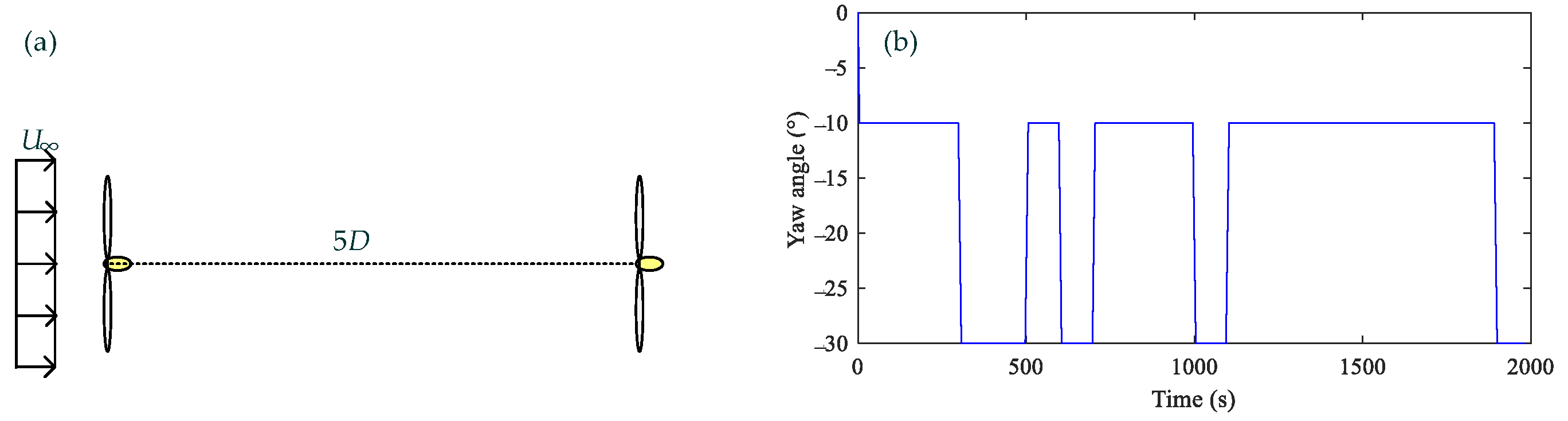
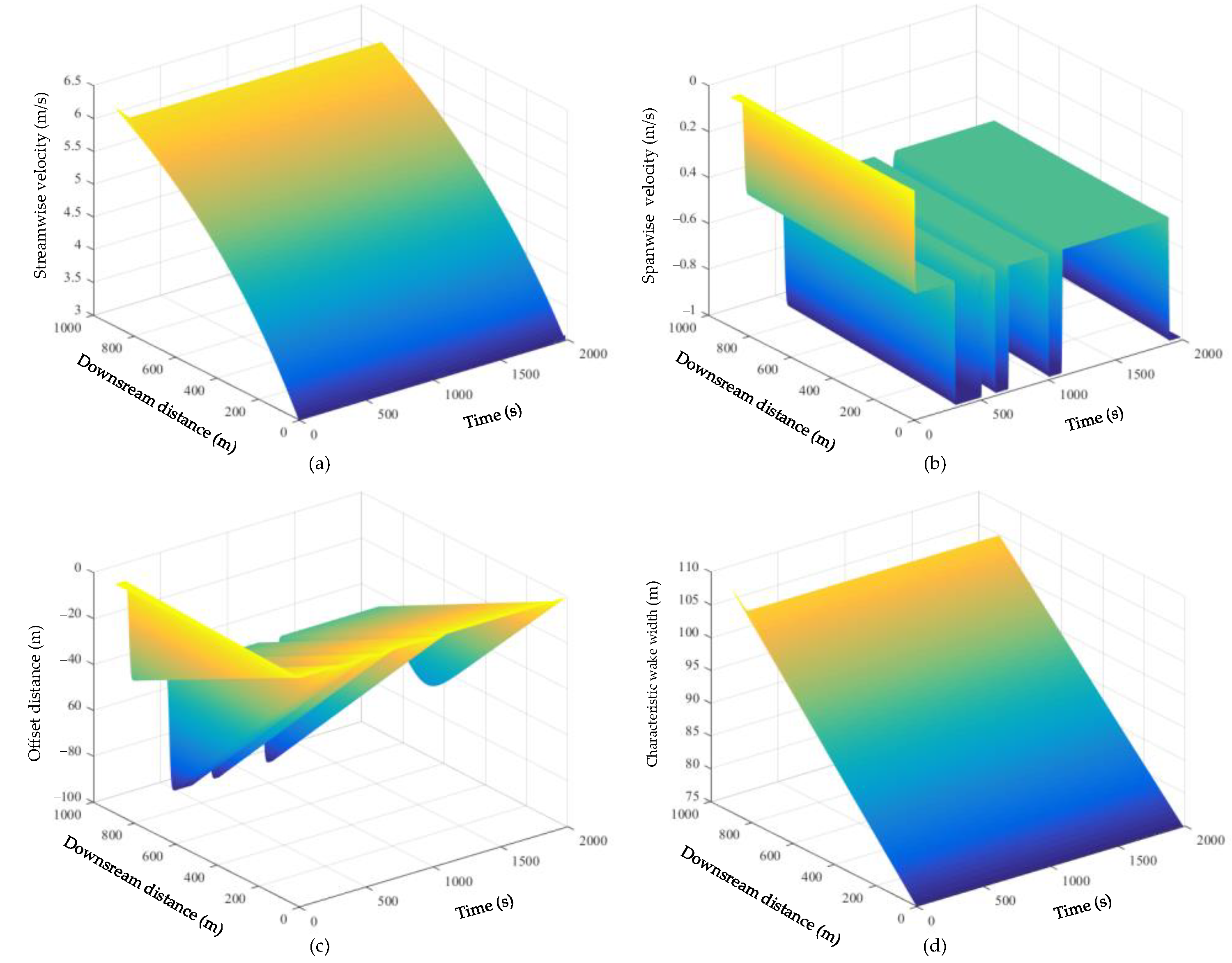
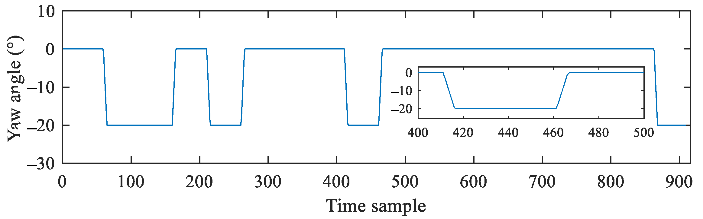
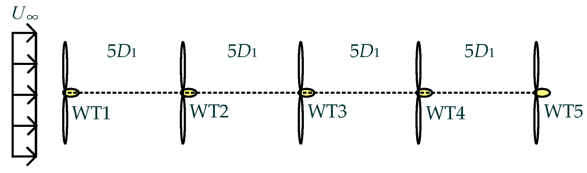
4.1. Wake Propagation

The free-stream wind speed is set to U_∞ = 10 m/s. The yaw misalignment of the most upstream turbine (WT1) γ₁ is set to 0° and 30°, while the downstream turbines remain unyawed during the simulation. The effective wind speed of each turbine under different yaw settings of WT1 is shown in Figure 10. For about the first 50 s, different yaw settings do not affect the wind speed of the downstream turbines. Subsequently, the wind speed of each downstream turbine begins to change and converges to a higher value. Moreover, the further downstream the turbine is, the longer it takes for its wind speed to converge to the higher value. This phenomenon can be explained by the time lag of wake propagation, which is instructive for increasing wind farm production through wake regulation. Moreover, it can be seen that u₃, u₄, and u₅ first drop and then rise back. When calculating the effective wind speed of the downstream turbine through wake superposition, the effective wind speed of the downstream turbine will decrease with the increase of the effective wind speed of the upstream turbine. However, when the yaw wake continues to propagate to the downstream turbine, its wind speed rises back. It can be seen from u₄ and u₅ that the effective wind speed drop of the downstream turbine is mainly affected by the adjacent upstream turbine.

To further understand the impact of wake propagation on wind farm production maximisation, another simulation experiment is conducted. The free-stream wind speeds of two sequential simulation periods are assumed to be constant during each period and set as U_∞ = [8, 10]. The optimisation period T_c is set as 100 s. As shown in Figure 11a, three scenarios are set according to different yaw settings of WT1. The downstream turbines remain unyawed. The wind farm electrical energy outputs in each optimisation period under different scenarios are shown in Figure 11b. During period 1, WT1 remains unyawed in Scenario 1, while it performs a 30° yaw misalignment in Scenarios 2 and 3. This results in a lower wind farm electrical energy output for Scenarios 2 and 3 than Scenario 1 in period 1. This is because in Scenarios 2 and 3, the power output of WT1 decreases immediately after yaw, but the yaw wake has not yet propagated to WT2 during period 1 to increase the power output of WT2.

During period 2, WT1 remains unyawed in Scenarios 1 and 2, and performs a 30° yaw misalignment in Scenario 3. As a result, the relationship between the energy output of the three scenarios is: Scenario2 > Scenario 3 > Scenario 1. The results can be explained by the fact that, in Scenario 2, WT1 does not yaw during period 2, so its power does not drop. Meanwhile, the yaw wake caused by the yaw action of WT1 in period 1 reaches WT2 in period 2 due to the propagation time lag, so that the power of WT2 increases in period 2. In Scenario 3, although the yaw action of WT1 in period 1 also caused the power increase of WT2 in period 2, WT1 keeps yawing in period 2, causing its own power to decrease. Moreover, the yaw wake in period 2 has not yet reached WT2. Therefore, the power generation of Scenario 3 is less than that of Scenario 2. In Scenario 1, WT1 remains unyawed in periods 1 and 2, so the power of WT2 does not increase in period 2 while the power of WT1 does not decrease. Due to the fact that the yaw of WT1 causes the power increase of WT2 to be larger than its own power decrease, the overall power of Scenario 1 is less than that of Scenario 3.

Overall, two time periods are crucial for increasing the power generation of wind farms by wake offset. The first is the time lag from the yaw operation of the upstream turbine to when the wake starts to deviate from downstream turbines. The second is the time for the increased power of downstream turbines through wake offset to compensate for the decreased power of the yawed turbine. When the optimisation period is too short, the yaw operation may not lead to the production increase of the wind farm within one period and may cause a production increase in the subsequent period.

4.2. Wind Farm Production Maximisation Based on Dynamic Wake Model

Based on the proposed dynamic wake model, a yaw optimisation method for increasing wind farm energy capture is present here.

4.2.1. Problem Statement

Wind farm production maximisation based on static wake models usually takes wind farm power P_wf as the optimisation objective. Such an objective is not feasible for the optimisation based on a dynamic wake model, because the power output of the wind farm is constantly changing in the dynamic calculation. In this study, we take the generated electrical energy E_wf of the wind farm within one optimisation period as the optimisation objective and use the proposed dynamic wake model for wind farm prediction. Therefore, the optimisation problem is formulated as below [40]:

$$\begin{gathered} \begin{array}{cc}{\max }_{}{E}_{wf}\left(U,a,\gamma \right)\hfill & ={\displaystyle {\sum }_{i=1}^5{E}_i\left(U_i,a_i,{\gamma }_i\right)}\hfill \\ & ={\displaystyle {\sum }_{i=1}^5{\displaystyle \int P_i}}\left(U_i,a_i,{\gamma }_i\right)dt\hfill \end{array} \\ \mathrm{s}.\mathrm{t}{.}_{}{\gamma }_{\min }^i\le {\gamma }_i\le {\gamma }_{\max }^i{,}_{}i=1,2,\cdots ,5 \end{gathered}$$

(38)

where E_i is the generated electrical energy of turbine i within one optimisation period; P_i is the power output of turbine i at time t, which is calculated according to Equations (1) and (4). The optimisation variables are the yaw angles of each turbine γ = [γ₁, γ₂,⋯,γ₅]. Constraints on the yaw misalignment angles of the turbines are considered. According to previous studies [35,47], positive yaw misalignment angles (yaw counterclockwise) are more efficient in achieving wind farm power increases in the northern hemisphere, due to the effect of the Coriolis force. Thus, we set: ${\gamma }_{min}^i$ = 0°, ${\gamma }_{max}^i$ = 30°. During the optimisation process, the axial induction factor of each turbine is set to a_i = 1/3.

4.2.2. Optimisation Results

The problem described in Equation (38) is an uncomplicated optimisation problem with low dimensions. The particle swarm optimisation (PSO) method is widely utilized in wind farm optimisation problems [28]. A stochastic PSO method is applied here to solve the problem (38). The number of particles is set to 20, and the number of iterations is set to 50. The cognitive and social parameters are set to c₁ = c₂ = 2. More details of the stochastic PSO omitted here can be found in [48], as the solution method is not the focus of this paper. The free-stream wind speed of each optimisation period is assumed to be constant. Then, the free-stream wind speeds of ten sequential simulation periods are set as U_∞ = {6, 8, 10, 9, 5, 7, 9, 11, 10, 8}. Different wake models have different emphases and precisions. Therefore, it is difficult to directly compare the wake control effects of different wake models. Researchers often rely on high-precision fluid simulations for third-party comparisons. This study focuses on exploring wake regulation for wind farm production maximisation considering wake propagation and is limited by high-precision fluid simulation conditions. Thus, the results under different optimisation period settings are compared with those under the maximum power point tracking (MPPT) strategy based on the proposed dynamic wake model.

Under different period lengths of 100 s, 300 s, and 600 s, respectively, the generated electrical energy of the wind farm and the optimised yaw settings of each turbine in each period are shown in Figure 12. It is apparent that with a longer period or higher free-stream wind speed, the energy production increase of the wind farm is more obvious. When T_c is set to 100 s, all turbines remain unyawed. According to the analysis in Section 4.1, it is because the increased energy of downstream turbines through wake offset is not enough to compensate for the decreased power of the yawed turbines within one period. As shown in Figure 12c,e, the first period has a lower energy increase than all subsequent periods. This is because the wind turbines are still affected by the yawed wakes of the previous period at the beginning of a subsequent period, while the yaw wakes in the first period have not fully developed to the downstream turbines.

As the wind speed increases, the yaw wake reaches the downstream turbines faster. Therefore, the wake optimisation at a high wind speed can be set for a shorter regulation period. This study explores a more general period length for different wind speeds. To this end, the increases of the wind farm energy during all the ten periods under different period lengths are shown in Figure 13. It can be seen that after Tc is greater than 300 s, the effect of extending the period length on energy increment is no longer obvious. Moreover, control accuracy degrades with a longer optimisation period length. Thus, 300 s should be a suitable period length for wind farm production maximisation based on the dynamic wake model.

5. Conclusions

This study develops a simplified dynamic wake model capable of simulating the time-varying process of wake propagation. Based on the dynamic wake model, a wind farm production maximisation method through yaw optimisation is proposed, considering the time lag of wake propagation. The main conclusions of this research are as below:

• A simplified dynamic wake model for wind farm prediction is derived according to the momentum conservation theory and backward difference method. The spanwise velocity deficit of the wake is based on super-Gaussian distribution. The wake superposition is conducted by the rotor-based root sum square method.
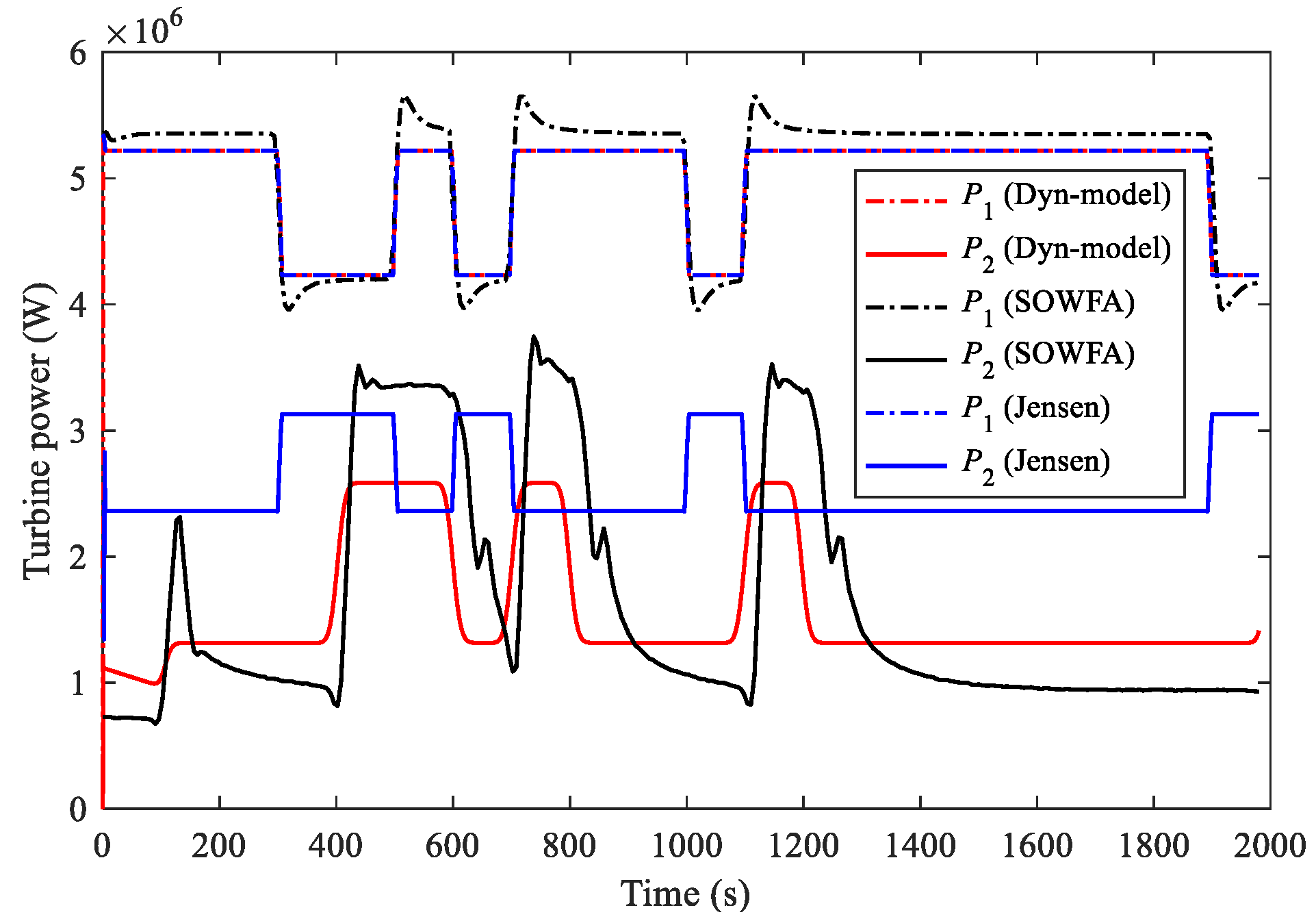
• The static distribution of the proposed model is validated with the Jensen model and a Gaussian-based static model. The time-varying process of the proposed model agrees well with numerical results from SOWFA.
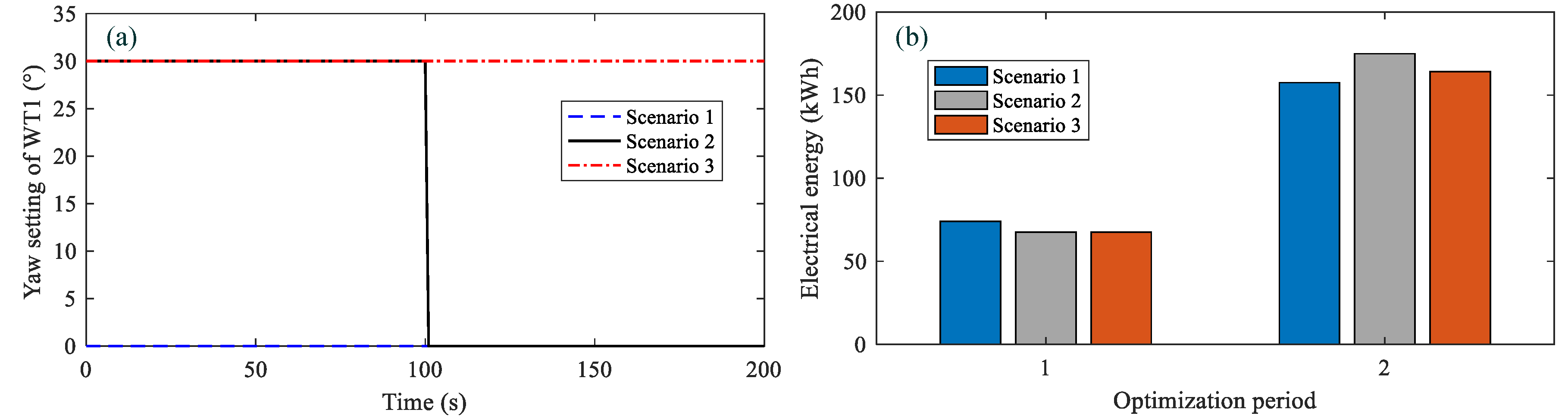
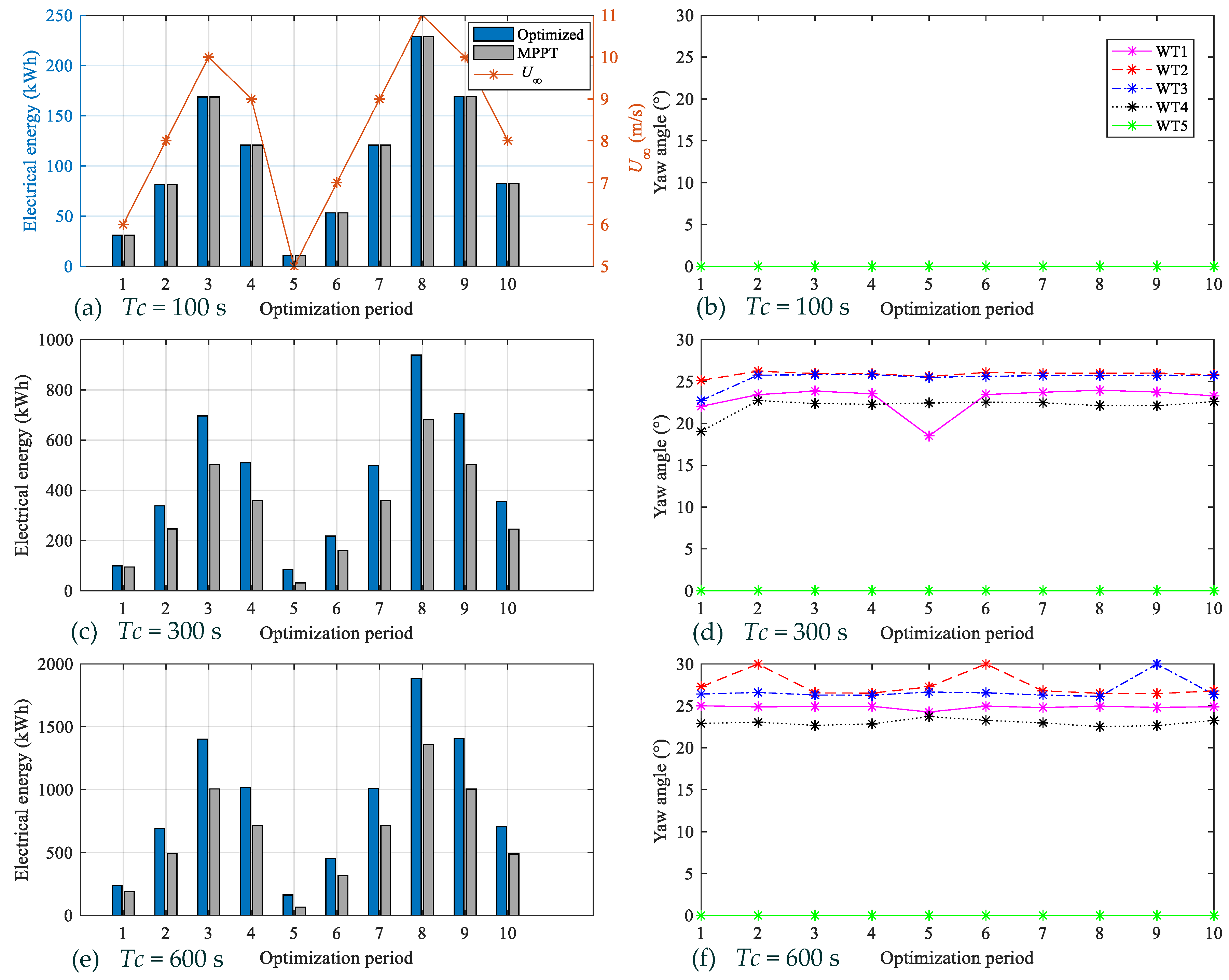
• The wind farm production maximisation through wake meandering is analysed from the perspective of dynamic wake calculation. Different from the optimisation methods based on a static wake model, the increase in wind farm production is closely related to the optimisation period length, due to the time lag of wake propagation.

In the future, better optimisation methods for increasing wind farm energy capture could be explored considering the time-varying wake. Moreover, as can be seen from the results in Section 3.2, the downstream turbine power calculated by the proposed wake model in this paper is still somewhat in error with that of SOWFA. Further research will be conducted to improve the accuracy of the proposed wake model.

References

1. Poudyal, R.; Loskot, P.; Nepal, R.; Parajuli, R.; Khadka, S.K. Mitigating the current energy crisis in Nepal with renewable energy sources. Renew. Sustain. Energy Rev. 2019, 116, 109388. [Google Scholar] [CrossRef]
2. Gu, B.; Meng, H.; Ge, M.; Zhang, H.; Liu, X. Cooperative multiagent optimization method for wind farm power delivery maximization. Energy 2021, 233, 121076. [Google Scholar] [CrossRef]
3. Khan, M.A.; Javed, A.; Shakir, S.; Syed, A.H. Optimization of a wind farm by coupled actuator disk and mesoscale models to mitigate neighboring wind farm wake interference from repowering perspective. Appl. Energy 2021, 298, 117229. [Google Scholar] [CrossRef]
4. Kheirabadi, A.C.; Nagamune, R. A quantitative review of wind farm control with the objective of wind farm power maximization. J. Wind. Eng. Ind. Aerodyn. 2019, 192, 45–73. [Google Scholar] [CrossRef]
5. Jensen, N. A Note on Wind Generator Interaction; Risø National Laboratory: Roskilde, Denmark, 1983. [Google Scholar]
6. Frandsen, S.; Barthelmie, R.; Pryor, S.; Rathmann, O.; Larsen, S.; Højstrup, J.; Thøgersen, M. Analytical modelling of wind speed deficit in large offshore wind farms. Wind. Energy 2006, 9, 39–53. [Google Scholar] [CrossRef]
7. Katic, I.; Højstrup, J.; Jensen, N. A simple model for cluster efficiency. In European Wind Energy Association Conference and Exhibition; Raguzzi, A., Ed.; Rome, Italy, 1986; Volume 1l, pp. 407–410. [Google Scholar]
8. Jiménez, Á.; Crespo, A.; Migoya, E. Application of a LES technique to characterize the wake deflection of a wind turbine in yaw. Wind. Energy 2009, 13, 559–572. [Google Scholar] [CrossRef]
9. Bastankhah, M.; Porté-Agel, F. Experimental and theoretical study of wind turbine wakes in yawed conditions. J. Fluid Mech. 2016, 806, 506–541. [Google Scholar] [CrossRef]
10. Ishihara, T.; Qian, G.-W. A new Gaussian-based analytical wake model for wind turbines considering ambient turbulence intensities and thrust coefficient effects. J. Wind. Eng. Ind. Aerodyn. 2018, 177, 275–292. [Google Scholar] [CrossRef]
11. Qian, G.-W.; Ishihara, T. A New Analytical Wake Model for Yawed Wind Turbines. Energies 2018, 11, 665. [Google Scholar] [CrossRef]
12. Blondel, F.; Cathelain, M. An alternative form of the super-Gaussian wind turbine wake model. Wind. Energy Sci. 2020, 5, 1225–1236. [Google Scholar] [CrossRef]
13. Zong, H.; Porté-Agel, F. Experimental investigation and analytical modelling of active yaw control for wind farm power optimization. Renew. Energy 2021, 170, 1228–1244. [Google Scholar] [CrossRef]
14. Lin, J.W.; Zhu, W.J.; Shen, W.Z. New engineering wake model for wind farm applications. Renew. Energy 2022, 198, 1354–1363. [Google Scholar] [CrossRef]
15. Martínez-Tossas, L.A.; Annoni, J.; Fleming, P.A.; Churchfield, M.J. The aerodynamics of the curled wake: A simplified model in view of flow control. Wind. Energy Sci. 2019, 4, 127–138. [Google Scholar] [CrossRef]
16. Dou, B.; Qu, T.; Lei, L.; Zeng, P. Optimization of wind turbine yaw angles in a wind farm using a three-dimensional yawed wake model. Energy 2020, 209, 118415. [Google Scholar] [CrossRef]
17. Zhang, J.; Zhao, X. A novel dynamic wind farm wake model based on deep learning. Appl. Energy 2020, 277, 115552. [Google Scholar] [CrossRef]
18. Chen, H.; Staupe-Delgado, R. Exploiting more robust and efficacious deep learning techniques for modeling wind power with speed. Energy Rep. 2022, 8, 864–870. [Google Scholar] [CrossRef]
19. Cassamo, N.; van Wingerden, J.-W. On the Potential of Reduced Order Models for Wind Farm Control: A Koopman Dynamic Mode Decomposition Approach. Energies 2020, 13, 6513. [Google Scholar] [CrossRef]
20. Cassamo, N.R. Model Predictive Control for Wake Steering: A Koopman Dynamic Mode Decomposition Approach; University of Lisbon: Lisbon, Portugal, 2020. [Google Scholar]
21. Fortes-Plaza, A.; Campagnolo, F.; Wang, J.; Wang, C.; Bottasso, C.L. A POD reduced-order model for wake steering control. J. Phys. Conf. Ser. 2018, 1037, 032014. [Google Scholar] [CrossRef]
22. Gebraad, P.M.O.; van Wingerden, J.W. A Control-Oriented Dynamic Model for Wakes in Wind Plants. J. Phys. Conf. Ser. 2014, 524, 012186. [Google Scholar] [CrossRef]
23. Gebraad, P.M.O.; Fleming, P.A.; van Wingerden, J.W. Wind turbine wake estimation and control using FLORIDyn, a control-oriented dynamic wind plant model. In Proceedings of the 2015 American Control Conference (ACC), Chicago, IL, USA, 1–3 July 2015; Volume 2015, pp. 1702–1708. [Google Scholar]
24. Kheirabadi, A.C.; Nagamune, R. A low-fidelity dynamic wind farm model for simulating time-varying wind conditions and floating platform motion. Ocean. Eng. 2021, 234, 109313. [Google Scholar] [CrossRef]
25. Boersma, S.; Doekemeijer, B.; Vali, M.; Meyers, J.; van Wingerden, J.-W. A control-oriented dynamic wind farm model: WFSim. Wind. Energy Sci. 2018, 3, 75–95. [Google Scholar] [CrossRef]
26. Nash, R.; Nouri, R.; Vasel-Be-Hagh, A. Wind turbine wake control strategies: A review and concept proposal. Energy Convers. Manag. 2021, 245, 114581. [Google Scholar] [CrossRef]
27. Shen, Y.; Xiao, T.; Lv, Q.; Zhang, X.; Zhang, Y.; Wang, Y.; Wu, J. Coordinated optimal control of active power of wind farms considering wake effect. Energy Rep. 2022, 8, 84–90. [Google Scholar] [CrossRef]
28. Gionfra, N.; Sandou, G.; Siguerdidjane, H.; Faille, D.; Loevenbruck, P. Wind farm distributed PSO-based control for constrained power generation maximization. Renew. Energy 2019, 133, 103–117. [Google Scholar] [CrossRef]
29. Lin, M.; Porté-Agel, F. Power Production and Blade Fatigue of a Wind Turbine Array Subjected to Active Yaw Control. Energies 2023, 16, 2542. [Google Scholar] [CrossRef]
30. Annoni, J.; Gebraad, P.M.O.; Scholbrock, A.K.; Fleming, P.A.; van Wingerden, J.W. Analysis of axial-induction-based wind plant control using an engineering and a high-order wind plant model. Wind Energy 2015, 19, 1135–1150. [Google Scholar] [CrossRef]
31. Munters, W.; Meyers, J. Towards practical dynamic induction control of wind farms: Analysis of optimally controlled wind-farm boundary layers and sinusoidal induction control of first-row turbines. Wind. Energy Sci. 2018, 3, 409–425. [Google Scholar] [CrossRef]
32. Kheirabadi, A.C.; Nagamune, R. Real-time relocation of floating offshore wind turbine platforms for wind farm efficiency maximization: An assessment of feasibility and steady-state potential. Ocean. Eng. 2020, 208, 107445. [Google Scholar] [CrossRef]
33. Fleming, P.; King, J.; Simley, E.; Roadman, J.; Scholbrock, A.; Murphy, P.; Lundquist, J.K.; Moriarty, P.; Fleming, K.; van Dam, J.; et al. Continued results from a field campaign of wake steering applied at a commercial wind farm—Part 2. Wind. Energy Sci. 2020, 5, 945–958. [Google Scholar] [CrossRef]
34. Doekemeijer, B.M.; Kern, S.; Maturu, S.; Kanev, S.; Salbert, B.; Schreiber, J.; Campagnolo, F.; Bottasso, C.L.; Schuler, S.; Wilts, F.; et al. Field experiment for open-loop yaw-based wake steering at a commercial onshore wind farm in Italy. Wind. Energy Sci. 2021, 6, 159–176. [Google Scholar] [CrossRef]
35. Archer, C.L.; Vasel-Be-Hagh, A. Wake steering via yaw control in multi-turbine wind farms: Recommendations based on large-eddy simulation. Sustain. Energy Technol. Assess. 2019, 33, 34–43. [Google Scholar] [CrossRef]
36. Doekemeijer, B.M.; van der Hoek, D.; van Wingerden, J.-W. Closed-loop model-based wind farm control using FLORIS under time-varying inflow conditions. Renew. Energy 2020, 156, 719–730. [Google Scholar] [CrossRef]
37. Qian, G.-W.; Ishihara, T. Wind farm power maximization through wake steering with a new multiple wake model for prediction of turbulence intensity. Energy 2021, 220, 119680. [Google Scholar] [CrossRef]
38. Stanley, A.P.J.; Bay, C.; Mudafort, R.; Fleming, P. Fast yaw optimization for wind plant wake steering using Boolean yaw angles. Wind. Energy Sci. 2022, 7, 741–757. [Google Scholar] [CrossRef]
39. Rak, B.P.; Santos Pereira, R.B. Impact of the wake deficit model on wind farm yield: A study of yaw-based control optimization. J. Wind. Eng. Ind. Aerodyn. 2022, 220, 104827. [Google Scholar] [CrossRef]
40. Dong, H.; Zhang, J.; Zhao, X. Intelligent wind farm control via deep reinforcement learning and high-fidelity simulations. Appl. Energy 2021, 292, 116928. [Google Scholar] [CrossRef]
41. Burton, T.; Jenkins, N.; Sharpe, D.; Bossanyi, E. Wind Energy Handbook; John Wiley & Sons, Ltd: Hoboken, NJ, USA, 2011. [Google Scholar]
42. Decker, F.J. Beam distributions beyond RMS. Am. Inst. Phys. 1995, 333, 550–556. [Google Scholar]
43. Howland, M.F.; Bossuyt, J.; Martínez-Tossas, L.A.; Meyers, J.; Meneveau, C. Wake structure in actuator disk models of wind turbines in yaw under uniform inflow conditions. J. Renew. Sustain. Energy 2016, 8, 043301. [Google Scholar] [CrossRef]
44. Voutsinas, S.; Rados, K.; Zervos, A. On the Analysis of Wake Effects in Wind Parks. Wind. Eng. 1990, 14, 204–219. [Google Scholar]
45. NREL FLORIS, Version 2.4; GitHub: San Francisco, CA, USA, 2021.
46. Christian, B.; Frederik, Z.; Robert, B.; Taeseong, K.; Anders, Y.; Christian, H.L.; Hartvig, H.M.; Amaral, B.J.P.A.; Mac, G.; Anand, N. The DTU 10-MW reference wind turbine. In Danish Wind Power Research 2013; Technical University of Denmark: Lyngby, Denmark, 2013. [Google Scholar]
47. Qian, G.-W.; Song, Y.-P.; Ishihara, T. A control-oriented large eddy simulation of wind turbine wake considering effects of Coriolis force and time-varying wind conditions. Energy 2022, 239, 121876. [Google Scholar] [CrossRef]
48. Zhao-Hui, R.; Xiu-Yan, G.; Yuan, Y.; He-Ping, T. Determining the heat transfer coefficient during the continuous casting process using stochastic particle swarm optimization. Case Stud. Therm. Eng. 2021, 28, 101439. [Google Scholar] [CrossRef]
Figure 1. Schematic diagram of the wake of a yawed wind turbine (θi = 0°).
Energies 16 03932 g001
Figure 2. Wake interaction between two turbines.
Energies 16 03932 g002
Figure 3. Static wake distributions. (a) Wake distributions when γ = 0°, (b) wake distributions when γ = 10°, (c) wake distributions when γ = 20°, (d) wake distributions when γ = 30°.
Energies 16 03932 g003
Figure 4. Simulation settings for dynamic validation. (a) Layout of wind farm with two turbines, (b) yaw setting of upstream turbine.
Energies 16 03932 g004
Figure 5. Time-varying characteristic parameters of the wake of the upstream turbine. (a) Streamwise wake velocity, u w i , (b) spanwise wake velocity, v w i , (c) offset distance, y w i , (d) characteristic wake width, σ0.
Energies 16 03932 g005
Figure 6. Power output of wind turbines.
Energies 16 03932 g006
Figure 7. Yaw setting of the upstream turbine.
Energies 16 03932 g007
Figure 8. Wake distribution comparison.
Energies 16 03932 g008
Figure 9. Layout of wind farm with five turbines.
Energies 16 03932 g009
Figure 10. Effective wind speed of turbines under different yaw settings of the most upstream turbine.
Energies 16 03932 g010
Figure 11. Wind farm electrical energy output under different scenarios of yaw settings. (a) Yaw settings of WT1, (b) wind farm electrical energy output.
Energies 16 03932 g011
Figure 12. Optimisation results under different period lengths. (a) Electrical energy of the wind farm, Tc = 100 s, (b) yaw settings of turbines, Tc = 100 s, (c) electrical energy of the wind farm, Tc = 300 s, (d) yaw settings of turbines, Tc = 300 s, (e) electrical energy of the wind farm, Tc = 600 s, (f) yaw settings of turbines, Tc = 600 s.
Energies 16 03932 g012
Figure 13. Wind farm energy increase under different period lengths.
Energies 16 03932 g013