


Novel Harmonic Distortion Prediction Methods for Meshed Transmission Grids with Large Amount of Underground Cables †
 ,
,
Abstract
:1. Introduction
- Detailed representation of the converter-interfaced units and their control systems, allowing EMT or frequency domain assessment of the power quality characteristics of the units;
- Radial type connections of the units to a bulk transmission grid model;
- The use of a frequency dependent network equivalent (FDNE), i.e., a Thevenin equivalent with a single harmonic voltage source behind a frequency-dependent impedance.
- Exemplified grid representations, which can be sufficient for general findings on harmonic propagation in radial or meshed transmission grids [9] but are often presented without relation to a physical transmission grid or the possibility for validation using harmonic voltage measurements;
- The notification of challenges, such as difficulties with the modelling of harmonic impedance and emission of the LCC HVDC Converter Stations [7] but without giving sufficient details for the ready application of such unit models for the harmonic assessment of large, meshed transmission grids with several LCC HVDC Converter Stations;
- The application of impedance characteristics and their gain factors for the estimation of background harmonic distortion in a future grid using the harmonic voltage measurements in the present grid [8], which seems a conservative methodology and may lead to proposals concerning the extensive need for new harmonic filters.
- The described method works with a hypothesis that certain characteristics of the harmonic current or voltage vectors are identifiable as invariants of the operation conditions of the passive meshed transmission grid.
- These invariant characteristics are assigned using numerical tuning of the harmonic current and voltage vectors for different operation regimes of the meshed transmission grid.
- The result of numerical tuning should satisfy the measured harmonic voltage magnitudes in all substations of the meshed transmission grid simultaneously. In this study, it was conducted within the Western Danish 400 kV grid for all operation regimes included in the tuning.
- Once tuned, these invariant characteristics of the harmonic current and voltage vectors are locked, i.e., they are not allowed to be changed, and the simulation model can be applied for the harmonic assessment of other operation regimes of the present meshed grid or for the expansion of the transmission grid through means such as the establishment of new transmission lines (i.e., modifying the passive part of the meshed grid).
- A successful validation is a must for the simulation model of the meshed transmission grid with the tuned and locked characteristics of the harmonic current and voltage vectors, using measured harmonic voltage magnitudes in all substations with available measurements, that factors in available measurements.
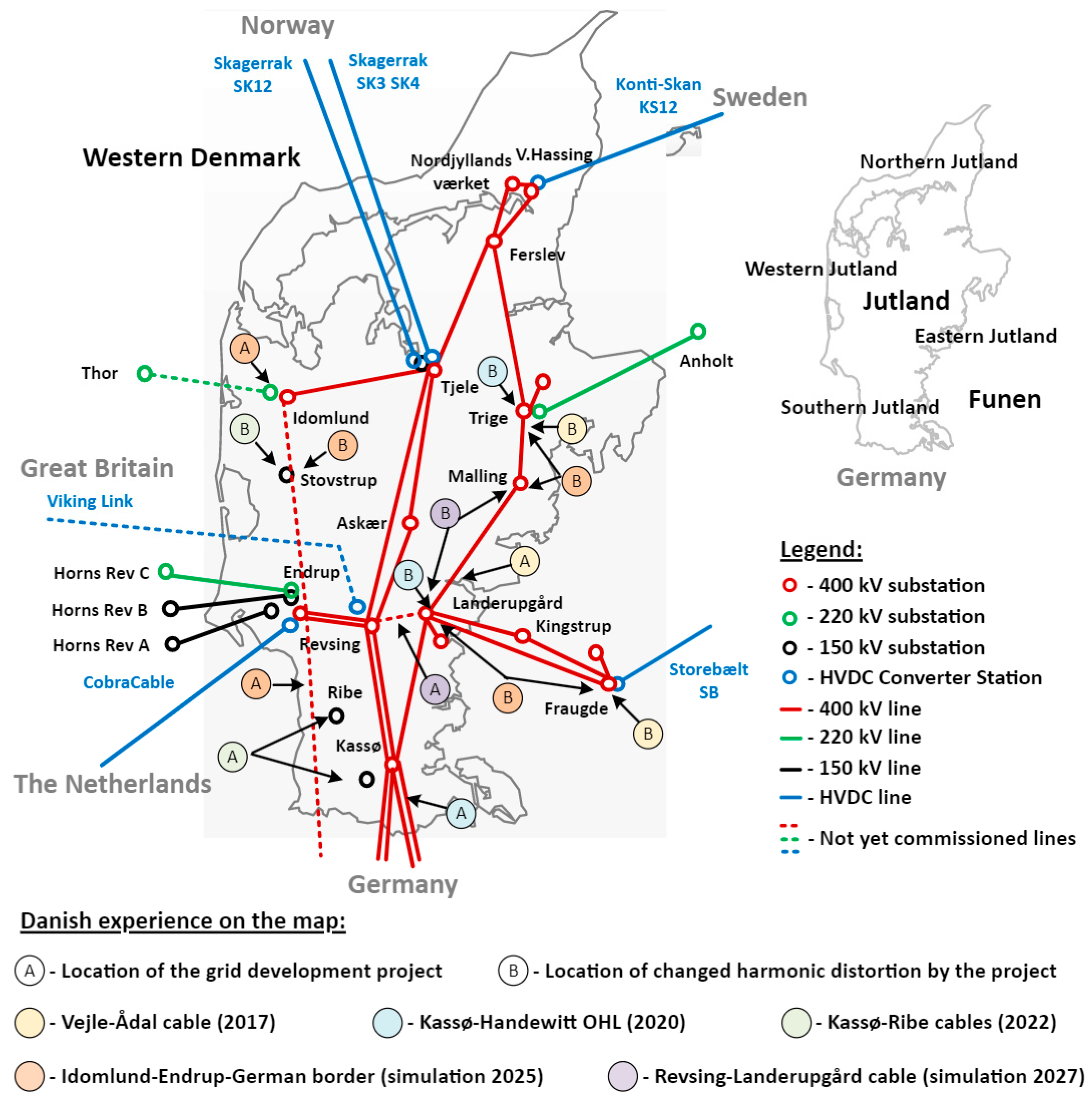
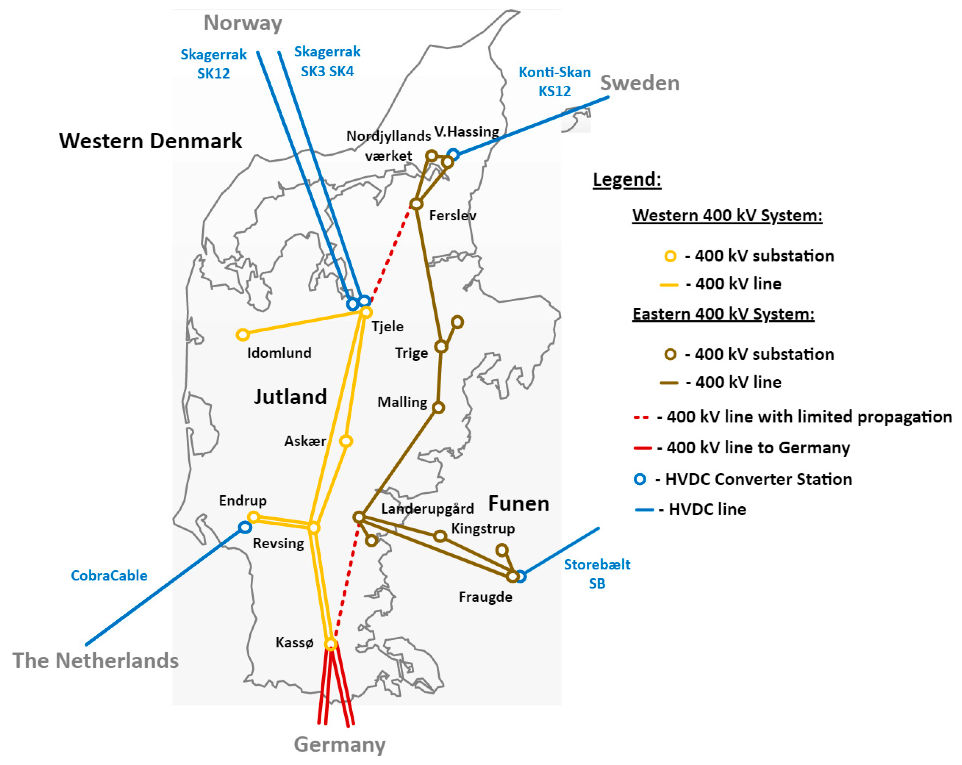
- The first is Eastern Denmark, which includes the main island of Zealand with the capital Copenhagen and the islands of Lolland, Falster, and Moen. The Eastern Danish transmission grid is HVAC-connected to Sweden and belongs to the Nordic synchronous system [15];
- The second is Western Denmark, which is HVAC-connected to Germany and belongs to the Continental European synchronous system.
2. Grid Development and Experience with Harmonic Distortion
- New 400 kV transmission lines must be established using UGCs to the extent that is technically feasible. Beyond what is technically feasible to establish using UGCs, OHLs must be used for 400 kV lines;
- Existing 132–150 kV OHLs are replaced with UGCs when the need for extensive reinvestment in the lines arises. Furthermore, existing 132–150 kV OHLs must be replaced with UGCs if the lines are in the vicinity of new 400 kV OHLs;
- New 132–150 kV transmission lines must be established using UGCs.
- The application of the 95th weekly percentiles of the ten-minute average harmonic voltage magnitudes when verifying the compliance of the measured harmonic distortion to the planning levels in [17];
- The application of the maxima of the three phase-to-ground harmonic voltage magnitudes, with reference to the nominal-frequency voltage, for comparison to the planning levels in [17].
3. Deterministic Method of Harmonic Distortion Simulation
3.1. Theoretical Background
- Validated data of the harmonic impedance of the HVDC Converter Stations as well as of the impedance of many distributed loads and generation units are not readily available [7].
- Specifically, the harmonic impedance of the LCC HVDC Converter Stations with nonlinear dependencies on both operation regime and control of the Converter Station itself and the operation regime of the grid is extremely difficult to obtain [7].
- The application of some kind of generic-level, not-validated data instead of unavailable vendor-specific or equipment-specific data would introduce another kind of inaccuracy to the simulation model. Such introduced inaccuracy would have unpredictable, uncontrollable influence on the results and shall hence be avoided.
- Their substations in the grid, denoted by the index N;
- The harmonic orders, denoted by the index k;
- The harmonic magnitudes and harmonic phase-angles;
- Asymmetry representing possible unbalance of the harmonic phase-current magnitudes.
3.2. Relative Components of Harmonic Source Vectors
3.3. Numerical Solution of Harmonic Source Vectors
- High magnitudes of the harmonic voltage distortion, i.e., those approaching and violating the planning levels, will be accurately simulated by the model;
- Low magnitudes, i.e., those significantly lower than the planning levels, will be accurately predicted as low but some larger relative discrepancy between the model and the harmonic voltage measurements can be accepted;
- The accuracy defined above shall be achieved for all harmonic orders included in the numerical tuning, all 400 kV substations of the Danish transmission grid, and all validation cases;
- High magnitudes imply the exceeding of 70% of the IEC planning level [17], the definition of which will be explained in Section 3.4.
- Vendor-specific sources;
- Distributed harmonic sources.
- Can be different for the different HVDC Converter Stations;
- Shall be the same for the different operation regimes of the same HVDC Converter Station.
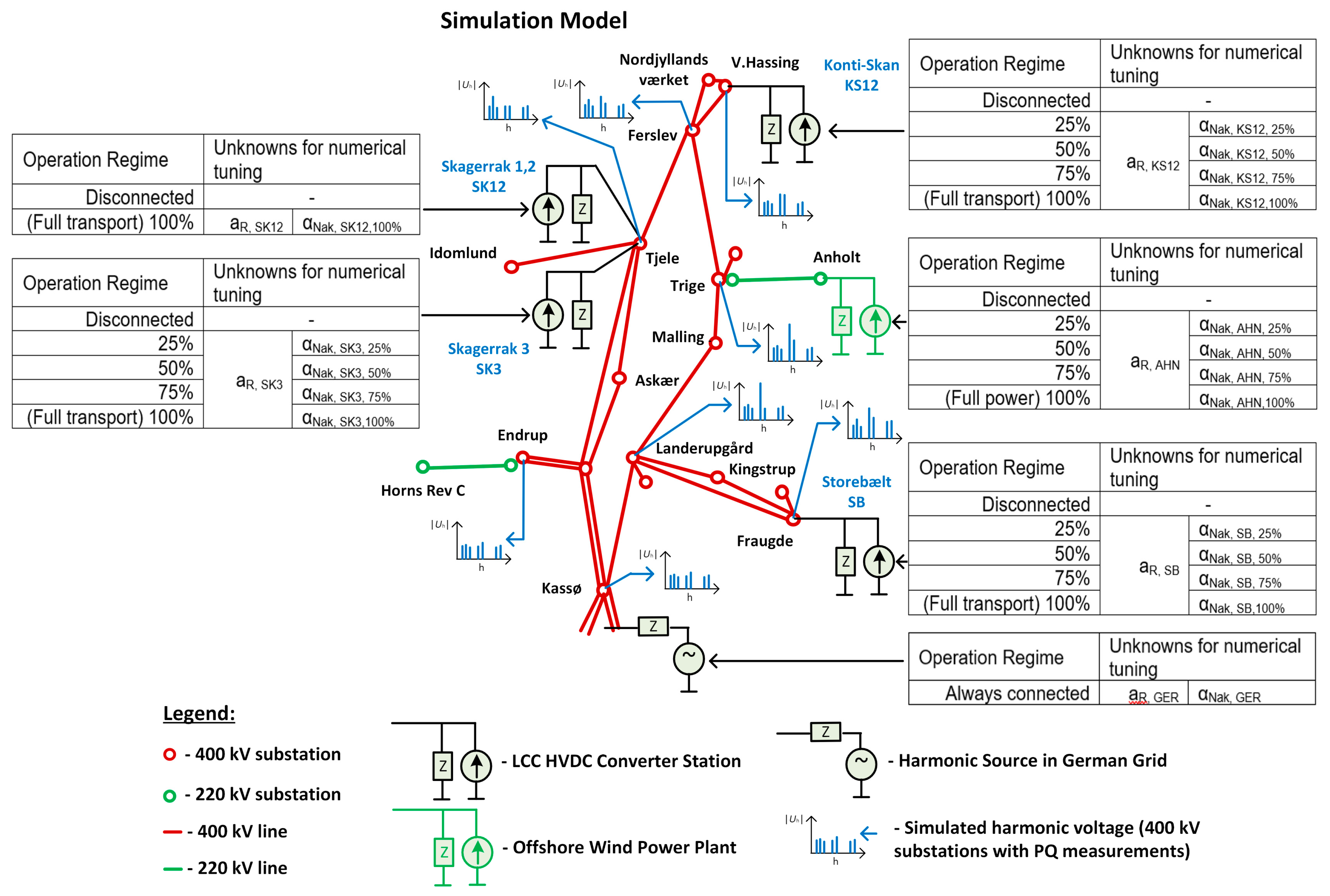
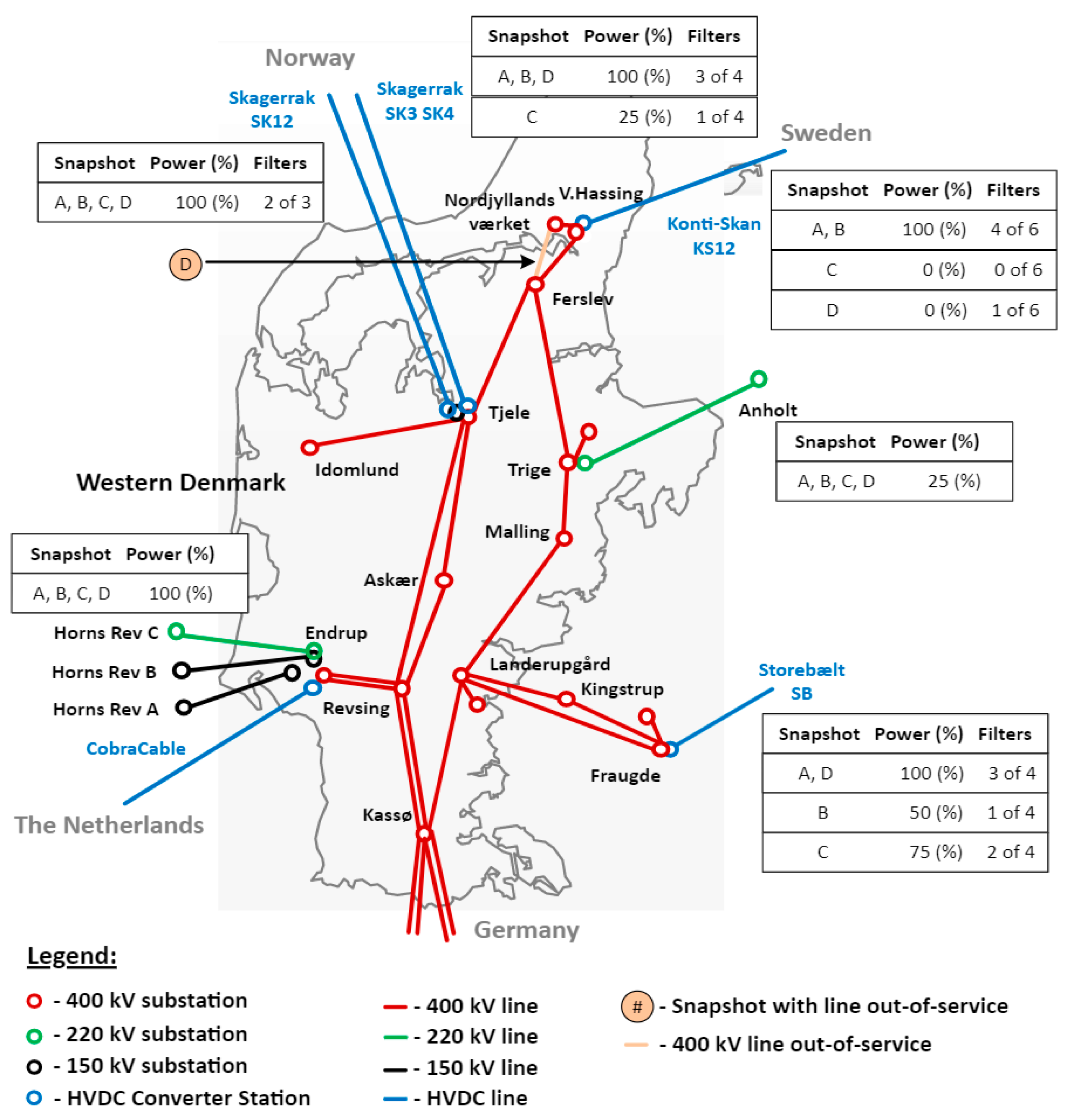
- The grid operation regimes (the passive part) and the operation regimes of the HVDC Converter Stations and Anholt OWPP are implemented in the simulation model of the Western Danish transmission grid.
- The AC load flow solutions are conducted for each operation regime.
- The parameters aR and αNak are assigned to the harmonic source models (HVDC, Anholt, and the harmonic voltage source in Germany) according to their operation regimes.
- The harmonic load flow solutions are conducted for each operation regime, and the maximum of the three line-to-ground harmonic voltage magnitudes are recorded for each harmonic order of the tuning and for each substation.
- The simulated harmonic voltage magnitudes are compared to the measured harmonic voltage magnitudes (maximum of the three line-to-ground harmonic voltages) for the 400 kV substations with available harmonic measurements.
- If the discrepancy is not acceptable, the parameters aR and αNak are adjusted and the procedure for solving the harmonic load flow and comparing the simulated and measured harmonic voltage magnitudes continues.
- When the discrepancy between the simulated and measured harmonic voltage magnitudes becomes small and acceptable, the tuning stops. The relative magnitudes and relative phase-angles for the representation of the harmonic emission from the HVDC and Anholt OWPP and the contribution of the German transmission grid in Denmark are fixed and locked.
3.4. Prediction of Harmonic Distortion following Grid Expansion
- Electro-geometrical and electrical data of new, not-yet-commissioned connections which are available at the time of the harmonic assessment may differ from the as-built data after commissioning;
- New harmonic emission sources with yet-unknown characteristics can be introduced in the transmission grid during or after the commissioning of the new connections;
- Initial inaccuracies in the numerical tuning of the relative magnitudes or relative phase-angles;
- Changes within foreign neighboring grids which are not properly addressed in the simulation model of the domestic transmission grid.
4. Simulation Model Development Process
5. Validation
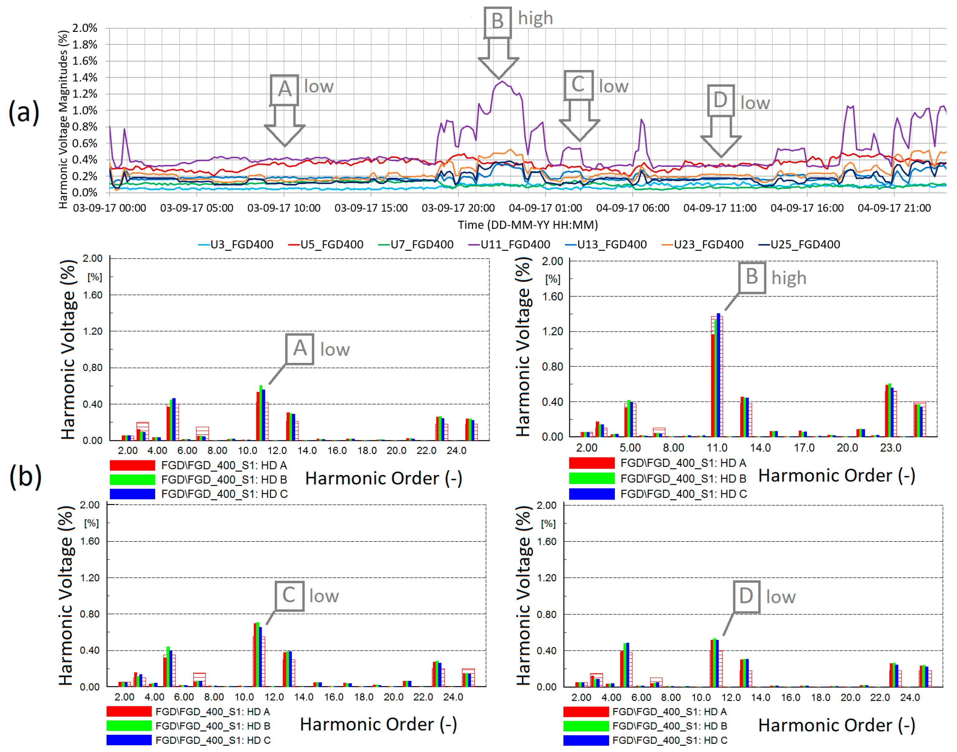
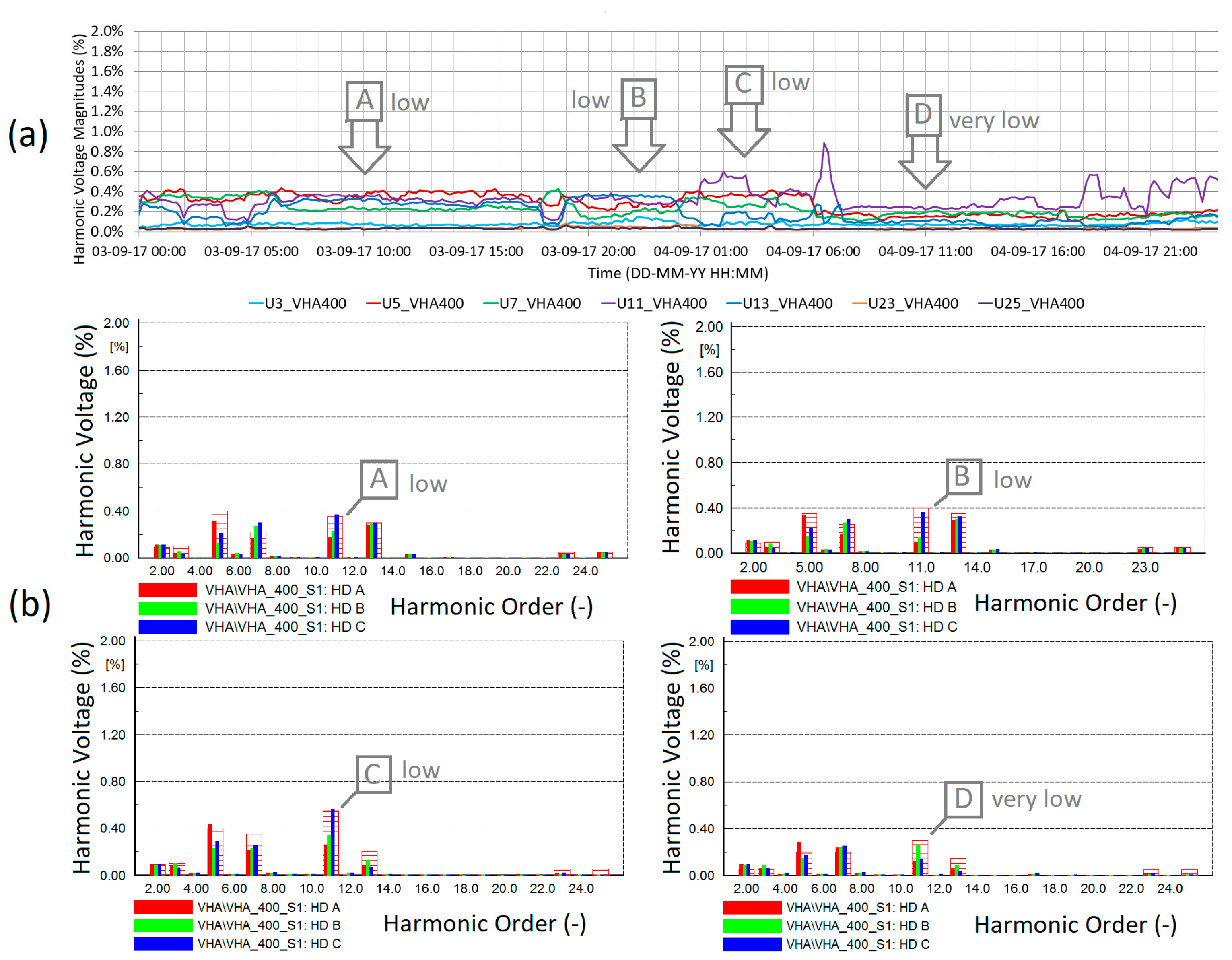
- solid red—simulated phase A;
- solid green—simulated phase B;
- solid blue—simulated phase C;
- shaded red background—measured maximum of the three phases for the grid stage after the energization of the Vejle-Ådal 400 kV UGC.
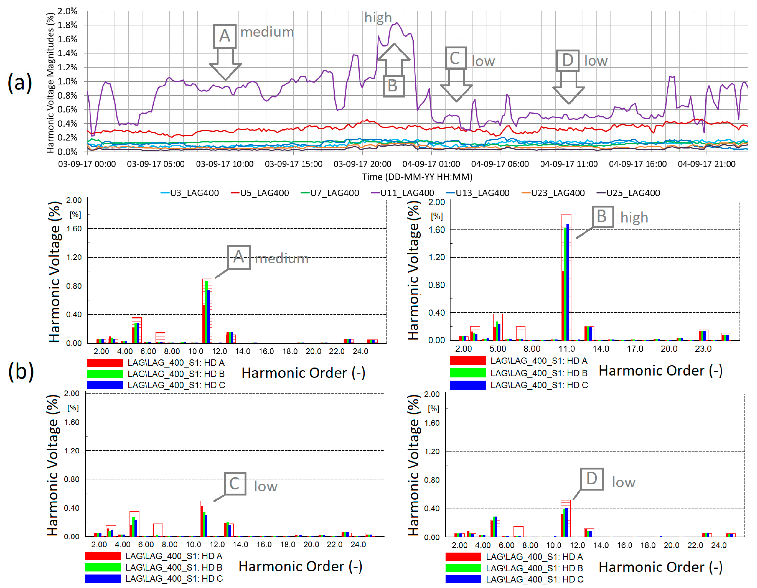
5.1. Period of Varying 11th Harmonic Distortion
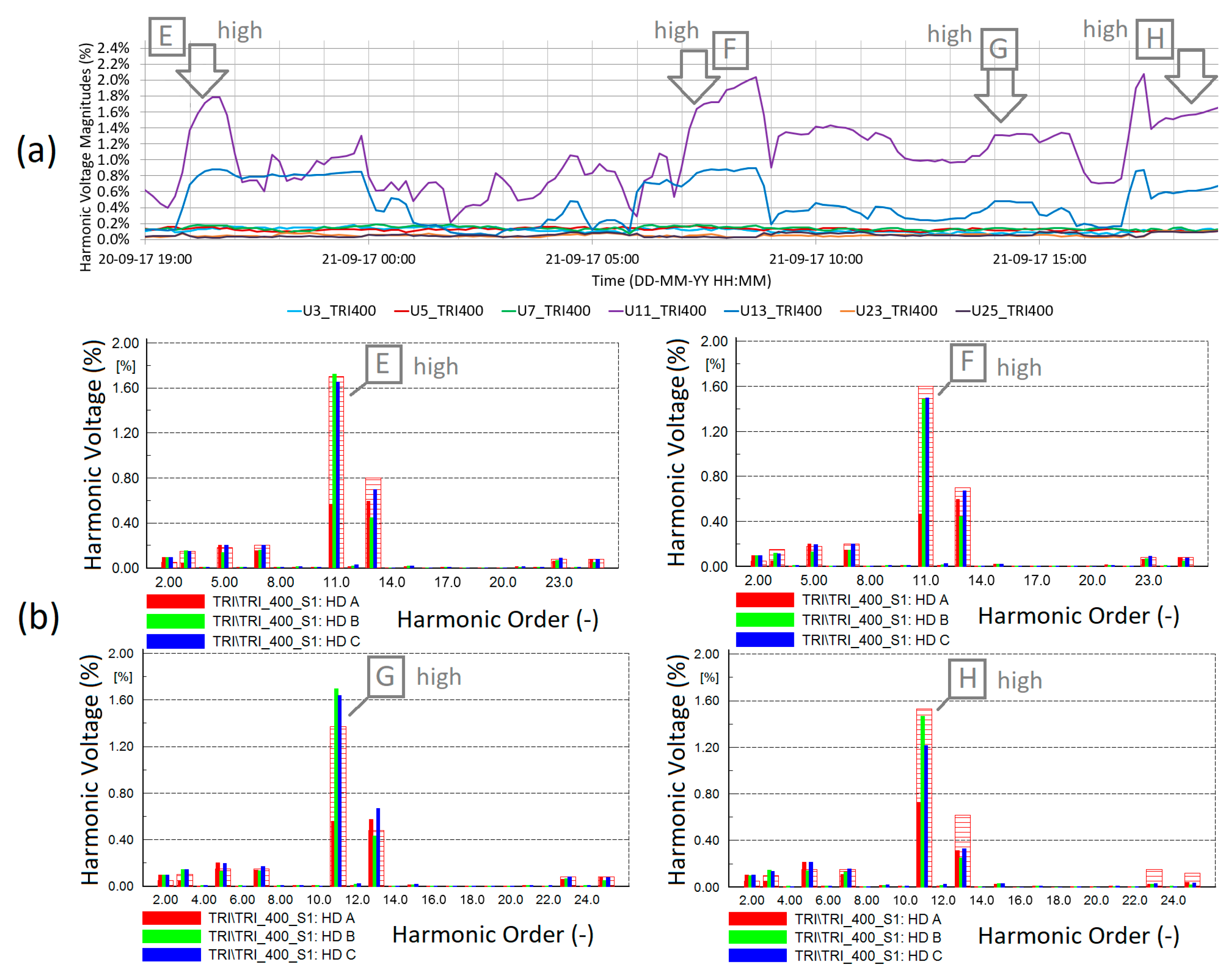
5.2. Period Containing High 11th Harmonic Voltage Magnitudes
5.3. Determining Harmonic Voltages of Not-Previously-Simulated Regimes
6. Prediction of Harmonic Voltage Distortion
- solid blue—simulated magnitudes for the grid stage before the Vejle-Ådal UGC;
- solid green—simulated magnitudes for the grid stage after the Vejle-Ådal UGC;
- red shaded—measured maximum for the grid stage after the Vejle-Ådal UGC.
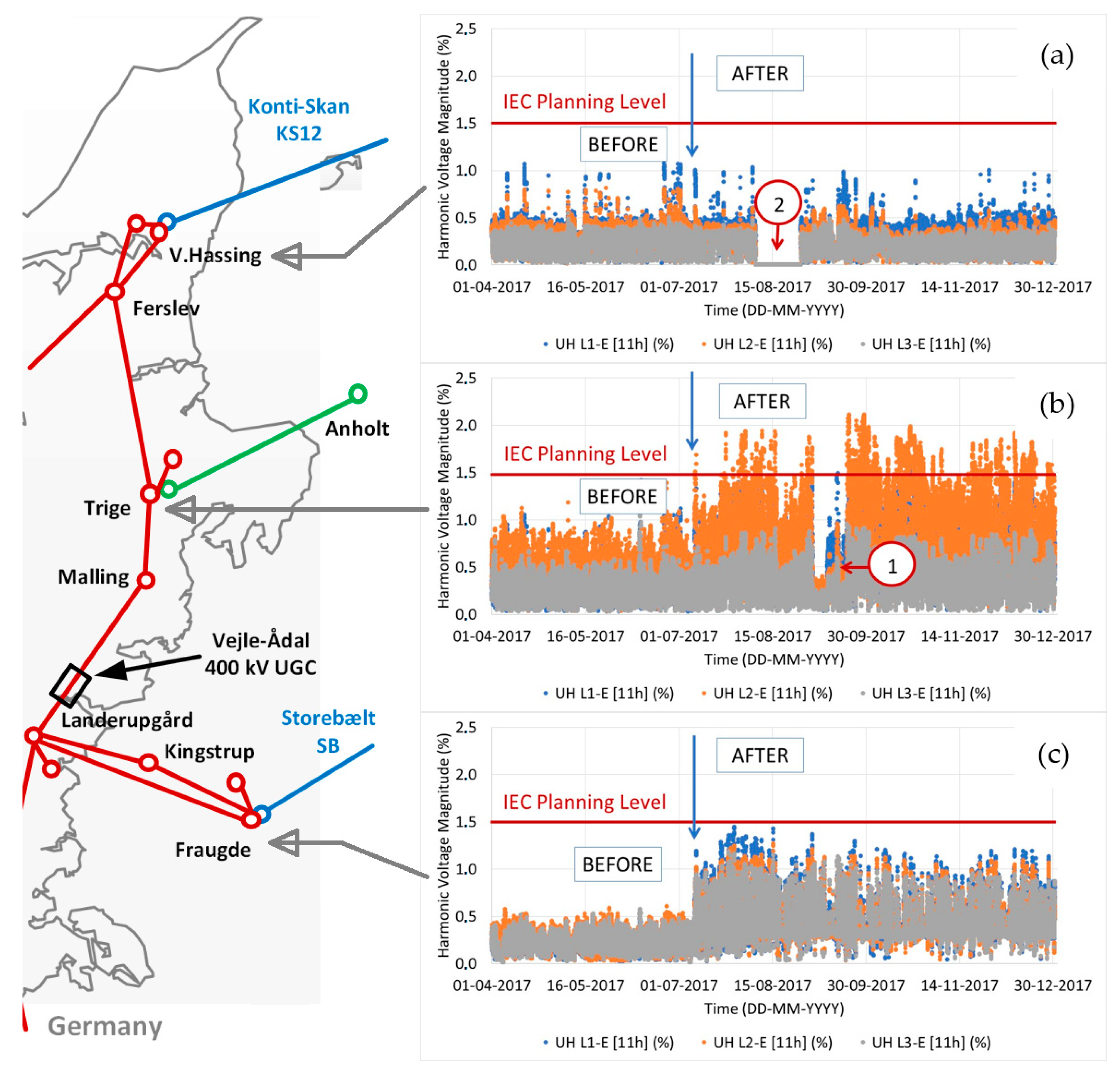
- Significantly changed harmonic voltage magnitudes in Trige and Fraugde;
- High and unchanged magnitudes in Landerupgård;
- Low and unchanged magnitudes in V. Hassing.
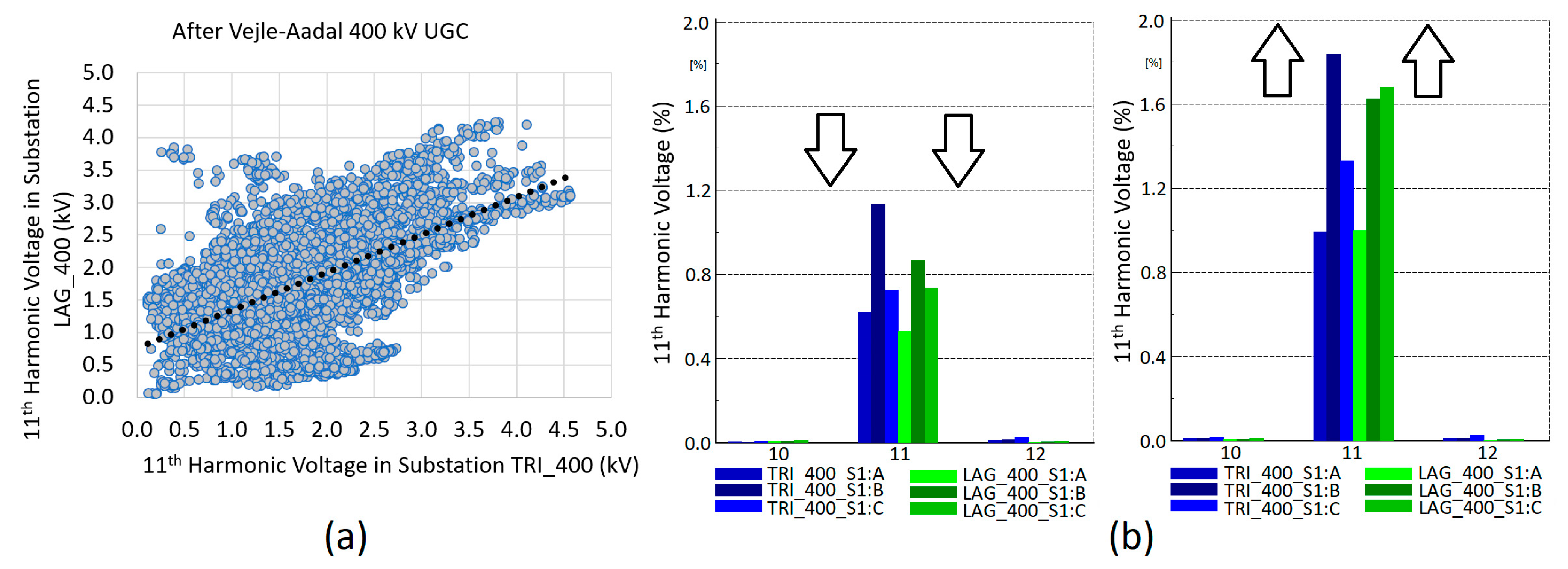
- In the present grid, there is a strong positive correlation between the 11th harmonic voltage magnitudes in Trige and Landerupgård, i.e., there are simultaneously increasing and decreasing magnitudes;
- In the grid before the energization of the Vejle-Ådal 400 kV UGC, there is a possibility of weak negative correlation. Negative correlation means increasing the 11th harmonic voltage magnitudes in one substation while decreasing them in the other substation in specific regimes. The correlation is pronounced weak due to the round shape of the measured dependency, as depicted in Figure 18a.
- The correlation patterns have not been conclusively demonstrated by observational analysis using the simulation model, but they will be examined in more detail in Section 8.
7. Accuracy of Deterministic Model
8. Analysis of Harmonic Patterns from Measurements
8.1. Preparing a Dataset
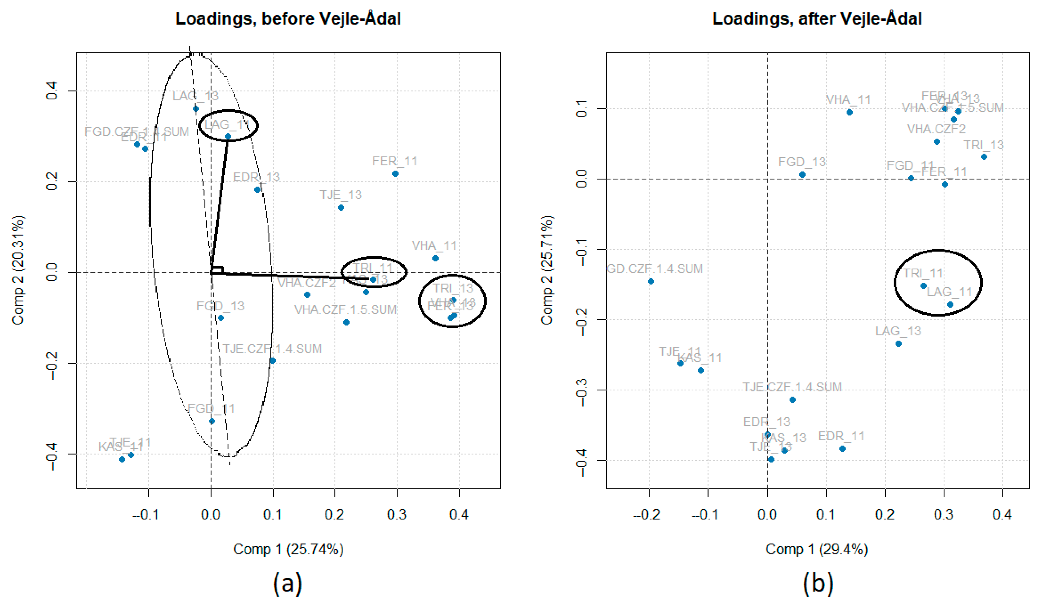
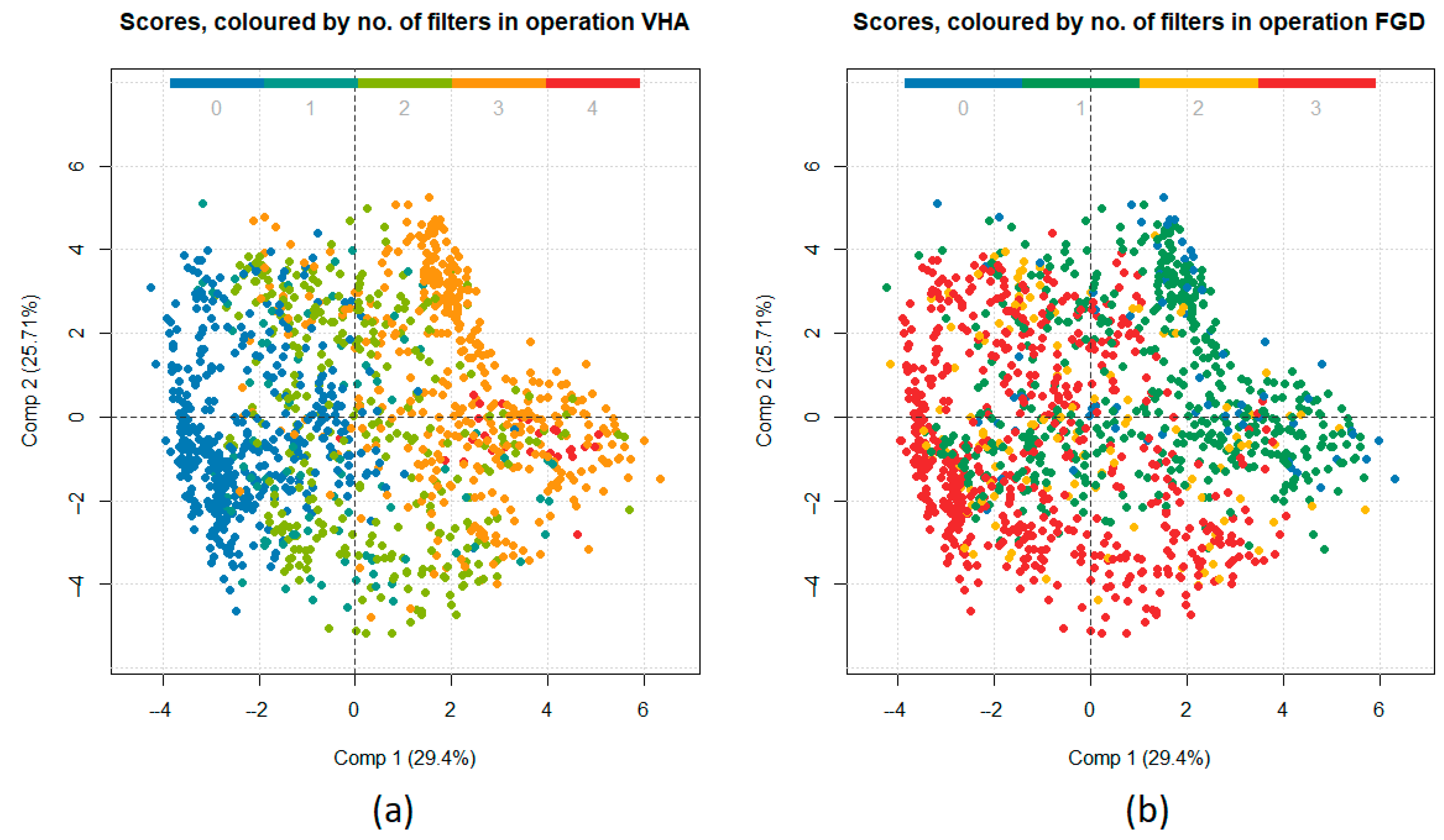
8.2. Principal Component Analysis
8.2.1. Before Vejle-Ådal
8.2.2. After Vejle-Ådal
9. Analysis of the Results Received
- Varying between low and high magnitudes of the 11th harmonic voltages, in the consecutive snapshots A through D as presented in Section 5.1;
- High magnitudes of the 11th harmonic voltages, as shown in the snapshots E through H in Section 5.2.
10. Conclusions
Author Contributions
Funding
Data Availability Statement
Conflicts of Interest
References
- Harmonic Study—Large Renewable Energy Generators; Australian Power Quality and Reliability Centre (APQRC): Fairy Meadow, Australia; University of Wollongong: Wollongong, Australia, 2022; 120p. Available online: https://arena.gov.au/assets/2022/05/harmonic-study-large-renewable-energy-generators-report.pdf. (accessed on 15 April 2023).
- Liyanage, S.; Perera, S.; Robinson, D. Harmonic Emission Assessment of Solar Farms: A Comparative Study Using EMT and Frequency Domain Models. CIGRÉ Sci. Eng. 2022, 1–21. [Google Scholar]
- Lange, A.G.; Redlarski, G. Selection of C-Type Filters for Reactive Power Compensation and Filtration of Higher Harmonics Injected into the Transmission System by Arc Furnaces. Energies 2020, 13, 2330. [Google Scholar] [CrossRef]
- Kazemi, R.; Lwin, M.; Leonard, J.; Fox, C.; Boessneck, E. Harmonic Modelling and Model Validation of DFIG Wind Turbines. Paper C4-301. In Proceedings of the CIGRÉ 2020 Session, Digital E-Session 2020, Paris, France, 24–28 August 2020. [Google Scholar]
- Guest, E.; Jensen, K.H.; Rasmussen, T.W. Sequence Domain Harmonic Modeling of Type IV Wind Turbines. IEEE Trans. Power Electron. 2018, 33, 4934–4943. [Google Scholar] [CrossRef]
- Technical Issues Related to New Transmission Lines in Denmark; Energinet: Erritsø, Denmark, 2018; 132p, Available online: https://energinet.dk/media/t2hnud0v/technical-issues-related-to-new-transmission-lines-in-denmark.pdf. (accessed on 15 April 2023).
- Network Modelling for Harmonic Studies; CIGRÉ, Join Working Group C4/B4.38; Technical Brochure 766; CIGRÉ: Paris, France, 2019; 241p.
- Final Report for Capital Project 966 Cable Integration Studies; PSC Reference: JI7867-03-02; Power Systems Consultants UK Ltd. for EirGrid PLC: Reading, UK, 2020; 168p, Available online: https://www.eirgridgroup.com/site-files/library/EirGrid/Cable-integration-studies-for-Kildare-Meath-Grid-Upgrade-Step-3.pdf (accessed on 24 April 2023).
- Schaefer, A.; Massat, S.; Hanson, J.; Balzer, G. Influence of Cabling on Harmonic Voltages in a Transmission Grid using an Exemplary Test Grid. Paper ID 11072. In Proceedings of the CIGRÉ 2022 Session, Paris, France, 28 August–2 September 2022; 12p. [Google Scholar]
- Lennerhag, O.; Rogersten, R.; Råström, S. A Parallel Resonance Investigation in Stockholm’s Future Cablified Transmission Grid: A Prospective Study on Transformer Energization. In Proceedings of the IEEE/PES Transmission and Distribution Conference and Exposition, Chicago, IL, USA, 12–15 October 2020. [Google Scholar]
- Power System Technical Performance Issues Related to the Application of Long HVAC Cables; CIGRÉ, Working Group C4.502; Technical Brochure 556; CIGRÉ: Paris, France, 2013; 124p.
- Jensen, C.F. Harmonic Background Amplification in Long Asymmetrical High Voltage Cable Systems. Electr. Power Syst. Res. 2018, 160, 292–299. [Google Scholar] [CrossRef]
- Kwon, J.B. System-wide Amplification of Background Harmonics due to the Integration of High Voltage Power Cables. Paper C4-305. In Proceedings of the CIGRÉ 2020 Session, Digital E-Session 2020, Paris, France, 24–28 August 2020. [Google Scholar]
- Akhmatov, V.; Hansen, C.S.; Jakobsen, T. Development of a Harmonic Analysis Model for a Meshed Transmission Grid with Multiple Harmonic Emission Sources. Paper WIW20-39. In Proceedings of the 19th Wind Integration Workshop 2020—International Workshop on Large-Scale Integration of Wind Power into Power Systems as well as on Transmission Networks for Offshore Wind Power Plants, Virtual, 11–12 November 2020. [Google Scholar]
- Akhmatov, V.; Sørensen, M.; Jakobsen, T.; Skovgaard, C.L.; Gellert, B.C.; Bukh, B.S. Harmonic Distortion Prediction Method for a Meshed Transmission Grid with Distributed Harmonic Emission Sources—Eastern Danish Transmission Grid Case Study. Paper WIW22-04. In Proceedings of the 21st Wind & Solar Integration Workshop, The Hague, The Netherlands, 12–14 October 2022. [Google Scholar]
- Bukh, B.S.; Bak, C.L.; Da Silva, F.F. Analysis of Harmonic Propagation in Meshed Power Systems Using Standing Waves. Paper C4-563. In Proceedings of the CIGRÉ 2022 Session, Paris, France, 28 August—2 September 2022. [Google Scholar]
- IEC 61000-3-6; Electromagnetic Compatibility (EMC)—Part 3–6: Limits—Assessment of Emission Limits for the Connection of Distorting Installations to MV, HV and EHV power systems. International Electrotechnical Commission: Geneva, Switzerland, 2016; 58p.
- Demand Connection Code. Commission Regulation (EU) 2016/1388, ENTSO-E, 17 August 2016. Available online: https://www.entsoe.eu/network_codes/dcc/ (accessed on 24 April 2023).
- Requirements for Generators. Commission Regulation (EU) 2016/631, ENTSO-E, 14 April 2016. Available online: https://www.entsoe.eu/network_codes/rfg/ (accessed on 24 April 2023).
- Lennerhag, O.; Bollen, M.H.J. A Stochastic Aggregate Harmonic Load Model. IEEE Trans. Power Deliv. 2020, 35, 2127–2135. [Google Scholar] [CrossRef]
- Arrilaga, J.; Watson, N.R. Harmonic sources. In Power System Harmonics, 2nd ed.; John Wiley & Sons, Ltd.: Chichester, UK, 2003; Chapter 3; pp. 61–142. [Google Scholar]
- Abdi, H.; Williams, L.J. Principal Component Analysis. Wiley Interdiscip. Reviews. Comput. Stat. 2010, 2, 433–459. [Google Scholar] [CrossRef]
- Bro, R.; Smilde, A.K. Principal Component Analysis. Anal. Methods 2014, 6, 2812–2831. [Google Scholar] [CrossRef]
- Sanguansat, P. Principal Component Analysis: Engineering Applications; IntechOpen: Rijeka, Croatia, 2012; ISBN 953-51-5693-4. [Google Scholar]


| Unit | Substation | Main Harmonic Orders |
|---|---|---|
| Konti-Skan 1, 2 (740 MW) 1 | V. Hassing 400 kV | 11, 13, 23, 25 |
| Skagerrak 3 (500 MW) 1 | Tjele 400 kV | 11, 13, 23, 25 |
| Skagerrak 1, 2 (550 MW) 1 | Tjele 150 kV | 11, 13, 23, 25 |
| Storebælt (600 MW) 1 | Fraugde 400 kV | 11, 13, 23, 25 |
| Anholt (400 MW) 2 | Anholt 220 kV 3 | 11, 13 |
| Horns Rev C (400 MW) 2 | Horns Rev C 220 kV 3 | 11, 13 4 |
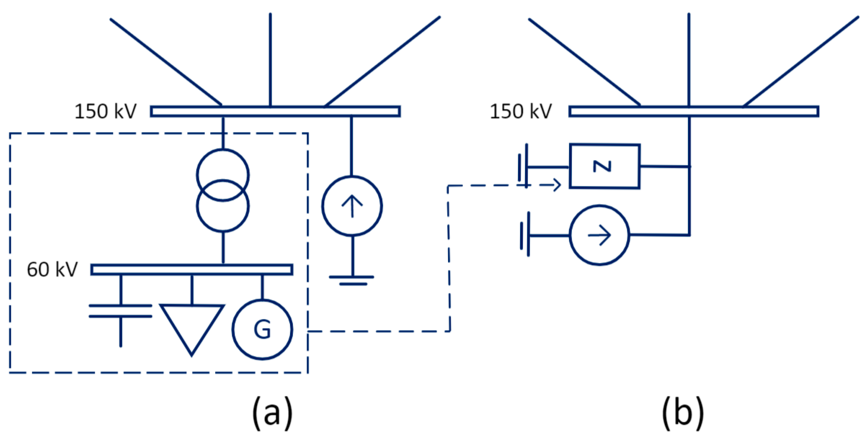
| Distributed sources | 150 kV substations | 2, 3, 5, 7 |
| Variable | Description |
|---|---|
| xxx_11 (kV) | Measured 11th harmonic voltage; xxx indicates substation with measurement |
| xxx_13 (kV) | Measured 13th harmonic voltage; xxx indicates substation with measurement |
| VHA. CZF.1.5.SUM | Number of harmonic filters in operation at substation V. Hassing 400 kV (VHA) with HVDC system KS12 |
| VHA. CZF2 | AC filter (of other type) in operation at substation VHA |
| FGD. CZF.1.4.SUM | Number of harmonic filters in operation at substation Fraugde 400 kV (FGD) with HVDC system SB |
| I. CZF.1.4.SUM | Number of harmonic filters in operation at substation Tjele 400 kV (I) with HVDC system SK3 |
Disclaimer/Publisher’s Note: The statements, opinions and data contained in all publications are solely those of the individual author(s) and contributor(s) and not of MDPI and/or the editor(s). MDPI and/or the editor(s) disclaim responsibility for any injury to people or property resulting from any ideas, methods, instructions or products referred to in the content. |
© 2023 by the authors. Licensee MDPI, Basel, Switzerland. This article is an open access article distributed under the terms and conditions of the Creative Commons Attribution (CC BY) license (https://creativecommons.org/licenses/by/4.0/).
Share and Cite
Akhmatov, V.; Søndergaard Bukh, B.; Liberty Skovgaard, C.; Gellert, B.C. Novel Harmonic Distortion Prediction Methods for Meshed Transmission Grids with Large Amount of Underground Cables. Energies 2023, 16, 3965. https://doi.org/10.3390/en16093965
Akhmatov V, Søndergaard Bukh B, Liberty Skovgaard C, Gellert BC. Novel Harmonic Distortion Prediction Methods for Meshed Transmission Grids with Large Amount of Underground Cables. Energies. 2023; 16(9):3965. https://doi.org/10.3390/en16093965
Chicago/Turabian StyleAkhmatov, Vladislav, Bjarne Søndergaard Bukh, Chris Liberty Skovgaard, and Bjarne Christian Gellert. 2023. "Novel Harmonic Distortion Prediction Methods for Meshed Transmission Grids with Large Amount of Underground Cables" Energies 16, no. 9: 3965. https://doi.org/10.3390/en16093965