
Optimal Placement of Battery Swapping Stations for Power Quality Improvement: A Novel Multi Techno-Economic Objective Function Approach


Abstract
:1. Introduction
1.1. Importance and Motivations
1.2. Literature Review
1.3. Contributions
- Suggesting an innovative mixed multi-objective framework for resolving optimal placement challenges, this framework relies on the combination of elitist non-dominated sorting and the crowding distance mechanism. The multi-objective approach introduced can handle numerous and contradictory objectives during the process of optimizing problems. Its formulation employs the principles of elitist, non-dominated sorting and the crowding distance mechanism. Moreover, this approach effectively addresses unconstrained, constrained, and engineering design problems, encompassing a wide range of linear, nonlinear, continuous, and discrete characteristics that define Pareto front problems.
- This study aims to determine the optimal location for BSSs in a distribution network, considering both technical and economic factors. This study differs from the previous research by incorporating a comprehensive framework that considers multiple objectives, such as network reliability and power quality. The approach involves strategically placing BSSs based on their quantity, positioning, and capacity while also considering technical metrics associated with MG, such as preventing alterations in short-circuit levels to maintain protective configurations.
- Incorporating reliability measures such as the anticipated energy shortage (EENS) and voltage sensitivity indices of the system, alongside economic aims.
- Accounting for power quality aspects of the network, such as voltage deviations, losses, and loss sensitivity indices, within the context of an optimal placement problem.
1.4. Organization
2. Conceptual Framework
- Proposing a groundbreaking mixed multi-objective framework to address the challenges of optimal placement. This framework combines elitist non-dominated sorting with the crowding distance mechanism.The multi-objective approach introduced is capable of handling multiple and often conflicting objectives during the optimization process. Its formulation incorporates the principles of elitist, non-dominated sorting and the crowding distance mechanism. Furthermore, this approach effectively addresses a wide range of problems, including unconstrained, constrained, and engineering design problems, encompassing various linear, nonlinear, continuous, and discrete characteristics that define Pareto front problems.
- Considering technical metrics related to MGs, such as maintaining protective configurations by preventing changes in short-circuit levels, alongside economic objectives when determining the best placement for BESS units.
- Incorporating reliability measures, including the anticipated energy shortage (EENS) and voltage sensitivity indices of the system, in addition to economic goals.
- Accounting for power quality aspects of the network, including voltage deviations, losses, and loss sensitivity indices, as part of the optimal placement problem.
3. Mathematical Problem Formulations
- The initial data of the power network, including factors such as the load profile, DG units generation, electricity pricing, and the initial configuration of the power network under normal operating conditions, are retrieved by the central processing system.
- In the subsequent stage, the power flow analysis is conducted, taking into account the initial techno-economic indices of the power system.
- Following the power flow analysis, the proposed multi-objective framework is invoked. Its purpose is to determine the optimal quantity, ideal locations, and appropriate sizes for the BSS units, ultimately optimizing the objective function. This objective function encompasses various techno-economic indices of the power system and is compared against the initial normal operation of the power system. These steps collectively form the core of our proposed approach for optimizing the placement of BSSs within distribution networks, contributing to improved energy management, enhanced technical performance, and increased system reliability.
3.1. Cost Modeling of Distributed Generation Units (PV and Wind Generation)
3.2. Cost Modeling of the Traditional Generation Units
- : Penalty factor for CO2 production.
- : Penalty factor for SO2 production.
- : Penalty factor for NOx production.
3.3. Battery Swapping Station Modeling
3.4. Power Losses and Loss Sensitivity Factor
3.5. Voltage Deviations Formulations
3.6. Short Circuit Level Criteria Modeling
3.7. Voltage Sensitivity Index
3.8. Expected Energy Not Served (EENS) Criteria
3.9. Objective Function Formulation
4. Multi-Objective Optimization Method
5. Simulation Results and Discussion
5.1. Input Parameters of the System
5.2. Results Analysis
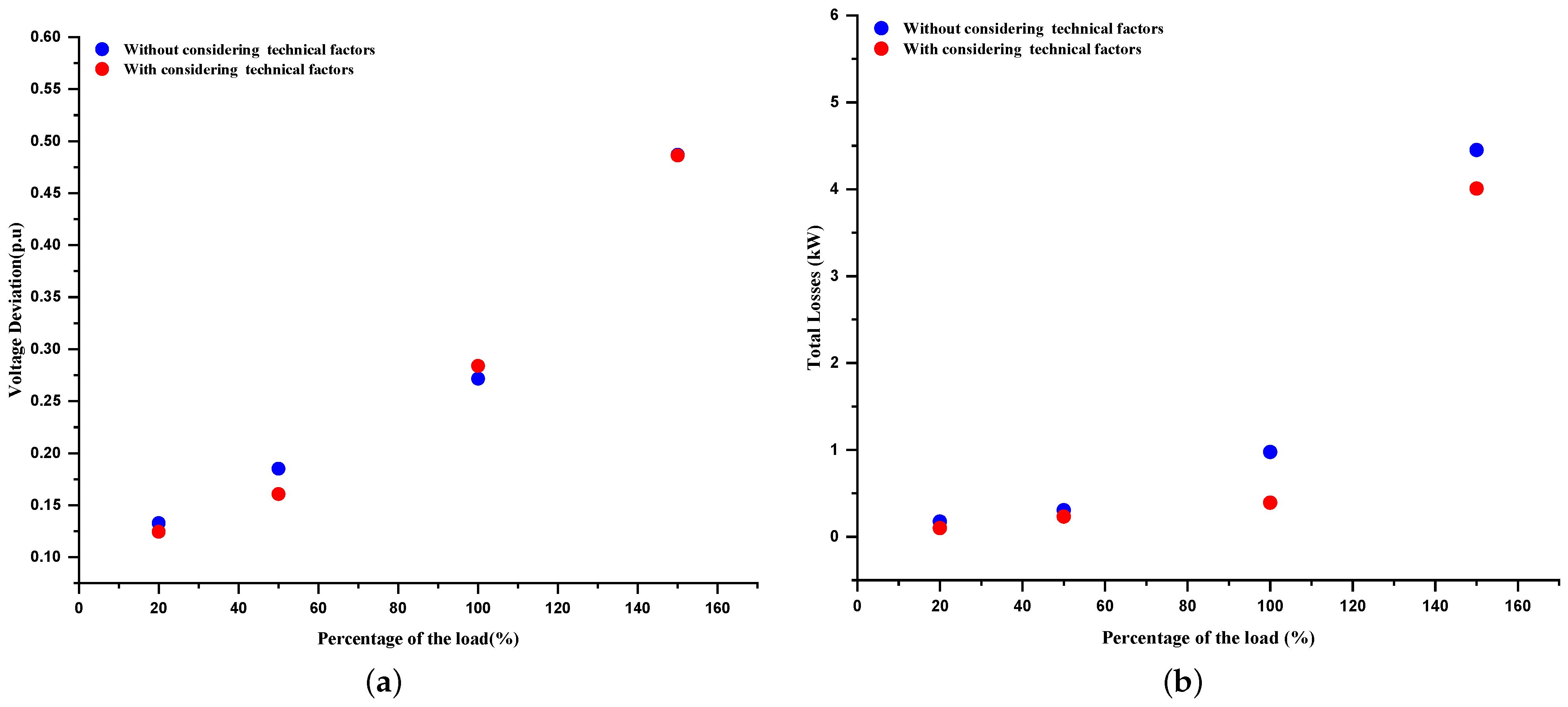
- In Figure 16a,b, it is evident that during most hours of the day, the voltage deviation and network loss graphs displayed lower values when the BSSs were optimally placed within the power network. However, when considering the presence of optimally located BSSs, additional factors such as reliability and short-circuit levels were also taken into consideration, introducing extra constraints in the quest for the best solution. Conversely, as indicated by Figure 16a, there was only an increase in voltage deviation during the states of more than 50% of the nominal load, compared to scenarios where the technical factor capability was not factored in. This increase was a result of improvements in other economic and security indicators within the network, contributing to the overall optimal solutions. Additionally, during these hours, as illustrated in Figure 12, the BSSs adjusted their charge states to redirect power flow in a manner that optimized all objective functions indicators. Moreover, according to Table 3, Table 4 and Table 5, the summation of the total losses from 20% to 150% of the nominal load is less than the states without considering the technical factors.
- Figure 16c and the results of Table 3, Table 4 and Table 5 show the operating cost of the system in the state of the optimal placement of batteries by considering that the technical parameters of the network in most cases of load changes are slightly higher than the case of not considering the technical parameters of the network in some cases, like in 20% of freight where the operating cost is also lower. This is while the technical parameters of the network are in a more favorable condition in all cases.
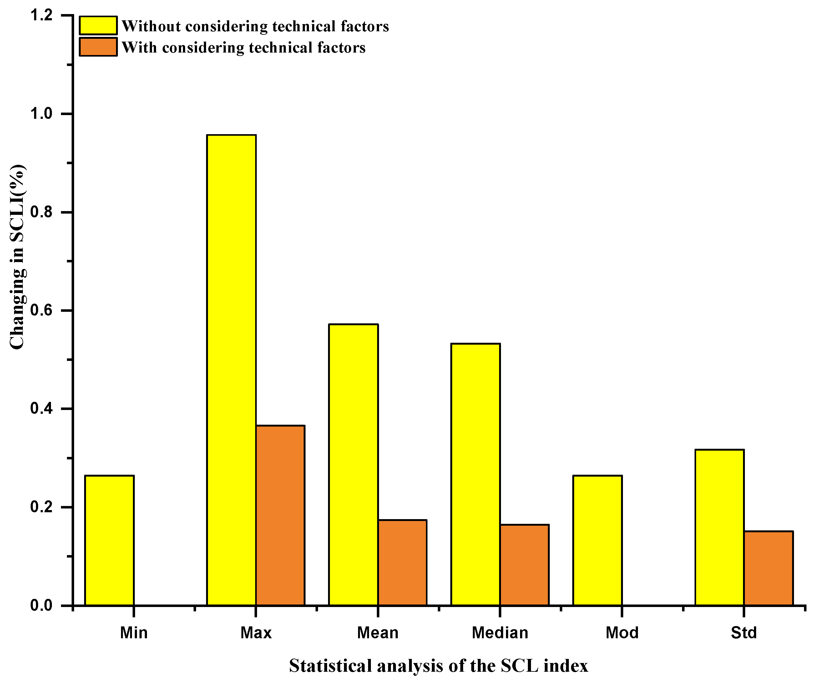
- As previously mentioned, one of the pivotal indicators to be taken into account when optimizing the placement of BSSs in power distribution networks is the short-circuit level variation index. This index holds immense importance as alterations in the short-circuit level, stemming from changes in production and network topology, have the potential to disrupt the protective system configurations, resulting in substantial damages and costs to the system. Consequently, as depicted in Figure 16d, the short-circuit level variation index approaches less than 0.5 when it is considered in the optimal placement of BSSs within the network. This capability plays a crucial role in averting disruptions to the protective system configurations through the optimal charging and discharging of BSSs during the operation of the power network.
- Through an analysis of Figure 16e, it becomes evident that the network’s reliability status, as assessed by the total energy not supplied to the network indicator, exhibits notably reduced values in all states of changing load (20% to 150%). Nevertheless, when looking at Table 3, Table 4 and Table 5 in a broader context, it can be concluded that the utilization of the reliability indices (EENS index) in optimal placement of BSSs in the network and control of the states of charge/discharge for BSSs within the network results in substantially lower total energy supplied to the entire system, in sharp contrast to scenarios where the capability of reliability is not taken into consideration.
- The problem of optimal placement of BSSs is a complex one that involves various objectives and constraints. To make informed decisions, it is crucial to prioritize these objectives and constraints effectively. Here are some key considerations:
- Coverage and Quality of Technical Service (QoS)Prioritize ensuring comprehensive coverage of the MG area to provide reliable services to all consumers. QoS parameters, such as voltage sensitivity, voltage deviations, short circuit level, losses, and loss sensitivity factor, should be prioritized to meet the specific consumers’ needs of different applications within the MG.
- CostCost considerations are essential, as deploying BSSs can be expensive. Prioritize minimizing the deployment and operational costs, which may include equipment costs, power consumption, maintenance expenses, and backhaul connectivity costs.
- Energy EfficiencyIn MGs, energy conservation is critical. Therefore, it is necessary to prioritize the deployment of BSSs in a way that minimizes their energy consumption, as excessive power usage can strain the microgrid’s resources.
- Reliability and RedundancyPrioritize ensuring high reliability and redundancy in supply energy to consumers. Redundant BSSs placement can be prioritized to ensure backup connectivity in case of failures.
- Environmental ImpactGiven the increasing focus on sustainability, prioritize solutions that minimize the environmental impact of BSSs deployment, such as reducing carbon emissions or avoiding disruption to local ecosystems.
- Voltage SecurityPrioritize the security concerns, such as VSI within the MG. Secure BSSs placement can help reduce vulnerabilities.
6. Conclusions

| Bus Number | Optimal State of ch/discharge (kWh) of BSSs at Different Percentages of Nominal Load | Bus Number | Optimal State of ch/discharge (kWh) of BSSs at Different Percentages of Nominal Load | ||||||
|---|---|---|---|---|---|---|---|---|---|
| 20% | 50% | 100% | 150% | 20% | 50% | 100% | 150% | ||
| 1 | 138.56 | 0.00 | 0.00 | −197.20 | 60 | 0.00 | 239.05 | −250.00 | −250.00 |
| 2 | −250.00 | 157.67 | 0.00 | −15.82 | 61 | 0.00 | 0.00 | 0.00 | 250.00 |
| 3 | 0.00 | 0.00 | 250.00 | 250.00 | 62 | 0.00 | 0.00 | −250.00 | −250.00 |
| 4 | 0.00 | 0.00 | −250.00 | 0.00 | 63 | 0.00 | −191.86 | 0.00 | 222.32 |
| 5 | 250.00 | 0.00 | −250.00 | 0.00 | 64 | 0.00 | 182.76 | −250.00 | −190.80 |
| 6 | −250.00 | 111.11 | −250.00 | 0.00 | 65 | 0.00 | 183.32 | −250.00 | 250.00 |
| 7 | 0.00 | 0.00 | −250.00 | 0.00 | 66 | 113.71 | 0.00 | 0.00 | −55.50 |
| 8 | 87.61 | −34.94 | 0.00 | 250.00 | 67 | 250.00 | 0.00 | 0.00 | 0.00 |
| 9 | 0.00 | −250.00 | −250.00 | 0.00 | 68 | 60.14 | 0.00 | 0.00 | 72.03 |
| 10 | 7.31 | −197.36 | 0.00 | 0.00 | 69 | −193.79 | 58.49 | 0.00 | 0.00 |
| 11 | 0.00 | −11.42 | 0.00 | 0.00 | 70 | 0.00 | 0.00 | −250.00 | −177.43 |
| 12 | −236.30 | −236.46 | 0.00 | −81.55 | 71 | 0.00 | 166.56 | 0.00 | −250.00 |
| 13 | 0.00 | 211.92 | 0.00 | 0.00 | 72 | 0.00 | 250.00 | 0.00 | −169.07 |
| 14 | −250.00 | 111.12 | 0.00 | 250.00 | 73 | 0.00 | −148.41 | 250.00 | 0.00 |
| 15 | 0.00 | −136.37 | 0.00 | 0.00 | 74 | 84.17 | 0.00 | −250.00 | 250.00 |
| 16 | 250.00 | −240.31 | 0.00 | 0.00 | 75 | 0.00 | 207.96 | −250.00 | 0.00 |
| 17 | 190.02 | −92.16 | −250.00 | 0.00 | 76 | 0.00 | 77.16 | 0.00 | −214.39 |
| 18 | 0.00 | 0.00 | 0.00 | −183.53 | 77 | 250.00 | 0.00 | 0.00 | −250.00 |
| 19 | 0.00 | 0.00 | 250.00 | 0.00 | 78 | 0.00 | −250.00 | 0.00 | 0.00 |
| 20 | −140.01 | 0.00 | 0.00 | −39.10 | 79 | 250.00 | −250.00 | −250.00 | 49.23 |
| 21 | −250.00 | −213.98 | −250.00 | 202.38 | 80 | 0.00 | 0.00 | 0.00 | 0.00 |
| 22 | 0.00 | −52.04 | −250.00 | 250.00 | 81 | 0.00 | 0.00 | 0.00 | 0.00 |
| 23 | 250.00 | 101.51 | 0.00 | 118.48 | 82 | 0.00 | −76.59 | 0.00 | −250.00 |
| 24 | 0.00 | −250.00 | 0.00 | 0.00 | 83 | 178.44 | 250.00 | −250.00 | −250.00 |
| 25 | 0.00 | 0.00 | 0.00 | 0.00 | 84 | 0.00 | −0.26 | 0.00 | 0.00 |
| 26 | 0.00 | 250.00 | 0.00 | 0.00 | 85 | 0.00 | 0.00 | 0.00 | 0.00 |
| 27 | 184.44 | −250.00 | 0.00 | 0.00 | 86 | 0.00 | 0.00 | 0.00 | −187.20 |
| 28 | 0.00 | −250.00 | 0.00 | −135.23 | 87 | 0.00 | −222.40 | 0.00 | 0.00 |
| 29 | −242.27 | 140.61 | −250.00 | 0.00 | 88 | 236.89 | 28.63 | −250.00 | −250.00 |
| 30 | 0.00 | −32.37 | −250.00 | 0.00 | 89 | 0.00 | −83.06 | 0.00 | −166.05 |
| 31 | 0.00 | −250.00 | 0.00 | 0.00 | 90 | −239.91 | 139.69 | −250.00 | 49.34 |
| 32 | −88.75 | 0.00 | 0.00 | −67.77 | 91 | 0.00 | 0.00 | 0.00 | −250.00 |
| 33 | 0.00 | −250.00 | −250.00 | 0.00 | 92 | 0.00 | 230.36 | 0.00 | 0.00 |
| 34 | 250.00 | 0.00 | 0.00 | 0.00 | 93 | −121.41 | −248.28 | −250.00 | 0.00 |
| 35 | 0.00 | 0.00 | −250.00 | 0.00 | 94 | −250.00 | 0.00 | 0.00 | 250.00 |
| 36 | 0.00 | −250.00 | 0.00 | −55.74 | 95 | 250.00 | 167.54 | 250.00 | 0.00 |
| 37 | 0.00 | −190.92 | 0.00 | 0.00 | 96 | 0.00 | 0.00 | 0.00 | 246.84 |
| 38 | −182.08 | 0.00 | 0.00 | 0.00 | 97 | −27.63 | 78.52 | −248.75 | 0.00 |
| 39 | 0.00 | 185.55 | 0.00 | 0.00 | 98 | −43.60 | 0.00 | 0.00 | 0.00 |
| 40 | 0.00 | 223.58 | −250.00 | 145.84 | 99 | 181.41 | 250.00 | 0.00 | 0.00 |
| 41 | 0.00 | −250.00 | −250.00 | 0.00 | 100 | −85.70 | 0.00 | 0.00 | 213.07 |
| 42 | 0.00 | −232.40 | 0.00 | 0.00 | 101 | 0.00 | 0.00 | 0.00 | 0.00 |
| 43 | 0.00 | 0.00 | 0.00 | −223.53 | 102 | 0.00 | 0.00 | 0.00 | 0.00 |
| 44 | 10.31 | 85.34 | 0.00 | 0.00 | 103 | 0.00 | −122.32 | 250.00 | 0.00 |
| 45 | 0.00 | 0.00 | 0.00 | 0.00 | 104 | 126.18 | −250.00 | −250.00 | 142.39 |
| 46 | 0.00 | 174.10 | 0.00 | 0.00 | 105 | 0.00 | 223.13 | 0.00 | −250.00 |
| 47 | 0.00 | 48.79 | −250.00 | 0.00 | 106 | −240.53 | −92.01 | 0.00 | 87.27 |
| 48 | 0.00 | −61.71 | −245.94 | −34.96 | 107 | −250.00 | 0.00 | −250.00 | 0.00 |
| 49 | 0.00 | 0.00 | −250.00 | 248.17 | 108 | 250.00 | −250.00 | −250.00 | −241.45 |
| 50 | 216.91 | 0.00 | 0.00 | 0.00 | 109 | 0.00 | 20.70 | 0.00 | 0.00 |
| 51 | −140.79 | −222.31 | 0.00 | 0.00 | 110 | 250.00 | 0.00 | 0.00 | −250.00 |
| 52 | 0.00 | −250.00 | 0.00 | 46.76 | 111 | 233.10 | 0.00 | −250.00 | −250.00 |
| 53 | 0.00 | 0.00 | 0.00 | 72.88 | 112 | 0.00 | 0.00 | 0.00 | 240.12 |
| 54 | 0.00 | 0.00 | −250.00 | 250.00 | 113 | −250.00 | 172.46 | 0.00 | −128.91 |
| 55 | 0.00 | 107.88 | 0.00 | 0.00 | 114 | 0.00 | −250.00 | 139.28 | 0.00 |
| 56 | 0.00 | 214.91 | 0.00 | 249.82 | 115 | 207.51 | 0.00 | 0.00 | −250.00 |
| 57 | 0.00 | 0.00 | 0.00 | −250.00 | 116 | 0.00 | 0.00 | 0.00 | −243.65 |
| 58 | 0.00 | 0.00 | −250.00 | 250.00 | 117 | 217.48 | 168.68 | 0.00 | 29.62 |
| 59 | 0.00 | 0.00 | 0.00 | 0.00 | 118 | −250.00 | 0.00 | 0.00 | 0.00 |
| Bus Number | Optimal State of ch/discharge (kWh) of BSSs at Different Percentages of Nominal Load | Bus Number | Optimal State of ch/discharge (kWh) of BSSs at Different Percentages of Nominal Load | ||||||
|---|---|---|---|---|---|---|---|---|---|
| 20% | 50% | 100% | 150% | 20% | 50% | 100% | 150% | ||
| 1 | 250.00 | −250.00 | −248.94 | −250.00 | 36 | 0.00 | −250.00 | −246.32 | 0.00 |
| 2 | 0.00 | 0.00 | −250.00 | −250.00 | 37 | 0.00 | −114.73 | 0.00 | 0.00 |
| 3 | 8.35 | 0.00 | 0.00 | −234.99 | 38 | 0.00 | 0.00 | 0.00 | 0.00 |
| 4 | 250.00 | 0.00 | 250.00 | −250.00 | 39 | 0.00 | −250.00 | 0.00 | 61.04 |
| 5 | 0.00 | −250.00 | −250.00 | −250.00 | 40 | 0.00 | 92.64 | −250.00 | −148.97 |
| 6 | −250.00 | 0.00 | 0.00 | −250.00 | 41 | −67.04 | −250.00 | −250.00 | 0.00 |
| 7 | 0.00 | −233.59 | 0.00 | −250.00 | 42 | 0.00 | 0.00 | −250.00 | 0.00 |
| 8 | 0.00 | 0.00 | 250.00 | 54.75 | 43 | 250.00 | −250.00 | −250.00 | −250.00 |
| 9 | 53.16 | −250.00 | 0.00 | −86.19 | 44 | 0.00 | 0.00 | 0.00 | 0.00 |
| 10 | 88.13 | −250.00 | 0.00 | 0.00 | 45 | −250.00 | 250.00 | −226.55 | 0.00 |
| 11 | 216.89 | 0.00 | 0.00 | 26.12 | 46 | 141.07 | 0.00 | 0.00 | 0.00 |
| 12 | 0.00 | 193.30 | −250.00 | 250.00 | 47 | 0.00 | 0.00 | 0.00 | −250.00 |
| 13 | −249.68 | 0.00 | 0.00 | 250.00 | 48 | 0.00 | −250.00 | 0.00 | 0.00 |
| 14 | 0.00 | 0.00 | 250.00 | 0.00 | 49 | −250.00 | −235.73 | −250.00 | 0.00 |
| 15 | −178.35 | 250.00 | 0.00 | 0.00 | 50 | −250.00 | 0.00 | 0.00 | 0.00 |
| 16 | −116.50 | 0.00 | 0.00 | 0.00 | 51 | −250.00 | 0.00 | 250.00 | 0.00 |
| 17 | 127.34 | −250.00 | 0.00 | 0.00 | 52 | −250.00 | 250.00 | 0.00 | 208.60 |
| 18 | 0.00 | 0.00 | 250.00 | 0.00 | 53 | −195.82 | −250.00 | 0.00 | 0.00 |
| 19 | 149.81 | 250.00 | −250.00 | 0.00 | 54 | 0.00 | −250.00 | −250.00 | 0.00 |
| 20 | 0.00 | −250.00 | −250.00 | 0.00 | 55 | 0.00 | 250.00 | 0.00 | 27.40 |
| 21 | 0.00 | −250.00 | 0.00 | −250.00 | 56 | 250.00 | −250.00 | 0.00 | 250.00 |
| 22 | 0.00 | 0.00 | 0.00 | 0.00 | 57 | 0.00 | 0.00 | −250.00 | −250.00 |
| 23 | 0.00 | 0.00 | 250.00 | 125.61 | 58 | 250.00 | 0.00 | −250.00 | −157.86 |
| 24 | 0.00 | −250.00 | 0.00 | 250.00 | 59 | 0.00 | 0.00 | −250.00 | −126.82 |
| 25 | 0.00 | 250.00 | 134.92 | 0.00 | 60 | −243.24 | 0.00 | 250.00 | 0.00 |
| 26 | 250.00 | 219.69 | 0.00 | −196.83 | 61 | 0.00 | 45.91 | 250.00 | −228.69 |
| 27 | 0.00 | 245.24 | 0.00 | 250.00 | 62 | 131.48 | −250.00 | 0.00 | 0.00 |
| 28 | 250.00 | 0.00 | −250.00 | 0.00 | 63 | −214.27 | 0.00 | 0.00 | −94.50 |
| 29 | 0.00 | 0.00 | 0.00 | −246.37 | 64 | −216.12 | 0.00 | −221.01 | 0.00 |
| 30 | −129.95 | −250.00 | −250.00 | 0.00 | 65 | −250.00 | 235.54 | 250.00 | 250.00 |
| 31 | 0.00 | 172.76 | 0.00 | 234.15 | 66 | 0.00 | −250.00 | 0.00 | 0.00 |
| 32 | −250.00 | 0.00 | 0.00 | −250.00 | 67 | 0.00 | 0.00 | 0.00 | 0.00 |
| 33 | 0.00 | 0.00 | 0.00 | 0.00 | 68 | 0.00 | 0.00 | −250.00 | −222.88 |
| 34 | −250.00 | 250.00 | 250.00 | −13.57 | 69 | 250.00 | −250.00 | −250.00 | −250.00 |
| 35 | 0.00 | 250.00 | 250.00 | 250.00 | |||||
| Bus Number | Optimal State of ch/discharge (kWh) of BSSs at Different Percentages of Nominal Load | Bus Number | Optimal State of ch/discharge (kWh) of BSSs at Different Percentages of Nominal Load | ||||||
|---|---|---|---|---|---|---|---|---|---|
| 20% | 50% | 100% | 150% | 20% | 50% | 100% | 150% | ||
| 1 | 0.00 | 0.00 | 50.00 | 0.00 | 18 | 50.00 | 10.63 | −13.04 | −50.00 |
| 2 | −50.00 | 35.00 | 0.00 | 0.00 | 19 | 0.00 | 0.00 | 0.00 | 0.00 |
| 3 | 0.00 | 50.00 | 0.00 | 0.00 | 20 | 0.00 | 50.00 | 0.00 | 0.00 |
| 4 | −50.00 | −50.00 | −46.46 | 0.00 | 21 | 0.00 | −50.00 | 0.00 | −50.00 |
| 5 | −50.00 | 0.13 | 50.00 | 37.14 | 22 | 50.00 | −50.00 | 50.00 | 0.00 |
| 6 | 0.00 | 0.00 | −36.11 | 0.00 | 23 | 0.00 | 16.62 | 0.00 | 0.00 |
| 7 | 0.00 | −50.00 | 19.59 | −50.00 | 24 | −50.00 | 0.00 | 0.00 | 0.00 |
| 8 | −50.00 | −50.00 | 0.00 | 0.00 | 25 | 50.00 | 0.00 | 50.00 | −42.50 |
| 9 | −50.00 | −4.33 | −11.62 | 0.00 | 26 | 0.00 | 50.00 | 0.00 | −50.00 |
| 10 | 0.00 | 0.00 | −50.00 | −50.00 | 27 | −50.00 | 0.00 | −50.00 | −17.09 |
| 11 | −50.00 | −50.00 | −50.00 | 0.00 | 28 | 50.00 | −14.10 | 0.00 | 0.00 |
| 12 | −50.00 | −50.00 | 0.00 | 0.00 | 29 | 0.00 | −50.00 | 0.00 | −50.00 |
| 13 | 0.00 | 0.00 | −42.63 | −50.00 | 30 | 50.00 | 0.00 | 0.00 | 0.00 |
| 14 | −50.00 | −50.00 | −50.00 | 0.00 | 31 | 48.48 | 0.00 | 0.00 | 0.00 |
| 15 | 0.00 | −50.00 | −50.00 | −50.00 | 32 | 35.63 | −30.84 | −50.00 | −50.00 |
| 16 | 0.00 | 23.07 | 0.00 | −50.00 | 33 | 0.00 | 50.00 | 0.00 | −50.00 |
| 17 | 0.00 | 50.00 | −19.54 | −11.99 | |||||
Author Contributions
Funding
Data Availability Statement
Conflicts of Interest
Abbreviations
| Abbreviations | |
| DG | Distributed generation |
| MT | Micro-turbine |
| DECL | Developed epsilon-constraint and the lexicographic |
| BSS | Battery swapping stations |
| DER | Distributed energy resources |
| DE | Differential evolution |
| EV | Electric vehicle |
| EENS | Expected energy not served |
| EBs | Electric buses |
| MILP | Mixed-integer linear programming |
| MCS | Monte Carlo simulation |
| LWS | Linear weighted sum |
| MIP | Mixed-integer programming |
| GAMS | Algebraic mathematical system |
| PLSF | Power loss sensitivity factor |
| SCLI | Short-circuit level index |
| RDS | Radial distribution system |
| RES | Renewable energy sources |
| VSI | Voltage sensitivity index |
| PM | Proposed method |
| PSO | Particle swarm optimization |
| MOGA | Multi-objective genetic algorithm |
| MODE | Multi-objective differential evolution algorithm |
| MOBE-PSO | multi-objective artificial bee Colony with particle swarm optimization algorithms |
| List of Nomenclature | |
| Generator output power at the maximum power point | |
| Nominal PV power at the maximum power point and standard conditions | |
| Radiation amount in standard conditions | |
| Temperature coefficient | |
| The temperature of the solar cells | |
| The number of series modules | |
| The number of parallel modules | |
| Lower cutoff speed | |
| Nominal speed of the wind turbine | |
| Upper cutoff speed | |
| Nominal power of the wind turbine | |
| The cost of operating in each time interval t | |
| The cost associated with the pollution of the units in each time interval t | |
| Penalty factor for CO2 Production | |
| Penalty factor for SO2 Production | |
| Penalty factor for NOx Production | |
| The powers of the ESS | |
| The powers of DG | |
| The powers of MT | |
| The powers of the grid | |
| Charging powers of ESS | |
| Discharging powers of ESS | |
| State of charge | |
| Charging energy | |
| Discharging energy | |
| Logistic Sigmoid function | |
| Charging/discharging efficiency | |
| Converter efficiency | |
| Throughput of lifetime | |
| Storage Float Life | |
| Number of Batteries | |
| Cost of Power Transferred from Grid to Microgrid ($/Day) | |
| Fuel Cost of Conventional DG ($/Day) | |
| Profit of MGO ($/Day) | |
| The Annual Throughput of The Storage | |
| The Wear Cost of The ESS Unit | |
| Storage Replacement Cost | |
| The Roundtrip Efficiency of Storage | |
| Cross-Elasticity | |
| Self-Elasticity | |
| Initial Electricity Price | |
| Spot Electricity Price | |
| Incentive Amount at the ith Hour | |
| Penalty Amount at the ith Hour | |
| Modified Load Demand Due to Demand Response | |
| General Forecast Quantities | |
| Point Forecast for Renewable Power Generation | |
| The Forecast Error PDF | |
| & | The Parameters Indicated by the Confidence Level of |
| The Point Forecast for Load Demand | |
| & | The Voltage of Each Bus in the Network Before and after any Changes in the Network. |
| Resistance of the Line | |
| Reactance of the Line | |
| Generation Values | |
| Switch States | |
| The Objective Functions in The Planning Problem | |
| The Weight Coefficient of the Objective Functions | |
| The Number of Inequality Constraints | |
| The Number of Equality Constraints | |
| Decision Vector | |
| Normal Operating Cell Temperature of The PV System | |
| S | Scenario Index |
| t | Time Index (Hour) (H) |
| Utopia Point | |
| Pseudo-Nadir Point | |
| The Decision Variables Vector. | |
| The Optimal Value of Each Objective | |
| Function That Optimizes the Objective Function | |
| The Values of the Objective Function | |
| The Vector of Decision Variables That Optimize the Objective Function | |
References
- Shaker, M.H.; Farzin, H.; Mashhour, E. Joint planning of electric vehicle battery swapping stations and distribution grid with centralized charging. J. Energy Storage 2023, 58, 106455. [Google Scholar] [CrossRef]
- Kocer, M.C.; Onen, A.; Jung, J.; Gultekin, H.; Albayrak, S. Optimal Location and Sizing of Electric Bus Battery Swapping Station in Microgrid Systems by Considering Revenue Maximization. IEEE Access 2023, 11, 41084–41095. [Google Scholar] [CrossRef]
- Zhan, W.; Wang, Z.; Zhang, L.; Liu, P.; Cui, D.; Dorrell, D.G. A review of siting, sizing, optimal scheduling, and cost-benefit analysis for battery swapping stations. Energy 2022, 258, 124723. [Google Scholar] [CrossRef]
- Wu, Y.; Zhuge, S.; Han, G.; Xie, W. Economics of battery swapping for electric vehicles—simulation-based analysis. Energies 2022, 15, 1714. [Google Scholar] [CrossRef]
- Boonraksa, T.; Boonraksa, P.; Marungsri, B.; Sarapan, W. Optimal PV Sizing of the PV-Based Battery Swapping Stations on the Radial Distribution System using Whale Optimization Algorithm. In Proceedings of the 2022 International Conference on Power, Energy and Innovations (ICPEI), Pattaya Chonburi, Thailand, 19–21 October 2022; pp. 1–4. [Google Scholar]
- Wang, R.; Li, X.; Li, C. Optimal selection of sustainable battery supplier for battery swapping station based on Triangular fuzzy entropy-MULTIMOORA method. J. Energy Storage 2021, 34, 102013. [Google Scholar] [CrossRef]
- Bairwa, B.; Sarvagya, M.; Kumar, S.; Banik, A. Battery swapping mobile service station for electric vehicles application. In Proceedings of the 2021 Second International Conference on Smart Technologies in Computing, Electrical and Electronics (ICSTCEE), Bengaluru, India, 16–17 December 2021; pp. 1–6. [Google Scholar]
- Rodemann, T.; Kataoka, H.; Jatschka, T.; Raidl, G.; Limmer, S.; Meguro, H. Optimizing the positions of battery swapping stations. In Proceedings of the 6th International Electric Vehicle Technology Conference 2023, Yokohama, Japan, 22–24 May 2023. [Google Scholar]
- Alharbi, W.; Humayd, A.S.B.; RP, P.; Awan, A.B.; VP, A. Optimal scheduling of battery-swapping station loads for capacity enhancement of a distribution system. Energies 2022, 16, 186. [Google Scholar] [CrossRef]
- Boonraksa, T.; Boonraksa, P.; Marungsri, B. Optimal capacitor location and sizing for reducing the power loss on the power distribution systems due to the dynamic load of the electric buses charging system using the artificial bee colony algorithm. J. Electr. Eng. Technol. 2021, 16, 1821–1831. [Google Scholar] [CrossRef]
- Yan, S.; Lin, C.K.; Kuo, Z.Q. Optimally locating electric scooter battery swapping stations and battery deployment. Eng. Optim. 2021, 53, 754–769. [Google Scholar] [CrossRef]
- Revankar, S.R.; Kalkhambkar, V.N.; Gupta, P.P.; Kumbhar, G.B. Economic operation scheduling of microgrid integrated with battery swapping station. Arab. J. Sci. Eng. 2022, 47, 13979–13993. [Google Scholar] [CrossRef]
- Ayad, A.; El-Taweel, N.A.; Farag, H.E. Optimal design of battery swapping-based electrified public bus transit systems. IEEE Trans. Transp. Electrif. 2021, 7, 2390–2401. [Google Scholar] [CrossRef]
- Liang, Y.; Cai, H.; Zou, G. Configuration and system operation for battery swapping stations in Beijing. Energy 2021, 214, 118883. [Google Scholar] [CrossRef]
- Çiçek, A. Optimal operation of an all-in-one EV station with photovoltaic system including charging, battery swapping and hydrogen refueling. Int. J. Hydrogen Energy 2022, 47, 32405–32424. [Google Scholar] [CrossRef]
- Wu, H. A survey of battery swapping stations for electric vehicles: Operation modes and decision scenarios. IEEE Trans. Intell. Transp. Syst. 2021, 23, 10163–10185. [Google Scholar] [CrossRef]
- Chandrol, S.; Anand, V. Optimal Location of Battery Swapping Station for EV Using PSO. In Proceedings of the 2020 3rd International Conference on Intelligent Sustainable Systems (ICISS), Thoothukudi, India, 3–5 December 2020; pp. 1531–1536. [Google Scholar]
- Zeng, B.; Luo, Y.; Liu, Y. Quantifying the contribution of EV battery swapping stations to the economic and reliability performance of future distribution system. Int. J. Electr. Power Energy Syst. 2022, 136, 107675. [Google Scholar] [CrossRef]
- Yang, J.; Liu, W.; Ma, K.; Yue, Z.; Zhu, A.; Guo, S. An optimal battery allocation model for battery swapping station of electric vehicles. Energy 2023, 272, 127109. [Google Scholar] [CrossRef]
- Kizhakkan, A.R.; Rathore, A.K.; Awasthi, A. Review of electric vehicle charging station location planning. In Proceedings of the 2019 IEEE Transportation Electrification Conference (ITEC-India), Bengaluru, India, 17–19 December 2019; pp. 1–5. [Google Scholar]
- Mahoor, M.; Hosseini, Z.S.; Khodaei, A. Least-cost operation of a battery swapping station with random customer requests. Energy 2019, 172, 913–921. [Google Scholar] [CrossRef]
- Prempeh, I.; El-Sehiemy, R.A.; Awopone, A.K.; Ayambire, P.N. Optimal Allocation and Sizing of Distributed Generation and Electric Vehicle Charging Stations using Artificial Bee Colony and Particle Swarm Optimization Algorithms. In Proceedings of the 2022 23rd International Middle East Power Systems Conference (MEPCON), Cairo, Egypt, 13–15 December 2022; pp. 1–6. [Google Scholar]
- Wang, S.; Yu, L.; Wu, L.; Dong, Y.; Wang, H. An improved differential evolution algorithm for optimal location of battery swapping stations considering multi-type electric vehicle scale evolution. IEEE Access 2019, 7, 73020–73035. [Google Scholar] [CrossRef]
- Sivakumar, S.; Ramasamy Gunaseelan, S.B.; Reddy Krishnakumar, M.V.; Krishnan, N.; Sharma, A.; Aguila Téllez, A. Analysis of distribution systems in the presence of electric vehicles and optimal allocation of distributed generations considering power loss and voltage stability index. IET Gener. Transm. Distrib. 2023. [Google Scholar] [CrossRef]
- Deb, S.; Gao, X.Z.; Tammi, K.; Kalita, K.; Mahanta, P. A novel chicken swarm and teaching learning based algorithm for electric vehicle charging station placement problem. Energy 2021, 220, 119645. [Google Scholar] [CrossRef]
- Shalaby, A.A.; Shaaban, M.F.; Mokhtar, M.; Zeineldin, H.H.; El-Saadany, E.F. A dynamic optimal battery swapping mechanism for electric vehicles using an LSTM-based rolling horizon approach. IEEE Trans. Intell. Transp. Syst. 2022, 23, 15218–15232. [Google Scholar] [CrossRef]
- Shalaby, A.A.A. Optimal Planning and Operation of Electric Vehicles Battery Swapping Stations. Ph.D. Thesis, American-University of Sharjah, Sharjah, United Arab Emirates, 2020. [Google Scholar]
- Riffonneau, Y.; Bacha, S.; Barruel, F.; Ploix, S. Optimal power flow management for grid connected PV systems with batteries. IEEE Trans. Sustain. Energy 2011, 2, 309–320. [Google Scholar] [CrossRef]
- Bagherian, A.; Tafreshi, S.M. A developed energy management system for a microgrid in the competitive electricity market. In Proceedings of the 2009 IEEE Bucharest PowerTech, Bucharest, Romania, 28 June–2 July 2009; pp. 1–6. [Google Scholar]
- Fardini, A.; Ahmadian, A.; Aliakbar Golkar, M. Optimal energy management of a distribution network connected to different microgrids based on game theory approach. Iran. Electr. Ind. J. Qual. Product. 2019, 7, 30–46. [Google Scholar]
- Sultana, B.; Mustafa, M.; Sultana, U.; Bhatti, A.R. Review on reliability improvement and power loss reduction in distribution system via network reconfiguration. Renew. Sustain. Energy Rev. 2016, 66, 297–310. [Google Scholar] [CrossRef]
- Saadat, H. Power System Analysis; McGraw-Hill: New York, NY, USA, 1999. [Google Scholar]
- Kumar, P.; Ali, I.; Thomas, M.S.; Singh, S. Imposing voltage security and network radiality for reconfiguration of distribution systems using efficient heuristic and meta-heuristic approach. IET Gener. Transm. Distrib. 2017, 11, 2457–2467. [Google Scholar] [CrossRef]
- Qawaqzeh, M.; Al_Issa, H.A.; Buinyi, R.; Bezruchko, V.; Dikhtyaruk, I.; Miroshnyk, O.; Nitsenko, V. The assess reduction of the expected energy not-supplied to consumers in medium voltage distribution systems after installing a sectionalizer in optimal place. Sustain. Energy Grids Netw. 2023, 34, 101035. [Google Scholar] [CrossRef]
- Zhang, D.; Fu, Z.; Zhang, L. An improved TS algorithm for loss-minimum reconfiguration in large-scale distribution systems. Electr. Power Syst. Res. 2007, 77, 685–694. [Google Scholar] [CrossRef]


| Criterion | [2] | [3] | [1,4] | [5,6] | [7,8] | [10] | [12,14] | [15] | [21] | [23] | [24,25,27] | This Paper |
|---|---|---|---|---|---|---|---|---|---|---|---|---|
| Operation cost | ✓ | ✓ | ✓ | ✓ | ✓ | ✗ | ✓ | ✓ | ✓ | ✓ | ✓ | ✓ |
| Power loss or energy loss | ✗ | ✓ | ✓ | ✓ | ✓ | ✓ | ✗ | ✓ | ✓ | ✓ | ✓ | ✓ |
| PLSF | ✗ | ✗ | ✗ | ✗ | ✗ | ✓ | ✗ | ✓ | ✗ | ✓ | ✗ | ✓ |
| Pollution reduction | ✓ | ✗ | ✗ | ✓ | ✗ | ✗ | ✗ | ✓ | ✗ | ✗ | ✓ | ✓ |
| VSI | ✗ | ✗ | ✗ | ✗ | ✗ | ✗ | ✗ | ✗ | ✓ | ✓ | ✓ | ✓ |
| EENS | ✗ | ✗ | ✗ | ✗ | ✗ | ✗ | ✓ | ✓ | ✗ | ✓ | ✓ | ✓ |
| VD | ✗ | ✓ | ✓ | ✗ | ✓ | ✓ | ✗ | ✓ | ✗ | ✗ | ✓ | ✓ |
| SCL | ✗ | ✗ | ✗ | ✗ | ✗ | ✗ | ✗ | ✗ | ✗ | ✗ | ✗ | ✓ |
| Indexes | |||||||||
|---|---|---|---|---|---|---|---|---|---|
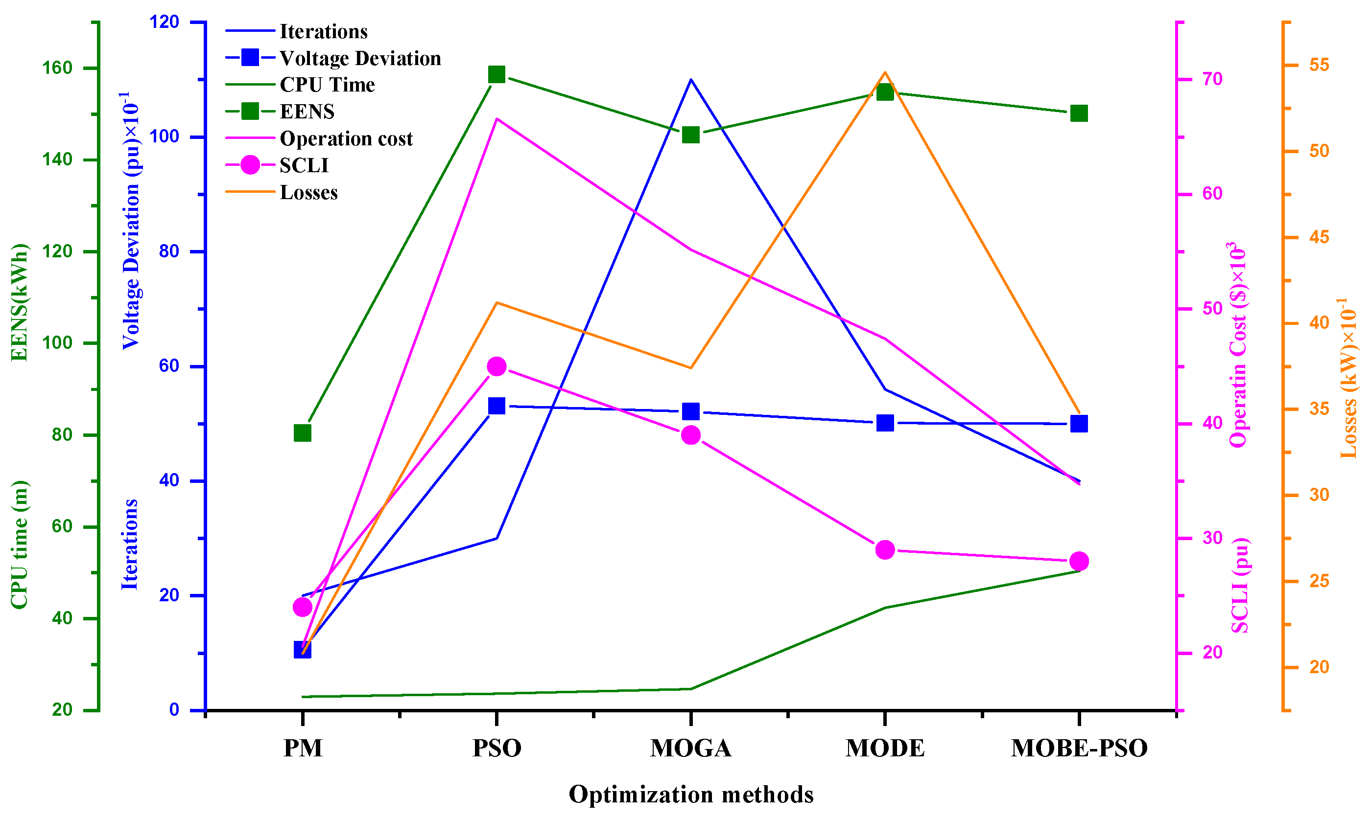
| CPU | Operation | Losses | Voltage | (EENS) | VSI | PLSF | SCLI | ||
| Optimization | Iterations | Times | Cost | (KW) | Deviation | ||||
| Method | (s) | ($) | (pu) | (KWh) | (pu) | (pu) | (pu) | ||
| (PM) | 20 | 1380 | 20,589.31 | 2.08 | 1.06 | 80.48 | 110.26 | 16.32 | 0.24 |
| P(PSO) | 30 | 1420 | 66581.51 | 4.12 | 5.31 | 158.62 | 97.19 | 14.26 | 0.45 |
| (MOGA) | 110 | 1480 | 55164.43 | 3.74 | 5.21 | 145.46 | 87.52 | 15.33 | 0.39 |
| (MODE) | 56 | 2541 | 47412.74 | 5.46 | 5.01 | 154.82 | 154.54 | 14.88 | 0.29 |
| (MOBE-PSO) | 40 | 3024 | 34718.87 | 3.48 | 5 | 150.18 | 117.73 | 15.61 | 0.28 |
| Indexes | Operating Cost ($) | Losses (kW) | Voltage Deviation (pu) | (EENS) (kWh) | VSI (pu) | Sum of Short Circuit-Level Changes (pu) | |
|---|---|---|---|---|---|---|---|
| Consideration Status | |||||||
| Proposed Method | 2804.55 | 0.84 | 2.21 | 118.32 | 9.91 | 0.52 | |
 | | | | | | ||
| [7,8] | 2856.39 | 1.24 | 3.21 | 215.21 | 1.22 | 7.98 | |
| | |  | | | ||
| [12,14] | 2934.41 | 9.87 | 4.35 | 110.21 | 3.73 | 5.21 | |
| | | | | | ||
| [24,25,27] | 3654.61 | 1.94 | 2.35 | 125.64 | 1.32 | 11.32 | |
| | | | | | ||
| Indexes | Operating Cost ($) | Losses (kW) | Voltage Deviation (pu) | (EENS) (kWh) | VSI (pu) | Sum of Short Circuit-Level Changes (pu) | |
|---|---|---|---|---|---|---|---|
| Consideration Status | |||||||
| Proposed Method | 20,589.31 | 2.08 | 1.06 | 80.48 | 110.26 | 0.24 | |
| | | | | | ||
| [7,8] | 20,474.76 | 2.28 | 5.45 | 334.91 | 78.21 | 5.23 | |
| | | | | | ||
| [12,14] | 19,643.21 | 11.34 | 6.28 | 78.25 | 65 | 4.12 | |
| | | | | | ||
| [24,25,27] | 2392.14 | 3.67 | 5.21 | 91.21 | 131.21 | 12.34 | |
| | | | | | ||
| Indexes | Operating Cost ($) | Losses (kW) | Voltage Deviation (pu) | (EENS) (kWh) | VSI (pu) | Sum of Short Circuit-Level Changes (pu) | |
|---|---|---|---|---|---|---|---|
| Consideration Status | |||||||
| Proposed Method | 4224.24 | 0.28 | 0.43 | 15.35 | 67.52 | 0.000 | |
| | | | | | ||
| [7,8] | 4321.69 | 1.021 | 1.31 | 65.28 | 21.62 | 2.84 | |
| | | | | | ||
| [12,14] | 4223.89 | 7.34 | 9.31 | 18.21 | 62.38 | 6.96 | |
| | | | | | ||
| [24,25,27] | 4721.33 | 0.97 | 2.10 | 19.94 | 63.46 | 8.32 | |
| | | | | | ||
Disclaimer/Publisher’s Note: The statements, opinions and data contained in all publications are solely those of the individual author(s) and contributor(s) and not of MDPI and/or the editor(s). MDPI and/or the editor(s) disclaim responsibility for any injury to people or property resulting from any ideas, methods, instructions or products referred to in the content. |
© 2023 by the authors. Licensee MDPI, Basel, Switzerland. This article is an open access article distributed under the terms and conditions of the Creative Commons Attribution (CC BY) license (https://creativecommons.org/licenses/by/4.0/).
Share and Cite
Al-Zaidi, W.K.M.; Inan, A. Optimal Placement of Battery Swapping Stations for Power Quality Improvement: A Novel Multi Techno-Economic Objective Function Approach. Energies 2024, 17, 110. https://doi.org/10.3390/en17010110
Al-Zaidi WKM, Inan A. Optimal Placement of Battery Swapping Stations for Power Quality Improvement: A Novel Multi Techno-Economic Objective Function Approach. Energies. 2024; 17(1):110. https://doi.org/10.3390/en17010110
Chicago/Turabian StyleAl-Zaidi, Waleed Khalid Mahmood, and Aslan Inan. 2024. "Optimal Placement of Battery Swapping Stations for Power Quality Improvement: A Novel Multi Techno-Economic Objective Function Approach" Energies 17, no. 1: 110. https://doi.org/10.3390/en17010110
APA StyleAl-Zaidi, W. K. M., & Inan, A. (2024). Optimal Placement of Battery Swapping Stations for Power Quality Improvement: A Novel Multi Techno-Economic Objective Function Approach. Energies, 17(1), 110. https://doi.org/10.3390/en17010110