An Open-Source Energy Arbitrage Model Involving Price Bands for Risk Hedging with Imperfect Price Signals

Abstract

The increased uptake of variable renewable energy sources has increased electricity price volatility in many energy pool markets, providing an opportunity for storage systems to profit through energy arbitrage. Comparison between the cost or value of storage systems engaging in energy arbitrage should be performed on a levelised basis due to differences in system lifetime. Existing energy arbitrage models with bid/offer curves and imperfect forecasting are typically computationally expensive and are impractical for calculating lifetime levelised cost metrics. In this work, an open-source modular energy arbitrage model with bid and offer curve inputs was developed for a lithium-ion battery energy storage system (BESS) and pumped hydro system (PHS) to analyse lifetime levelised cost and revenue. The mixed integer linear program scheduling module included a new piece-wise linearised description of PHS charging behaviour for rapid optimisation. A one-at-a-time sensitivity analysis indicated that levelised cost and revenue were highly sensitive to discharging efficiency. In a case study based on Australia’s National Electricity Market, imperfect forecasting with no risk hedging was found to increase levelised costs by up to 24% and decrease levelised revenue by up to 50% relative to perfect price forecasting, despite 95% of prices being forecast to be within $35/MWh of the actual trading price. BESS levelised costs were more significantly correlated with consistent low risk bids (Kendall Tau-b of 0.75), since the undiscounted capital costs contribute to a larger proportion of the overall costs than in the PHS systems.

1. Introduction

From 2016 to 2022, global wind and solar photovoltaic capacity had increased at an average of 12% and 22%, respectively, each year. By the end of 2022, these variable renewable energy (VRE) sources accounted for approximately 23% of the total installed electricity generation capacity [1].

A higher proportion of VRE sources in the energy mix has been correlated with an increase in price volatility within many wholesale electricity markets [2,3,4,5,6]. How the VRE capacity impacts electricity price volatility depends upon the market structure and demand during the hours of VRE generation. Recently, it has been found that wind generation during low demand hours tends to increase price volatility, while solar generation typically occurs during periods of high demand and may reduce price volatility [7,8,9].

Energy storage systems with the capacity to discharge for several hours, such as batteries and pumped hydro, are capable of providing an energy time-shifting service, ensuring that there is an adequate electricity supply when VREs are low [10,11]. When the increased VRE supply causes an increase in price volatility, there is the opportunity for storage systems to capitalise on the price spread through energy arbitrage by performing this time-shifting service.

Furthermore, ancillary services and contract markets can also constitute a large portion of storage system revenue. Despite only spot market arbitrage being considered in this paper, it is important to recognise that storage systems will participate in multiple markets simultaneously.

Existing arbitrage models in the literature broadly fit into two categories: simple models that ignore the risk of imperfect price forecasting but have low computational complexity, or complex model that manage the risk of imperfect price forecasting but can only reasonably be used to analyse short simulation periods. The simple models are capable of analysing the entire lifetime of an energy storage system, but often ignore important details such as the loss of revenue associated with imperfect price forecasting, battery degradation, or non-linear charging behaviours. The complex models may have increased accuracy, but the high computational complexity means that they cannot be reasonably used to calculate levelised cost of storage metrics over the lifetime of a system without extensive access to expensive supercomputing resources. Comparisons between storage systems with different lifetimes, degradation rates, and cycle behaviour must be performed on a levelised basis to enable a fair comparison of costs.

Many of the low-complexity arbitrage models in the literature assume perfect price forecasting to optimise storage system behaviour [12,13,14,15]. However, when imperfect price forecasting is used for energy arbitrage modelling instead, there will be a reduction in arbitrage revenue through two mechanisms: missed opportunities to schedule at optimal charging/discharging prices or dispatch during unfavourable pricing events.

Models for forecasting short-term electricity prices have typically reported errors of between 5% and 36% relative to the actual price [16]. When modelling arbitrage based on locational marginal pricing in Ontario, Antweiler [17] determined that revenue with perfect forecasting was double that predicted when using basic forecasting techniques. Improved forecasting techniques have suggested that between 81% and 85% of the potential arbitrage value can be obtained when uncertainty in the price signal exists [18,19,20].

Many analyses that consider imperfect price forecasting for energy arbitrage modelling assume that the storage system is guaranteed to win the bid or offer for each dispatch interval. Thatte et al. [21] explored the use of robust optimisation to manage price uncertainty and inform the day-ahead scheduling of capacity for a wind farm and energy storage system. Mixed integer linear programming (MILP) has also been used to model the scheduling of capacity for a cryogenic energy storage system [22] and a generic storage system [19] with imperfect price forecasting. A predictive price signal method that defines dynamic electricity price classes has been used to determine optimal intervals for scheduling battery capacity [23]. Battery control for arbitrage purposes has also been formulated as a Markov Decision Process to optimise the scheduling of capacity with imperfectly forecast prices [24] or co-optimising with the frequency control market based on historical prices [25]. Charging and discharging decisions for batteries with uncertain energy prices have also been optimised using a dynamic matrix-based program [26]. Electricity prediction errors of 12.5% were noted to halve arbitrage revenue under a sliding-window dynamic programming strategy that attempted to minimise battery degradation during scheduling [27]. The absence of a bid/offer price strategy reduces the scope of analysis that these models can perform for storage systems in real liberalised energy-pool markets.

The bid and offer price for a trading interval enables the storage system to hedge against the risk of dispatching during suboptimal intervals when uncertainty exists in the forecast spot prices. A comparison between a stochastic capacity-price bidding strategy and a deterministic capacity-only bidding strategy was performed by Kirshnamurthy et al. [28]. The authors found that the stochastic method typically obtained higher arbitrage revenue, but exposed the system to a higher level of risk. Tian et al. [29] developed a stochastic model that used downside risk constraints to define bid and offer curves for a PHS that hedge against risk when spot prices are uncertain. Li et al. [30] explored using a stochastic p-robust optimisation method instead of the downside risk constraints method to define the bid and offer price curves, noting that a 19% decline in profits could be associated with a 41% decrease in maximum relative regret.

An information gap decision theory (IGDT)-based risk-constrained strategy for developing bid and offer capacity-price curves of a price-taker compressed air energy storage system was found to be more profitable than a deterministic strategy [31]. The method was only used to analyse short-run costs and profits over a maximum period of 4 weeks. A similar analysis was performed using a robust optimisation for a price-maker-compressed air energy storage facility, with the robust-based strategy generally obtaining a higher revenue than a risk-neutral strategy [32].

Although the stochastic bid/offer price strategies for arbitrage models in the literature were found to be more profitable when compared with deterministic strategies, their computational time is expected to be much higher. This means that it is infeasible to fairly compare the cost of storage between different technologies, since this should be performed on a levelised basis.

Comparison between the cost or value of different electrical energy storage technologies should be performed on a levelised basis, taking account of the difference in system lifetime and the influence of power capacity and energy capacity or storage duration on capital costs. The analysis in this study will determine the impact of a simple price band risk hedging strategy on the required average discharge price (RADP) and available average discharge price (AADP) of the levelised cost of storage metrics, as defined by Belderbos et al. [33]. These two metrics define the levelised long-run marginal cost and revenue of the system, respectively, and are an important step in estimating the return on investment of a hypothetical system.

An open-source modular energy arbitrage model has been developed which uses price band curves for risk hedging in the presence of imperfect price signals. This new model balances the accuracy of non-linear models that manage the risk of imperfect price forecasts with the computational speed of a simple deterministic scheduling algorithm. The new model includes the following novel features compared to existing open-source arbitrage models:

• The MILP scheduling model applies a piece-wise linearisation process to a pumped hydro storage (PHS) system. This allows the non-linear charging behaviour of the PHS to be approximated during scheduling, taking advantage of the speed of MILP optimisation. The piece-wise linearisation process will be a more accurate approximation than assuming the constant linear behaviour of the PHS in all operating conditions.
• Battery degradation has been considered within the piece-wise linearised description of a battery developed by Sakti et al. [14]. This allows for changes to battery voltage efficiency over its lifetime to be included within the MILP scheduling algorithm while maintaining an accurate approximation of the non-linear charging behaviour.
• The rapid optimisation provided by the MILP scheduling algorithm, along with the additional accuracy provided by the non-linear charging model and piece-wise linear approximation of charging behaviour during scheduling, allows the simulation period to cover the entire lifetime of each storage system. This allows for computation of the lifetime-levelised cost of storage metrics (RADP and AADP), enabling a comparison between the arbitrage revenue of storage systems with different lifetimes, cycling behaviour, and degradation rates.
• Charging and discharging efficiencies are considered separately and modelled according to non-linear functions, where appropriate. Some previous studies have assumed the use of a round-trip efficiency during dispatch [19,34], though this may be inappropriate for modelling arbitrage revenue in wholesale energy markets that have a high price ceiling.
• The code for the model is available open-source on Github. The current version contains a scheduling and charging model for a Li-ion BESS and PHS. The modification of the arbitrage model to analyse alternative storage systems, such as the compressed air energy storage or other battery technologies, would only require the development of bespoke scheduling and charging modules that can be directly integrated with the rest of the system.

It should also be noted that the modelling results discussed in this paper may not be appropriate when considering unusual events such as the COVID-19 pandemic, the global energy price response to the Russian invasion of Ukraine, a hypothetical oil embargo or a nuclear catastrophe such as Fukushima. Arbitrage models are most appropriately employed for understanding the behaviour of a system under different conditions, rather than providing accurate estimates of lifetime revenue.

The mathematical arbitrage model developed for this study is outlined in Section 2. In Section 3, a sensitivity analysis is presented, and the model is used to determine the impact of a static risk level on the levelised cost of storage metrics for a hypothetical battery energy storage system (BESS) and PHS operating in the Australian National Electricity Market (NEM).

2. Model Details

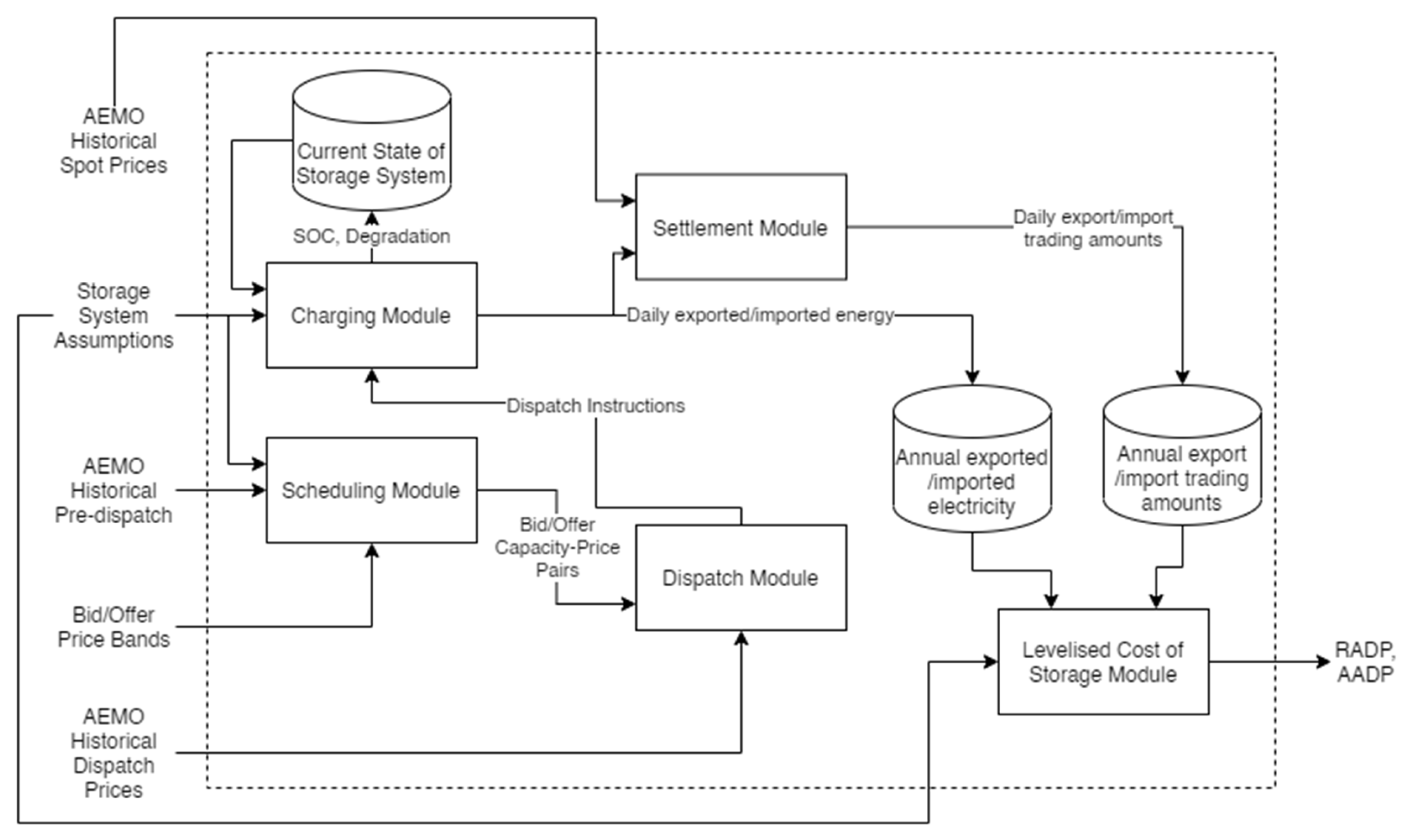
2.1. Arbitrage Model

At a high level, this arbitrage model can be described as a set of interconnected modules (see Figure 1). The system is designed to perform day-ahead scheduling. Optimisation for scheduling is performed by a MILP programmed using the Pyomo [35,36] modelling package for Python and solved using the COIN-OR Branch-and-Cut (CBC) solver [37]. It is assumed that the storage system is a price-taker during dispatch.

The dispatch module generates a set of dispatch instructions for the trading day which are sent to the storage system’s charging module. The charging module runs through each dispatch interval in series, attempting to follow all dispatch instructions whilst operating within the constraints of the system. If the storage system is a BESS, then the capacity fading and efficiency fading at each interval are also calculated to update the current state of the storage system. Once the charging module reaches the end of the trading day, it sends a list of the charged and discharged energies for each dispatch interval to the settlement module. Based upon the spot prices for the trading day, the settlement module determines the trading amounts in each dispatch interval. Scheduling is then repeated for the upcoming trading day.

The daily energy throughputs and trading amounts are stored as aggregate values until the end of the system life. Using the lifetime discharged energy, costs and gross revenue, the levelised cost of the storage module determines the long-run marginal costs and revenue made by the simulated system.

Although scheduling occurs before charging within the simulation, it is necessary to understand the charging behaviour of the system before we can define the scheduling constraints.

2.1.1. Charging Module

In general, the BESS and PHS charging modules determine what SOC the system would reach if it followed the dispatch instruction for a given 5-min dispatch interval t (i.e., $SO{C}_t^{\mathrm{t}\mathrm{e}\mathrm{s}\mathrm{t}}$). In Equation (1), the SOC at the start of the interval, $SO{C}_t^{\mathrm{p}\mathrm{r}\mathrm{e}}$, is initialised to be 50% (i.e., $SO{C}_{\mathrm{i}\mathrm{n}\mathrm{i}\mathrm{t}\mathrm{i}\mathrm{a}\mathrm{l}}$) in the first interval or the SOC at the end t − 1 for all other intervals. If the system can move from $SO{C}_t^{\mathrm{p}\mathrm{r}\mathrm{e}}$ to $SO{C}_t^{\mathrm{t}\mathrm{e}\mathrm{s}\mathrm{t}}$ without violating the constraints of the system, then it follows the dispatch instruction. Otherwise, it ignores the dispatch instruction, as per Equation (2).

$$SO{C}_t^{\mathrm{p}\mathrm{r}\mathrm{e}}=\left\{\begin{array}{l}SO{C}_{\mathrm{i}\mathrm{n}\mathrm{i}\mathrm{t}\mathrm{i}\mathrm{a}\mathrm{l}}, t=1\\ SO{C}_{t-1}, t>1\end{array}\right.$$

(1)

$$SO{C}_t=\left\{\begin{array}{l}SO{C}_t^{\mathrm{t}\mathrm{e}\mathrm{s}\mathrm{t}}, SO{C}_{\mathrm{m}\mathrm{i}\mathrm{n}}\le SO{C}_t^{\mathrm{t}\mathrm{e}\mathrm{s}\mathrm{t}}\le SO{C}_{\mathrm{m}\mathrm{a}\mathrm{x}}\\ SO{C}_{t-1}, SO{C}_t^{\mathrm{t}\mathrm{e}\mathrm{s}\mathrm{t}}\le SO{C}_{\mathrm{m}\mathrm{i}\mathrm{n}} or SO{C}_t^{\mathrm{t}\mathrm{e}\mathrm{s}\mathrm{t}}\ge SO{C}_{\mathrm{m}\mathrm{a}\mathrm{x}}\end{array}\right.$$

(2)

Pumped Hydro Storage Charging Module

Individual pumps and turbines are indexed by g and h, respectively. The PHS is assumed to consist of pumps independent of the turbines, and the turbines are assumed to be synchronous rather than of a variable speed. Ternary PHSs have a shorter transient time when changing between pumping and generating modes, which is expected to be ideal in volatile electricity markets. Furthermore, ternary systems typically have a higher peak efficiency than variable speed systems, which should maximise discharging profits during high-price events [38]. The dispatched power of each pump and turbine, defined by Equations (3) and (4), is dependent on whether the PHS can perform the dispatch instructions it receives from the dispatch model. The charging power of pump g for time interval t, given by $P_{t,g}^{\mathrm{c}}$ [MW], is equal to the dispatch instruction issued to the load, $P_{\mathrm{l}\mathrm{o}\mathrm{a}\mathrm{d},t,g}^{\mathrm{d}\mathrm{i}\mathrm{s}\mathrm{p}}$ [MW], if it would result in a SOC within the bounds of the system. The discharging behaviour of turbine h is similarly defined by the dispatch instruction issued to the generator, $P_{\mathrm{g}\mathrm{e}\mathrm{n},t,h}^{\mathrm{d}\mathrm{i}\mathrm{s}\mathrm{p}}$ [MW], if it is capable of reaching the new SOC.

$$P_{t,g}^{\mathrm{c}}=\left\{\begin{array}{c}{P}_{\mathrm{l}\mathrm{o}\mathrm{a}\mathrm{d},t,g}^{\mathrm{d}\mathrm{i}\mathrm{s}\mathrm{p}}, SO{C}_{\mathrm{m}\mathrm{i}\mathrm{n}}\le SO{C}_t^{\mathrm{t}\mathrm{e}\mathrm{s}\mathrm{t}}\le SO{C}_{\mathrm{m}\mathrm{a}\mathrm{x}}\\ 0, SO{C}_t^{\mathrm{t}\mathrm{e}\mathrm{s}\mathrm{t}}\le SO{C}_{\mathrm{m}\mathrm{i}\mathrm{n}} \mathrm{or} SO{C}_t^{\mathrm{t}\mathrm{e}\mathrm{s}\mathrm{t}}\ge SO{C}_{\mathrm{m}\mathrm{a}\mathrm{x}}\end{array}\right.$$

(3)

$$P_{t,h}^{\mathrm{d}}=\left\{\begin{array}{c}{P}_{\mathrm{g}\mathrm{e}\mathrm{n},t,h}^{\mathrm{d}\mathrm{i}\mathrm{s}\mathrm{p}}, SO{C}_{\mathrm{m}\mathrm{i}\mathrm{n}}\le SO{C}_t^{\mathrm{t}\mathrm{e}\mathrm{s}\mathrm{t}}\le SO{C}_{\mathrm{m}\mathrm{a}\mathrm{x}}\\ 0, SO{C}_t^{\mathrm{t}\mathrm{e}\mathrm{s}\mathrm{t}}\le SO{C}_{\mathrm{m}\mathrm{i}\mathrm{n}} \mathrm{or} SO{C}_t^{\mathrm{t}\mathrm{e}\mathrm{s}\mathrm{t}}\ge SO{C}_{\mathrm{m}\mathrm{a}\mathrm{x}}\end{array}\right.$$

(4)

The PHS charging behaviour is non-linear and consists of a steady-state calculation of SOC with a transient adjustment. Updates to the upper reservoir are based upon Equation (5). The SOC at the end of the time interval is based on the length of the dispatch interval, $\tau$ [hours], multiplied by the steady-state flow rate through the pumps and turbines, as defined by $Q_{t,g}^{\mathrm{p}}$ and $Q_{t,h}^{\mathrm{t}}$ [m³/s], respectively. The transient adjustments to the reservoir volume, $∆V_t^{\mathrm{p}}$ and $∆V_t^{\mathrm{t}}$ [m³], account for the transition times required to switch between pumping and generating. The maximum volume of the upper reservoir is given by $V^{\mathrm{u}\mathrm{r}}$ [m³].

$$SO{C}_t^{\mathrm{t}\mathrm{e}\mathrm{s}\mathrm{t}}=\frac{1}{V^{\mathrm{u}\mathrm{r}}}\left(3600·\tau ·\left({\sum }_g\left(Q_{t,g}^{\mathrm{p}}\right)-{\sum }_h\left(Q_{t,h}^{\mathrm{t}}\right)\right)+d{V}_t^{\mathrm{p}}+d{V}_t^{\mathrm{t}}\right)+SO{C}_t^{\mathrm{p}\mathrm{r}\mathrm{e}}$$

(5)

The steady-state calculation is based upon the pumped hydro model developed by Mousavi et al. [39]. Equations (6) and (7) calculate the flow rate of a pump or turbine unit based upon the net head ($H_t^{\mathrm{p}}$ or $H_t^{\mathrm{t}}$), efficiency of the unit ($\eta$) and dispatch instruction. Water density ($\rho$) and acceleration due to gravity ($g$) are assumed to be 997 [kg/m³] and 9.81 [m/s], respectively. The net heads of the pumps and turbines are determined using Equations (8) and (9), where the gross head is adjusted by the head loss ($H_t^{\mathrm{p}\mathrm{l}}$ or $H_t^{\mathrm{t}\mathrm{l}}$ [m]) for the associated penstock within that interval. The gross head is defined by the height difference between the bottom of the upper reservoir and top of the lower reservoir ($h^{\mathrm{r}}$ [m]), the water level of the upper reservoir ($h_t^{\mathrm{u}\mathrm{w}\mathrm{l}}$ [m]), the maximum possible water height in the lower reservoir ($h^{\mathrm{l}\mathrm{r}}$ [m]) and the water level of the lower reservoir ($h_t^{\mathrm{l}\mathrm{w}\mathrm{l}}$ [m]).

$$Q_{t,g}^{\mathrm{p}}=\frac{P_{\mathrm{l}\mathrm{o}\mathrm{a}\mathrm{d},t,g}^{\mathrm{d}\mathrm{i}\mathrm{s}\mathrm{p}}·{10}^6·{\eta }_{t,g}^{\mathrm{p}}}{H_t^{\mathrm{p}}·\rho ·g}$$

(6)

$$Q_{t,h}^{\mathrm{t}}=\frac{P_{\mathrm{g}\mathrm{e}\mathrm{n},t,h}^{\mathrm{d}\mathrm{i}\mathrm{s}\mathrm{p}}·{10}^6}{H_t^{\mathrm{t}}·\rho ·g·{\eta }_{t,h}^{\mathrm{t}}}$$

(7)

$$H_t^{\mathrm{p}}=h^{\mathrm{r}}+h^{\mathrm{u}\mathrm{w}\mathrm{l}}+h^{\mathrm{l}\mathrm{r}}-h^{\mathrm{l}\mathrm{w}\mathrm{l}}+H_t^{\mathrm{p}\mathrm{l}}$$

(8)

$$H_t^t=h^{\mathrm{r}}+h^{\mathrm{u}\mathrm{w}\mathrm{l}}+h^{\mathrm{l}\mathrm{r}}-h^{\mathrm{l}\mathrm{w}\mathrm{l}}-H_t^{\mathrm{t}\mathrm{l}}$$

(9)

The head loss is dependent upon the size, materials, and shape of the penstock (defined by resistance coeffient $K$ of the pipes and fittings, penstock pipe diameter $PD$ [m], friction factor $F$ and penstock pipe length $L$ [m]), as well as the velocity of the water ($WV$ [m/s]) required to achieve the desired flow rate ($Q$ [m³/s]). The friction factor is based on the Reynolds number ($Re$) and absolute roughness ($\epsilon$ [m]) of the penstock. The dynamic viscosity of water ($\mu$) is assumed to be $8.9\times {10}^{-4}$ [Pa·s]. Further details of these parameters can be found in [39]. The pump head loss is calculated according to Equations (10)–(15), while the turbine head loss is calculated from Equations (16)–(21). The model used for this analysis assumes a single penstock for the pumps and another for the turbines, although it would be possible to define multiple penstocks by indexing the parameters in the relevant equations. Different pumps and turbines could then have different net heads due to any assymetry between their associated penstocks.

$$H_t^{\mathrm{p}\mathrm{l}}=\frac{K_t^{\mathrm{p}}·{\left({WV}_t^{\mathrm{p}}\right)}^2}{2g}$$

(10)

$${WV}_t^{\mathrm{p}}=\frac{{\sum }_g{Q}_{t,g}^{\mathrm{p}}}{0.25·\pi ·{\left({PD}^{\mathrm{p}}\right)}^2}$$

(11)

$$K_t^{\mathrm{p}}=K_t^{\mathrm{p},\mathrm{p}\mathrm{i}\mathrm{p}\mathrm{e}}+K^{\mathrm{p},\mathrm{f}\mathrm{i}\mathrm{t}\mathrm{t}\mathrm{i}\mathrm{n}\mathrm{g}\mathrm{s}}$$

(12)

$$K_t^{\mathrm{p},\mathrm{p}\mathrm{i}\mathrm{p}\mathrm{e}}=\frac{F_t^{\mathrm{p}}·L^{\mathrm{p}}}{{PD}^{\mathrm{p}}}$$

(13)

$$F_t^{\mathrm{p}}={\left[1.8·\log \left(\frac{6.9}{R{e}_t^{\mathrm{p}}}+{\left(\frac{{\epsilon }^{\mathrm{p}}/{PD}^{\mathrm{p}}}{3.7}\right)}^{1.11}\right)\right]}^{-2}$$

(14)

$$R{e}_t^{\mathrm{p}}=\frac{\rho ·{WV}_t^{\mathrm{p}}·{PD}^{\mathrm{p}}}{\mu }$$

(15)

$$H_t^{\mathrm{t}\mathrm{l}}=\frac{K_t^{\mathrm{t}}·{\left({WV}_t^{\mathrm{t}}\right)}^2}{2g}$$

(16)

$${WV}_t^{\mathrm{t}}=\frac{{\sum }_h{Q}_{t,h}^{\mathrm{t}}}{0.25·\pi ·{\left({PD}^{\mathrm{t}}\right)}^2}$$

(17)

$$K_t^{\mathrm{t}}=K_t^{\mathrm{t},\mathrm{p}\mathrm{i}\mathrm{p}\mathrm{e}}+K^{\mathrm{t},\mathrm{f}\mathrm{i}\mathrm{t}\mathrm{t}\mathrm{i}\mathrm{n}\mathrm{g}\mathrm{s}}$$

(18)

$$K_t^{\mathrm{t},\mathrm{p}\mathrm{i}\mathrm{p}\mathrm{e}}=\frac{F_t^{\mathrm{t}}·L^{\mathrm{t}}}{{PD}^{\mathrm{t}}}$$

(19)

$$F_t^{\mathrm{t}}={\left[1.8·\log \left(\frac{6.9}{R{e}_t^{\mathrm{t}}}+{\left(\frac{{\epsilon }^{\mathrm{t}}/{PD}^{\mathrm{t}}}{3.7}\right)}^{1.11}\right)\right]}^{-2}$$

(20)

$$R{e}_t^{\mathrm{t}}=\frac{\rho ·{WV}_t^{\mathrm{t}}·{PD}^{\mathrm{t}}}{\mu }$$

(21)

The efficiency of the pumping system is assumed to be 91%, as per Equation (22). The constant efficiency is considered appropriate since pumps typically operate at their rated conditions [40]. The value of 91% is based upon the efficiency losses due to the pump, motor, and transformer losses, as outlined by Chen [41]. The water conductor losses described by Chen are captured by the head loss calculation. The turbine efficiency is empirically derived by fitting parameters (${\xi }_n^{\mathrm{t}}$) to the Francis turbine hill plot in Bostan et al. [42]. The relative flow rate ($Q_{t,h}^{\mathrm{t},\mathrm{r}\mathrm{e}\mathrm{l}}$ [m³/s]) is based on the actual flow rate ($Q_{t,h}^{\mathrm{t}}$ [m³/s]) relative to the flow rate at peak efficiency ($Q_{\mathrm{p}\mathrm{e}\mathrm{a}\mathrm{k},h}^{\mathrm{t}}$ [m³/s]), calculated in Equation (23). The empirical function fitted according to Equation (24) assumes that the turbine is operating at a nominal head. Although turbine efficiency is technically also a function of net head, it is significantly more dependent upon flow rate; thus, the assumption is considered reasonable for this analysis [43]. Flow rate and the associated head loss are calculated by finding the steady state solution to Equations (10)–(24) [39].

$${\eta }_{t,g}^{\mathrm{p}}=0.91$$

(22)

$$Q_{t,h}^{\mathrm{t},\mathrm{r}\mathrm{e}\mathrm{l}}=\frac{Q_{t,h}^{\mathrm{t}}}{Q_{\mathrm{p}\mathrm{e}\mathrm{a}\mathrm{k},h}^{\mathrm{t}}}$$

(23)

$${\eta }_{t,h}^{\mathrm{t}}={\displaystyle {\sum }_{n=0}^4}\left({\xi }_n^{\mathrm{t}}·{\left(Q_{t,h}^{\mathrm{t},\mathrm{r}\mathrm{e}\mathrm{l}}\right)}^n\right)$$

(24)

The transient adjustment to the SOC considers the time required to change the flow rate. The ramp times ($R{T}^{\mathrm{T}\mathrm{N}\mathrm{L}\to \mathrm{T}}$, $R{T}^{\mathrm{T}\to \mathrm{T}\mathrm{N}\mathrm{L}}$, $R{T}^{\mathrm{T}\mathrm{N}\mathrm{L}\to \mathrm{P}}$, and $R{T}^{\mathrm{P}\to \mathrm{T}\mathrm{N}\mathrm{L}}$ [s]) between turbine operation, turbine-no-load and pump operation are defined as parameters. The ramp time for an individual unit during a given interval is calculated from Equation (25) or Equation (26). The upper reservoir water volume is then adjusted according to Equations (27) and (28) to account for the transient behaviour.

$$R{T}_{t,h}^{\mathrm{t}}=\left\{\begin{array}{c}\left(Q_{t,h}^{\mathrm{t}}-Q_{t-1,h}^{\mathrm{t}}\right)·\frac{R{T}^{\mathrm{T}\mathrm{N}\mathrm{L}\to \mathrm{T}}}{Q_{\mathrm{p}\mathrm{e}\mathrm{a}\mathrm{k},h}^{\mathrm{t}}}, Q_{t,h}^{\mathrm{t}}\ge Q_{t-1,h}^{\mathrm{t}}\\ \left(Q_{t-1,h}^{\mathrm{t}}-Q_{t,h}^{\mathrm{t}}\right)·\frac{R{T}^{\mathrm{T}\to \mathrm{T}\mathrm{N}\mathrm{L}}}{Q_{\mathrm{p}\mathrm{e}\mathrm{a}\mathrm{k},h}^{\mathrm{t}}}, Q_{t-1,h}^{\mathrm{t}}>Q_{t,h}^{\mathrm{t}}\end{array}\right.$$

(25)

$${RT}_{t,g}^{\mathrm{p}}=\left\{\begin{array}{c}\left(Q_{t,g}^{\mathrm{p}}-Q_{t-1,g}^{\mathrm{p}}\right)·\frac{R{T}^{\mathrm{T}\mathrm{N}\mathrm{L}\to \mathrm{P}}}{Q_{\mathrm{p}\mathrm{e}\mathrm{a}\mathrm{k},g}^{\mathrm{p}}}, Q_{t,g}^{\mathrm{p}}\ge Q_{t-1,g}^{\mathrm{p}}\\ \left(Q_{t-1,g}^{\mathrm{p}}-Q_{t,g}^{\mathrm{p}}\right)·\frac{R{T}^{\mathrm{P}\to \mathrm{T}\mathrm{N}\mathrm{L}}}{Q_{\mathrm{p}\mathrm{e}\mathrm{a}\mathrm{k},g}^{\mathrm{t}}}, Q_{t-1,g}^{\mathrm{p}}>Q_{t,g}^{\mathrm{p}}\end{array}\right.$$

(26)

$$d{V}_t^{\mathrm{p}}=\left\{\begin{array}{l}{\sum }_g\frac{{RT}_{t,g}^{\mathrm{p}}}{2}·\left(Q_{t-1,g}^{\mathrm{p}}-Q_{t,g}^{\mathrm{p}}\right), {\sum }_h{Q}_{t,h}^{\mathrm{t}}={\sum }_h{Q}_{t-1,h}^{\mathrm{t}}\\ {\sum }_g\frac{{RT}_{t,g}^{\mathrm{p}}}{2}·\left(Q_{t-1,g}^{\mathrm{p}}-Q_{t,g}^{\mathrm{p}}\right), {\sum }_g{Q}_{t,g}^{\mathrm{p}}<{\sum }_g{Q}_{t-1,g}^{\mathrm{p}} \mathrm{a}\mathrm{n}\mathrm{d} {\sum }_h{Q}_{t,h}^{\mathrm{t}}>{\sum }_h{Q}_{t-1,h}^{\mathrm{t}}\\ {\sum }_g\left(\frac{{RT}_{t,g}^{\mathrm{p}}}{2}+\max \left(R{T}_{t,h}^{\mathrm{t}}\right)\right)·\left(Q_{t-1,g}^{\mathrm{p}}-Q_{t,g}^{\mathrm{p}}\right),{\sum }_g{Q}_{t,g}^{\mathrm{p}}>{\sum }_g{Q}_{t-1,g}^{\mathrm{p}} \mathrm{a}\mathrm{n}\mathrm{d} {\sum }_h{Q}_{t,h}^{\mathrm{t}}<{\sum }_h{Q}_{t-1,h}^{\mathrm{t}}\\ 0, {\sum }_g{Q}_{t,g}^{\mathrm{p}}={\sum }_g{Q}_{t-1,g}^{\mathrm{p}}\end{array}\right.$$

(27)

$$d{V}_t^{\mathrm{t}}=\left\{\begin{array}{l}{\sum }_h\frac{{RT}_{t,h}^{\mathrm{t}}}{2}·\left(Q_{t,h}^{\mathrm{t}}-Q_{t-1,h}^{\mathrm{t}}\right), {\sum }_g{Q}_{t,g}^{\mathrm{p}}={\sum }_g{Q}_{t-1,g}^{\mathrm{p}}\\ {\sum }_h\frac{{RT}_{t,h}^{\mathrm{t}}}{2}·\left(Q_{t,h}^{\mathrm{t}}-Q_{t-1,h}^{\mathrm{t}}\right), {\sum }_g{Q}_{t,g}^{\mathrm{p}}>{\sum }_g{Q}_{t-1,g}^{\mathrm{p}} \mathrm{and} {\sum }_h{Q}_{t,h}^{\mathrm{t}}<{\sum }_h{Q}_{t-1,h}^{\mathrm{t}}\\ {\sum }_h\left(\frac{{RT}_{t,h}^{\mathrm{t}}}{2}+\max \left(R{T}_{t,g}^{\mathrm{p}}\right)\right)·\left(Q_{t,h}^{\mathrm{t}}-Q_{t-1,h}^{\mathrm{t}}\right),{\sum }_g{Q}_{t,g}^{\mathrm{p}}<{\sum }_g{Q}_{t-1,g}^{\mathrm{p}} \mathrm{a}\mathrm{n}\mathrm{d} {\sum }_h{Q}_{t,h}^{\mathrm{t}}>{\sum }_h{Q}_{t-1,h}^{\mathrm{t}}\\ 0, {\sum }_h{Q}_{t,h}^{\mathrm{t}}={\sum }_h{Q}_{t-1,h}^{\mathrm{t}}\end{array}\right.$$

(28)

Battery Energy Storage System Charging Module

The BESS modelled for this analysis is assumed to consist of lithium-ion cells. The voltage of the BESS is measured across the inverters before it is stepped up by the transformers for distribution or transmission.

The dispatched capacity for any interval t is dependent upon whether the BESS can operate at that power without exceeding the SOC bounds. The relationship between dispatched capacity and the dispatch instructions is provided in Equations (29) and (30).

$$P_t^{\mathrm{c}}=\left\{\begin{array}{c}{P}_{\mathrm{l}\mathrm{o}\mathrm{a}\mathrm{d},t}^{\mathrm{d}\mathrm{i}\mathrm{s}\mathrm{p}}, SO{C}_{\mathrm{m}\mathrm{i}\mathrm{n}}\le SO{C}_t^{\mathrm{t}\mathrm{e}\mathrm{s}\mathrm{t}}\le SO{C}_{\mathrm{m}\mathrm{a}\mathrm{x}}\\ 0, SO{C}_t^{\mathrm{t}\mathrm{e}\mathrm{s}\mathrm{t}}\le SO{C}_{\mathrm{m}\mathrm{i}\mathrm{n}} \mathrm{or} SO{C}_t^{\mathrm{t}\mathrm{e}\mathrm{s}\mathrm{t}}\ge SO{C}_{\mathrm{m}\mathrm{a}\mathrm{x}}\end{array}\right.$$

(29)

$$P_t^{\mathrm{d}}=\left\{\begin{array}{c}{P}_{\mathrm{g}\mathrm{e}\mathrm{n},t}^{\mathrm{d}\mathrm{i}\mathrm{s}\mathrm{p}}, SO{C}_{\mathrm{m}\mathrm{i}\mathrm{n}}\le SO{C}_t^{\mathrm{t}\mathrm{e}\mathrm{s}\mathrm{t}}\le SO{C}_{\mathrm{m}\mathrm{a}\mathrm{x}}\\ 0, SO{C}_t^{\mathrm{t}\mathrm{e}\mathrm{s}\mathrm{t}}\le SO{C}_{\mathrm{m}\mathrm{i}\mathrm{n}} \mathrm{or} SO{C}_t^{\mathrm{t}\mathrm{e}\mathrm{s}\mathrm{t}}\ge SO{C}_{\mathrm{m}\mathrm{a}\mathrm{x}}\end{array}\right.$$

(30)

The efficiency of the BESS is defined to consist of a voltage efficiency (${\eta }_t^{\mathrm{v}\mathrm{o}\mathrm{l}\mathrm{t}}$), representing the electrochemical losses of the battery, and the system efficiency (${\eta }^{\mathrm{s}\mathrm{y}\mathrm{s}}$), defining the auxiliary losses of the storage system. The voltage efficiency in Equation (31) and non-linear charging behaviour in Equation (32) are based upon the simplified electrical energy storage system representation developed by Sakti et al. [14] and Darling et al. [44]. The system efficiency is assumed to be constant within the simplified model, though it is important to note that auxiliary losses are dependent upon the dynamic thermal management of the system [45]. The energy capacity of the battery is defined by $C{E}^{\mathrm{b}\mathrm{a}\mathrm{t}\mathrm{t}}$ [MWh], the nominal voltage by $U_{\mathrm{n}\mathrm{o}\mathrm{m}}^{\mathrm{b}\mathrm{a}\mathrm{t}\mathrm{t}}$ [V], the voltage for a given time interval by $U_t^{\mathrm{b}\mathrm{a}\mathrm{t}\mathrm{t}}$ [V], the energy capacity of each cell by $C{E}^{\mathrm{c}\mathrm{e}\mathrm{l}\mathrm{l}}$ [MWh], and the internal resistance of the cells by ${ir}_t^{\mathrm{c}\mathrm{e}\mathrm{l}\mathrm{l}}$ [Ω].

$${\eta }_t^{\mathrm{v}\mathrm{o}\mathrm{l}\mathrm{t}}=\frac{1}{2}+\sqrt{\frac{1}{4}-\frac{\left(P_{\mathrm{g}\mathrm{e}\mathrm{n},t}^{\mathrm{d}\mathrm{i}\mathrm{s}\mathrm{p}}+P_{\mathrm{l}\mathrm{o}\mathrm{a}\mathrm{d},t}^{\mathrm{d}\mathrm{i}\mathrm{s}\mathrm{p}}\right)}{{\eta }^{\mathrm{s}\mathrm{y}\mathrm{s}}·SO{C}_t^{\mathrm{t}\mathrm{e}\mathrm{s}\mathrm{t}}·C{E}^{\mathrm{b}\mathrm{a}\mathrm{t}\mathrm{t}}}·{\left(\frac{U_{\mathrm{n}\mathrm{o}\mathrm{m}}^{\mathrm{b}\mathrm{a}\mathrm{t}\mathrm{t}}}{U_t^{\mathrm{b}\mathrm{a}\mathrm{t}\mathrm{t}}}\right)}^2·\frac{{ir}_t^{\mathrm{c}\mathrm{e}\mathrm{l}\mathrm{l}}·C{E}^{\mathrm{c}\mathrm{e}\mathrm{l}\mathrm{l}}}{U_{\mathrm{n}\mathrm{o}\mathrm{m}}^{\mathrm{c}\mathrm{e}\mathrm{l}\mathrm{l}}}}$$

(31)

$$SO{C}_t^{\mathrm{t}\mathrm{e}\mathrm{s}\mathrm{t}}=SO{C}_t^{\mathrm{p}\mathrm{r}\mathrm{e}}-\frac{1}{C{E}^{\mathrm{b}\mathrm{a}\mathrm{t}\mathrm{t}}}·\left(\frac{P_{\mathrm{g}\mathrm{e}\mathrm{n},t}^{\mathrm{d}\mathrm{i}\mathrm{s}\mathrm{p}}}{{\eta }_t^{\mathrm{v}\mathrm{o}\mathrm{l}\mathrm{t}}·{\eta }^{\mathrm{s}\mathrm{y}\mathrm{s}}}-{\eta }_t^{\mathrm{v}\mathrm{o}\mathrm{l}\mathrm{t}}·{\eta }^{\mathrm{s}\mathrm{y}\mathrm{s}}·P_{\mathrm{l}\mathrm{o}\mathrm{a}\mathrm{d},t}^{\mathrm{d}\mathrm{i}\mathrm{s}\mathrm{p}}\right)·\tau$$

(32)

The open-circuit voltage of each cell is defined by Equation (33). An analysis of methods for empirically fitting open-circuit voltage characteristic curves for lithium-ion batteries by Zhang et al. [46] suggested that a fourth-order Gaussian model produced the lowest root-mean-square error compared to the other fitting methods. The general Gaussian model for fitting the characteristic curve is provided in Equation (33), with n = 4 for the purposes of this analysis. Fitting parameters $\xi$, $\varphi$ and $\chi$ are used to define the characteristic curve. The nominal voltage is defined as the open-circuit voltage at 50% SOC, as per Equation (34). The open-circuit voltage of the entire BESS before it is stepped up is assumed to be equal to the sum of open-circuit voltages of the cells in series (see Equation (35)). The number of cells in series is given by $N^{\mathrm{s}\mathrm{e}\mathrm{r}\mathrm{i}\mathrm{e}\mathrm{s}}$. The resistance in the battery created by making cell connections is ignored for the purposes of this analysis [14].

$$U_t^{\mathrm{c}\mathrm{e}\mathrm{l}\mathrm{l}}={\displaystyle {\sum }_{nn=1}^n}{\xi }_n^{\mathrm{c}\mathrm{e}\mathrm{l}\mathrm{l}}·\exp \left(-{\left(\frac{SO{C}_t^{\mathrm{t}\mathrm{e}\mathrm{s}\mathrm{t}}-{\varphi }_n^{\mathrm{c}\mathrm{e}\mathrm{l}\mathrm{l}}}{{\chi }_n^{\mathrm{c}\mathrm{e}\mathrm{l}\mathrm{l}}}\right)}^2\right)$$

(33)

$$U_{\mathrm{n}\mathrm{o}\mathrm{m}}^{\mathrm{c}\mathrm{e}\mathrm{l}\mathrm{l}}={\displaystyle {\sum }_{nn=1}^n}{\xi }_n^{\mathrm{c}\mathrm{e}\mathrm{l}\mathrm{l}}·\exp \left(-{\left(\frac{0.5-{\varphi }_n^{\mathrm{c}\mathrm{e}\mathrm{l}\mathrm{l}}}{{\chi }_n^{\mathrm{c}\mathrm{e}\mathrm{l}\mathrm{l}}}\right)}^2\right)$$

(34)

$$U_t^{\mathrm{b}\mathrm{a}\mathrm{t}\mathrm{t}}=U_t^{\mathrm{c}\mathrm{e}\mathrm{l}\mathrm{l}}{N}^{\mathrm{s}\mathrm{e}\mathrm{r}\mathrm{i}\mathrm{e}\mathrm{s}}$$

(35)

Lithium-ion batteries are expected to experience both capacity fading and efficiency fading. The end-of-life criterion for a lithium-ion battery is typically defined to be degradation to 80% of its original energy capacity [47,48,49]. Furthermore, the internal resistance of an LFP/C battery cell held at 50% SOC at 25 °C is expected to increase by 71% over a 20-year period [50]. As shown in Equation (31), an increase in internal resistance would directly result in an increase in electrochemical losses.

Capacity fading in lithium-ion batteries is typically separated into two components: calendar aging and cycle aging. The empirical model developed by Petit et al. [51], originally based upon the work of Wang et al. [52], is used as the basis for Equations (36)–(38). The decrease in energy capacity due to cycle aging and calendar aging is given by ${CE}_t^{\mathrm{c}\mathrm{y}\mathrm{c}\mathrm{l}\mathrm{o}\mathrm{s}\mathrm{s}}$ [MWh] and ${CE}_t^{\mathrm{c}\mathrm{a}\mathrm{l}\mathrm{l}\mathrm{o}\mathrm{s}\mathrm{s}}$ [MWh], respectively. Cycle aging is only considered to occur when the system is charging (at an average current through each cell of $I_t^{\mathrm{c}\mathrm{e}\mathrm{l}\mathrm{l},\mathrm{a}\mathrm{v}\mathrm{g}}$ [A]), since this will cause a lower potential at the negative electrode, and SEI formation at the negative electrode is one of the predominant drivers of capacity loss [51]. The empirical models are fitted using an aging coefficient (AC), a coefficient for aging acceleration ($\gamma$ [J/mol·A]) and an aging exponent ($AE$). The aging models are dependent on the amp-hour charging throughput (${AhTh}_t$ [Ah]), calendar loss time ($CL{T}_t$ [s]), an activation energy ($Ea$ [J/mol]), the temperature ($T$ [K]) and the universal gas constant ($R$ = 8.314 [J/K∙mol]). The number of calendar loss intervals is given by $Cal{N}_t$.

Equation (39) defines the charging throughput of the cell in [Ah], and Equation (40) defines the calendar loss time in [s]. The maximum SOC boundary (i.e., state-of-health) is updated according to Equation (41) at each interval. Note that since empirical models based upon average current and average SOC are used, the short-term changes in energy capacity will not be modelled accurately and may fluctuate between intervals. Over the simulated system lifetime, these short-term errors will be washed out and we will expect to observe a capacity loss trend downwards at the expected rate. Short-term degradation would be more appropriately modelled using a first-principles physical model.

$${CE}_t^{\mathrm{c}\mathrm{y}\mathrm{c}\mathrm{l}\mathrm{o}\mathrm{s}\mathrm{s}}={AC}^{\mathrm{c}\mathrm{y}\mathrm{c}}\left(I_t^{\mathrm{c}\mathrm{e}\mathrm{l}\mathrm{l},\mathrm{a}\mathrm{v}\mathrm{g}}\right)·\exp \left(\frac{-E{a}^{\mathrm{c}\mathrm{y}\mathrm{c}}+\gamma ·\left|I_t^{\mathrm{c}\mathrm{e}\mathrm{l}\mathrm{l},\mathrm{a}\mathrm{v}\mathrm{g}}\right|}{R·T}\right)·{\left(AhT{h}_t\right)}^{{AE}^{\mathrm{c}\mathrm{y}\mathrm{c}}}$$

(36)

$${CE}_t^{\mathrm{c}\mathrm{a}\mathrm{l}\mathrm{l}\mathrm{o}\mathrm{s}\mathrm{s}}={AC}^{\mathrm{c}\mathrm{a}\mathrm{l}}\left(SO{C}_t^{\mathrm{a}\mathrm{v}\mathrm{g}}\right)·\exp \left(-\frac{E{a}^{\mathrm{c}\mathrm{a}\mathrm{l}}\left(SO{C}_t^{\mathrm{a}\mathrm{v}\mathrm{g}}\right)}{R·T}\right)·{\left(CL{T}_t\right)}^{{AE}^{\mathrm{c}\mathrm{a}\mathrm{l}}\left(SO{C}_t^{\mathrm{a}\mathrm{v}\mathrm{g}}\right)}$$

(37)

$${CE}_t^{\mathrm{l}\mathrm{o}\mathrm{s}\mathrm{s}}=\left\{\begin{array}{c}{CE}_t^{\mathrm{c}\mathrm{a}\mathrm{l}\mathrm{l}\mathrm{o}\mathrm{s}\mathrm{s}}, I^{\mathrm{c}\mathrm{e}\mathrm{l}\mathrm{l}}\ge I^{\mathrm{c}\mathrm{y}\mathrm{c}}\\ {CE}_t^{\mathrm{c}\mathrm{y}\mathrm{c}\mathrm{l}\mathrm{o}\mathrm{s}\mathrm{s}}, I^{\mathrm{c}\mathrm{e}\mathrm{l}\mathrm{l}}<I^{\mathrm{c}\mathrm{y}\mathrm{c}}\end{array}\right.$$

(38)

$$AhT{h}_t={\sum }_t\left(SO{C}_t-SO{C}_{t-1}\right)·C{E}^{\mathrm{c}\mathrm{e}\mathrm{l}\mathrm{l}}$$

(39)

$$CL{T}_t=3600·\tau ·Cal{N}_t$$

(40)

$$SO{H}_{t,x}=\left(1-\frac{{CE}_t^{\mathrm{c}\mathrm{y}\mathrm{c}\mathrm{l}\mathrm{o}\mathrm{s}\mathrm{s}}}{100}-\frac{{CE}_t^{\mathrm{c}\mathrm{a}\mathrm{l}\mathrm{l}\mathrm{o}\mathrm{s}\mathrm{s}}}{100}\right)$$

(41)

The increase in the internal resistance of the lithium-ion cell was also empirically modelled according to Equation (42) and is based upon the work of Stroe et al. [50]. As with the capacity fading, this empirical model should not be considered appropriate for short-term changes in internal resistance, but is expected to provide a reasonable description of changes over the system lifetime. The change in internal resistance is dependent on the duration of operation, given by $ST$ [months]. The conversion from the dispatch interval t, trading interval s, and day k to the duration of operation is performed in Equation (43).

$${ir}_t^{\mathrm{c}\mathrm{e}\mathrm{l}\mathrm{l}}={ir}_{\mathrm{i}\mathrm{n}\mathrm{i}\mathrm{t}\mathrm{i}\mathrm{a}\mathrm{l}}^{\mathrm{c}\mathrm{e}\mathrm{l}\mathrm{l}}+\frac{{ir}_{\mathrm{i}\mathrm{n}\mathrm{i}\mathrm{t}\mathrm{i}\mathrm{a}\mathrm{l}}^{\mathrm{c}\mathrm{e}\mathrm{l}\mathrm{l}}}{100}·\left(6.9656·{10}^{-8}·\exp \left(0.05022·T\right)\right)·\left(2.897·\exp \left(0.006614·SO{C}_t^{\mathrm{a}\mathrm{v}\mathrm{g}}·100\right)\right)·S{T}^{0.8}$$

(42)

$$ST=\frac{k+(6s+t)/288}{30}$$

(43)

2.1.2. Scheduling Module

Pumped Hydro Storage Scheduling Module

The PHS scheduling algorithm is attempting to maximise the arbitrage revenue ($AR$ [$]) in Equation (44) over the forecasting time horizon of S trading intervals, given the constraints defined by Equations (45)–(59). The predicted arbitrage revenue is based upon the forecasted spot prices ($S{P}_s^{\mathrm{p}\mathrm{d}}$), short-term marginal costs of the system, and the loss factors defined by AEMO ($ML{F}_{\mathrm{g}\mathrm{e}\mathrm{n}}$ and $ML{F}_{\mathrm{l}\mathrm{o}\mathrm{a}\mathrm{d}}$) or the distribution network service provider ($DL{F}_{\mathrm{g}\mathrm{e}\mathrm{n}}$ and $DL{F}_{\mathrm{l}\mathrm{o}\mathrm{a}\mathrm{d}}$). Short-term marginal costs are defined using the variable operation and maintenance costs ($VO{M}^{\mathrm{t}}$ and $VO{M}^{\mathrm{p}}$ [$/MWh] and the charged/discharged energies $E_s^{\mathrm{t}}$ and $E_s^{\mathrm{p}}$ [MWh].

$$\mathrm{m}\mathrm{a}\mathrm{x}\mathrm{i}\mathrm{m}\mathrm{i}\mathrm{s}\mathrm{e} AR={\displaystyle {\sum }_{s=1}^S}\left(6\tau ·S{P}_s^{\mathrm{p}\mathrm{d}}·\left(DL{F}_{\mathrm{g}\mathrm{e}\mathrm{n}}·ML{F}_{\mathrm{g}\mathrm{e}\mathrm{n}}·D_s-DL{F}_{\mathrm{l}\mathrm{o}\mathrm{a}\mathrm{d}}·ML{F}_{\mathrm{l}\mathrm{o}\mathrm{a}\mathrm{d}}·C_s\right)-\left(VO{M}^{\mathrm{t}}·E_s^{\mathrm{t}}+VO{M}^{\mathrm{p}}·E_s^{\mathrm{p}}\right)\right)$$

(44)

In Section Pumped Hydro Storage Charging Module, a non-linear PHS charging module was described, but the MILP necessarily requires linear constraints. The linearisation process developed by Sakti et al. [14] is used to define a set of linear constraints from the non-linear PHS charging functions. Essentially, the linearisation process partitions each non-linear function, then approximates the curve for each partition as a straight line between the bounded points. Binary variables are used to activate the relevant partitions for each time interval.

The scheduled SOC (${SOC}_s^{\mathrm{s}\mathrm{c}\mathrm{h}}$) is restricted to exist within the bounds of the assumed minimum and maximum SOC by Equation (45). Subsequent scheduled SOC values are defined according to Equation (46).

$$SO{C}_{\mathrm{m}\mathrm{i}\mathrm{n}}\le {SOC}_s^{\mathrm{s}\mathrm{c}\mathrm{h}}\le SO{C}_{\mathrm{m}\mathrm{a}\mathrm{x}}$$

(45)

$$SO{C}_s^{\mathrm{s}\mathrm{c}\mathrm{h}}=\left\{\begin{array}{c}\frac{6\tau ·3600}{V^{\mathrm{u}\mathrm{r}}}\left({\sum }_g\left(Q_{s,g}^{\mathrm{s}\mathrm{c}\mathrm{h},\mathrm{p}}\right)-{\sum }_h\left(Q_{s,h}^{\mathrm{s}\mathrm{c}\mathrm{h},\mathrm{t}}\right)\right)+SO{C}_{s-1}, 1<s<S \\ \frac{6\tau ·3600}{V^{\mathrm{u}\mathrm{r}}}\left({\sum }_g\left(Q_{s,g}^{\mathrm{s}\mathrm{c}\mathrm{h},\mathrm{p}}\right)-{\sum }_h\left(Q_{s,h}^{\mathrm{s}\mathrm{c}\mathrm{h},\mathrm{t}}\right)\right)+SO{C}_{\mathrm{i}\mathrm{n}\mathrm{i}\mathrm{t}\mathrm{i}\mathrm{a}\mathrm{l}}, s=1\\ SO{C}_{\mathrm{i}\mathrm{n}\mathrm{i}\mathrm{t}\mathrm{i}\mathrm{a}\mathrm{l}}, s=S\end{array}\right.$$

(46)

Equation (47) defines a binary variable ($w_s$) that prevents simultaneous charging and discharging of the system. It is necessary for the lower bound of both the pump and turbine scheduled flow rates ($Q_{s,g}^{\mathrm{s}\mathrm{c}\mathrm{h},\mathrm{p}}$ and $Q_{s,h}^{\mathrm{s}\mathrm{c}\mathrm{h},\mathrm{t}}$ [m³/s]) to be 0 [m³/s] to ensure that the systems are allowed to idle. Additional scheduling flexibility is provided by setting an upper bound greater than the peak flow rate ($Q_{\mathrm{p}\mathrm{e}\mathrm{a}\mathrm{k},g}^{\mathrm{p}}$ and $Q_{\mathrm{p}\mathrm{e}\mathrm{a}\mathrm{k},h}^{\mathrm{t}}$ [m³/s]), as this was noted to greatly reduce the optimisation time (see Equations (48) and (49)). The scheduling flexibility is also essential for the CBC solver to find any solution if the pump and turbine have different nameplate capacities.

$$w_s\in \left\{\mathrm{0,1}\right\}$$

(47)

$$0\le Q_{s,g}^{\mathrm{s}\mathrm{c}\mathrm{h},\mathrm{p}}\le 1.05·Q_{\mathrm{p}\mathrm{e}\mathrm{a}\mathrm{k},g}^{\mathrm{p}}·w_s$$

(48)

$$0\le Q_{s,h}^{\mathrm{s}\mathrm{c}\mathrm{h},\mathrm{t}}\le 1.05·Q_{\mathrm{p}\mathrm{e}\mathrm{a}\mathrm{k},h}^{\mathrm{t}}·\left(1-w_s\right)$$

(49)

For the pumps and turbines, the flow rate loss must be added to the gross flow rate, as defined by Equations (50) and (51), since a non-linear function relates efficiency losses to the turbine flow rate. The load bid capacity is apportioned across pumps using $C_{s,g}$ [MW] and the generator bid capacity across turbines using $D_{s,h}$ [MW]. Flow rate losses ($Q_{s,g}^{\mathrm{p},\mathrm{l}\mathrm{o}\mathrm{s}\mathrm{s}}$ and $Q_{s,h}^{\mathrm{t},\mathrm{l}\mathrm{o}\mathrm{s}\mathrm{s}}$ [m³/s]) determined using the piecewise linear functions are used to modify the scheduled flow rates. A constant effective head ($H_{\mathrm{e}\mathrm{f}\mathrm{f}\mathrm{e}\mathrm{c}\mathrm{t}\mathrm{i}\mathrm{v}\mathrm{e}}^{\mathrm{p}}$ and $H_{\mathrm{e}\mathrm{f}\mathrm{f}\mathrm{e}\mathrm{c}\mathrm{t}\mathrm{i}\mathrm{v}\mathrm{e}}^{\mathrm{t}}$ [m]) is assumed for the pumps and turbines to maintain a linear scheduling model.

$$Q_{s,g}^{\mathrm{s}\mathrm{c}\mathrm{h},\mathrm{p}}=\frac{{C_{s,g}·10}^6}{H_{\mathrm{e}\mathrm{f}\mathrm{f}\mathrm{e}\mathrm{c}\mathrm{t}\mathrm{i}\mathrm{v}\mathrm{e}}^{\mathrm{p}}·\rho ·g}-Q_{s,g}^{\mathrm{p},\mathrm{l}\mathrm{o}\mathrm{s}\mathrm{s}}$$

(50)

$$Q_{s,h}^{\mathrm{s}\mathrm{c}\mathrm{h},\mathrm{t}}=\frac{D_{s,h}·{10}^6}{H_{\mathrm{e}\mathrm{f}\mathrm{f}\mathrm{e}\mathrm{c}\mathrm{t}\mathrm{i}\mathrm{v}\mathrm{e}}^{\mathrm{t}}·\rho ·g}+Q_{s,h}^{\mathrm{t},\mathrm{l}\mathrm{o}\mathrm{s}\mathrm{s}}$$

(51)

Equations (52) and (53) calculate the energy throughput of the PHS for the purposes of determining variable operation and maintenance costs.

$$E_s^{\mathrm{s}\mathrm{c}\mathrm{h},\mathrm{p}}={\sum }_g\left(C_{s,g}-\frac{Q_{s,g}^{\mathrm{p},\mathrm{l}\mathrm{o}\mathrm{s}\mathrm{s}}·H_{\mathrm{e}\mathrm{f}\mathrm{f}\mathrm{e}\mathrm{c}\mathrm{t}\mathrm{i}\mathrm{v}\mathrm{e}}^{\mathrm{p}}·\rho ·g}{{10}^6}\right)·6\tau$$

(52)

$$E_s^{\mathrm{s}\mathrm{c}\mathrm{h},\mathrm{t}}={\sum }_h\left(D_{s,h}+\frac{Q_{s,h}^{\mathrm{t},\mathrm{l}\mathrm{o}\mathrm{s}\mathrm{s}}·H_{\mathrm{e}\mathrm{f}\mathrm{f}\mathrm{e}\mathrm{c}\mathrm{t}\mathrm{i}\mathrm{v}\mathrm{e}}^{\mathrm{t}}·\rho ·g}{{10}^6}\right)·6\tau$$

(53)

The turbine and pump efficiency losses are calculated according to Equations (54)–(64). Before any analysis is performed, turbine efficiency is plotted against the normalised flow rate. The non-linear efficiency curve is partitioned into m segments of length c_m (pumps: $d_m$) along the normalised flow rate axis. The fraction of piece c_m used in the calculation is defined by $q_{s,m,h}^{\mathrm{t}}$ (pumps: $p_{s,m,g}^{\mathrm{p}}$). The gradient, ${sl}_m^{\mathrm{t},\mathrm{l}\mathrm{o}\mathrm{s}\mathrm{s}}$ (pumps: ${sl}_m^{\mathrm{p},\mathrm{l}\mathrm{o}\mathrm{s}\mathrm{s}}$), of the linear approximation of each partition is calculated. The partition lengths and gradients are initialised as parameters before scheduling. Partitions are activated using the binary variable $z_{s,m,h}^{\mathrm{t},\mathrm{l}\mathrm{o}\mathrm{s}\mathrm{s}}$ (pumps: $z_{s,m,g}^{\mathrm{p},\mathrm{l}\mathrm{o}\mathrm{s}\mathrm{s}}$) in each trading interval, depending upon the scheduled flow rate. The flow rate losses are calculated from the active partitions. The efficiency curves are also used to restrict the scheduling of the pump close to nominal capacity and to avoid cavitation conditions when scheduling the turbine.

$${\sum }_m{q}_{s,m,h}^{\mathrm{t}}=\frac{Q_{s,h}^{\mathrm{s}\mathrm{c}\mathrm{h},\mathrm{t}}}{Q_{\mathrm{p}\mathrm{e}\mathrm{a}\mathrm{k},h}^{\mathrm{t}}}$$

(54)

$$0\le q_{s,m,h}^{\mathrm{t}}\le c_m·z_{s,m,h}^{\mathrm{t},\mathrm{l}\mathrm{o}\mathrm{s}\mathrm{s}}$$

(55)

$$0\le q_{s,\left(m-1\right),h}^{\mathrm{t}}\ge c_{m-1}·z_{s,m,h}^{\mathrm{t},\mathrm{l}\mathrm{o}\mathrm{s}\mathrm{s}},m\ge 2$$

(56)

$$0\le Q_{s,h}^{\mathrm{t},\mathrm{l}\mathrm{o}\mathrm{s}\mathrm{s}}\le Q_{\mathrm{p}\mathrm{e}\mathrm{a}\mathrm{k},h}^{\mathrm{t}}·\left(1-w_s\right)$$

(57)

$$Q_{s,h}^{\mathrm{t},\mathrm{l}\mathrm{o}\mathrm{s}\mathrm{s}}=Q_{\mathrm{p}\mathrm{e}\mathrm{a}\mathrm{k},h}^{\mathrm{t}}·{\sum }_m{n}_{s,m,h}^{\mathrm{t}}·{sl}_m^{\mathrm{t},\mathrm{l}\mathrm{o}\mathrm{s}\mathrm{s}}$$

(58)

$${\sum }_m{p}_{s,m,g}^{\mathrm{p}}=\frac{Q_{s,g}^{\mathrm{s}\mathrm{c}\mathrm{h},\mathrm{p}}}{Q_{\mathrm{p}\mathrm{e}\mathrm{a}\mathrm{k},g}^{\mathrm{p}}}$$

(59)

$$0\le p_{s,m,g}^{\mathrm{p}}\le d_m·z_{s,m,g}^{\mathrm{p},\mathrm{l}\mathrm{o}\mathrm{s}\mathrm{s}}$$

(60)

$$0\le p_{s,\left(m-1\right),g}^{\mathrm{p}}\ge d_{m-1}·z_{s,m,g}^{\mathrm{p},\mathrm{l}\mathrm{o}\mathrm{s}\mathrm{s}},m\ge 2$$

(61)

$$0\le Q_{s,g}^{\mathrm{p},\mathrm{l}\mathrm{o}\mathrm{s}\mathrm{s}}\le Q_{\mathrm{p}\mathrm{e}\mathrm{a}\mathrm{k},g}^{\mathrm{p}}·w_s$$

(62)

$$Q_{s,g}^{\mathrm{p},\mathrm{l}\mathrm{o}\mathrm{s}\mathrm{s}}=Q_{\mathrm{p}\mathrm{e}\mathrm{a}\mathrm{k},g}^{\mathrm{t}}·{\sum }_m{p}_{s,m,g}^{\mathrm{p}}·{sl}_m^{\mathrm{p},\mathrm{l}\mathrm{o}\mathrm{s}\mathrm{s}}$$

(63)

$$z_{s,m,g}^{\mathrm{p},\mathrm{l}\mathrm{o}\mathrm{s}\mathrm{s}},z_{s,m,h}^{\mathrm{t},\mathrm{l}\mathrm{o}\mathrm{s}\mathrm{s}}\in \left\{\mathrm{0,1}\right\}$$

(64)

Battery Energy Storage System Scheduling Module

BESS scheduling is primarily based upon the linear system developed by Sakti et al. [14]. Equation (65) defines the objective function for the BESS scheduling process. The total discharging and charging energy in a trading interval is given by $E_s^{\mathrm{d}}$ and $E_s^{\mathrm{c}}$ [MWh], respectively.

$$\mathrm{m}\mathrm{a}\mathrm{x}\mathrm{i}\mathrm{m}\mathrm{i}\mathrm{s}\mathrm{e} AR={\sum }_{s=1}^S\left(6\tau ·S{P}_s^{\mathrm{p}\mathrm{d}}·\left(DL{F}_{\mathrm{g}\mathrm{e}\mathrm{n}}·ML{F}_{\mathrm{g}\mathrm{e}\mathrm{n}}·D_s-DL{F}_{\mathrm{l}\mathrm{o}\mathrm{a}\mathrm{d}}·ML{F}_{\mathrm{l}\mathrm{o}\mathrm{a}\mathrm{d}}·C_s\right)-\left(VO{M}^{\mathrm{d}}·E_s^{\mathrm{d}}+VO{M}^{\mathrm{c}}·E_s^{\mathrm{c}}\right)\right)$$

(65)

The binary variable that prevents simultaneous charging and discharging is defined in Equation (66). The scheduled charging and discharging power are then constrained according to Equations (67) and (68) to remain between the maximum charging power ($P_{\mathrm{m}\mathrm{i}\mathrm{n}}$ [MW]) and maximum discharging power ($P_{\mathrm{m}\mathrm{a}\mathrm{x}}$ [MW]).

$$w_s\in \left\{\mathrm{0,1}\right\}$$

(66)

$$0\le C_s\le -P_{\mathrm{m}\mathrm{i}\mathrm{n}}·w_s$$

(67)

$$0\le D_s\le P_{\mathrm{m}\mathrm{a}\mathrm{x}}·\left(1-w_s\right)$$

(68)

Equation (69) ensures that the SOC during scheduling is constrained by the state-of-health (SOH) following degradation in the final dispatch interval of the previous trading day. Each SOC for subsequent trading intervals is then defined according to Equation (70).

$$SO{C}_{\mathrm{m}\mathrm{i}\mathrm{n}}\le {SOC}_s^{\mathrm{s}\mathrm{c}\mathrm{h}}\le SO{H}_{k-\mathrm{1,48,6}}$$

(69)

$$SO{C}_s^{\mathrm{s}\mathrm{c}\mathrm{h}}=\left\{\begin{array}{l}SO{C}_{s-1}-\frac{1}{C{E}^{\mathrm{b}\mathrm{a}\mathrm{t}\mathrm{t}}}·\left(E_s^{\mathrm{d}}-E_s^{\mathrm{c}}\right), 1<s<S \\ SO{C}_{\mathrm{i}\mathrm{n}\mathrm{i}\mathrm{t}\mathrm{i}\mathrm{a}\mathrm{l}}-\frac{1}{C{E}^{\mathrm{b}\mathrm{a}\mathrm{t}\mathrm{t}}}·\left(E_s^{\mathrm{d}}-E_s^{\mathrm{c}}\right), s=1 \\ 0.5, s=S \end{array}\right.$$

(70)

To reduce the size of the solution space, the maximum power for any trading interval is restricted to keep BESS efficiency above 80%. Equation (71) calculates the average SOC during a trading interval. Modifications were made to the model developed by Sakti et al. [14], such that the maximum power limit parameters are defined before scheduling according to Equations (72) and (73) to account for the internal resistance of the cells at the end of the previous trading day. Based upon the linear partitioning of the maximum power limit as a function of SOC, the scheduled charging and discharging capacities are constrained according to Equations (74)–(86).

The average SOC within the trading interval is given by ${\beta }_s$. The charging power limit function is partitioned into j (discharging: i) pieces of length $b_j$ (discharging: $a_i$) along the SOC axis. The maximum power for partition jj (discharging: ii) is given by $P_{\mathrm{m}\mathrm{a}\mathrm{x},jj}^{\mathrm{c}}$ [MW] (discharging: $P_{\mathrm{m}\mathrm{a}\mathrm{x},ii}^{\mathrm{d}}$). The gradient of linear segments of the piecewise function is given by ${sl}_j^{\mathrm{c}}$ (discharging: ${sl}_i^{\mathrm{d}}$). The fraction of piece $b_j$ that is used is given by $y_{s,j}$ (discharging: fraction of piece $a_i$ used is $x_{s,i}$). The fraction of maximum power that could be dispatched by the system is given by ${\alpha }_s^{\mathrm{c}}$ (discharging: ${\alpha }_s^{\mathrm{d}}$). A binary decision variable, $z_{s,j}^{\mathrm{c}}$ (discharging: $z_{s,i}^{\mathrm{d}}$), is used to activate segments of the piecewise linear function.

$${\beta }_s=\left\{\begin{array}{c}\frac{\left[SO{C}_{s-1}^{\mathrm{s}\mathrm{c}\mathrm{h}}+SO{C}_s^{\mathrm{s}\mathrm{c}\mathrm{h}}\right]}{2}, s\ge 2\\ \frac{\left[SO{C}_{\mathrm{i}\mathrm{n}\mathrm{i}\mathrm{t}\mathrm{i}\mathrm{a}\mathrm{l}}+SO{C}_1^{\mathrm{s}\mathrm{c}\mathrm{h}}\right]}{2}, s=1\end{array}\right.$$

(71)

$$P_{\mathrm{m}\mathrm{a}\mathrm{x},jj}^{\mathrm{c}}={\sum }_{j=1}^{j=jj}{b}_j·C{E}^{\mathrm{b}\mathrm{a}\mathrm{t}\mathrm{t}}·U_{\mathrm{n}\mathrm{o}\mathrm{m}}^{\mathrm{c}\mathrm{e}\mathrm{l}\mathrm{l}}·\frac{\left(\frac{{\eta }_{\mathrm{s}\mathrm{y}\mathrm{s}}^2}{4}-{\left(0.8-0.5·{\eta }_{\mathrm{s}\mathrm{y}\mathrm{s}}\right)}^2\right)}{{\eta }_{\mathrm{s}\mathrm{y}\mathrm{s}}·{\left(\frac{U_{\mathrm{n}\mathrm{o}\mathrm{m}}^{\mathrm{b}\mathrm{a}\mathrm{t}\mathrm{t}}}{U_j^{\mathrm{b}\mathrm{a}\mathrm{t}\mathrm{t}}}\right)}^2·{ir}_{k-\mathrm{1,48,6}}^{\mathrm{c}\mathrm{e}\mathrm{l}\mathrm{l}}·C{E}^{\mathrm{c}\mathrm{e}\mathrm{l}\mathrm{l}}}$$

(72)

$$P_{\mathrm{m}\mathrm{a}\mathrm{x},ii}^{\mathrm{d}}={\sum }_{i=1}^{i=ii}{a}_i·C{E}^{\mathrm{b}\mathrm{a}\mathrm{t}\mathrm{t}}·U_{\mathrm{n}\mathrm{o}\mathrm{m}}^{\mathrm{c}\mathrm{e}\mathrm{l}\mathrm{l}}·\frac{\left(\frac{{\eta }_{\mathrm{s}\mathrm{y}\mathrm{s}}^2}{4}-{\left(0.8-0.5·{\eta }_{\mathrm{s}\mathrm{y}\mathrm{s}}\right)}^2\right)}{{\eta }_{\mathrm{s}\mathrm{y}\mathrm{s}}·{\left(\frac{U_{\mathrm{n}\mathrm{o}\mathrm{m}}^{\mathrm{b}\mathrm{a}\mathrm{t}\mathrm{t}}}{U_i^{\mathrm{b}\mathrm{a}\mathrm{t}\mathrm{t}}}\right)}^2·{ir}_{k-\mathrm{1,48.6}}^{\mathrm{c}\mathrm{e}\mathrm{l}\mathrm{l}}·C{E}^{\mathrm{c}\mathrm{e}\mathrm{l}\mathrm{l}}}$$

(73)

$${sl}_j^{\mathrm{c}}=\left\{\begin{array}{c}\frac{P_{\mathrm{m}\mathrm{a}\mathrm{x},j}-P_{\mathrm{m}\mathrm{a}\mathrm{x},j-1}}{b_j}, j>1\\ \frac{P_{\mathrm{m}\mathrm{a}\mathrm{x},j}}{b_j}, j=1\end{array}\right.$$

(74)

$${sl}_i^{\mathrm{d}}=\left\{\begin{array}{c}\frac{P_{\mathrm{m}\mathrm{a}\mathrm{x},i}-P_{\mathrm{m}\mathrm{a}\mathrm{x},i-1}}{a_i}, i>1\\ \frac{P_{\mathrm{m}\mathrm{a}\mathrm{x},i}}{a_i}, i=1\end{array}\right.$$

(75)

$${\sum }_j{y}_{s,j}·{sl}_j^{\mathrm{c}}={\alpha }_s^{\mathrm{c}}\ge 0$$

(76)

$${\sum }_j{y}_{s,j}={\beta }_s\ge 0$$

(77)

$$0\le y_{s,j}\le b_j·z_{s,j}^{\mathrm{c}}$$

(78)

$$y_{s,(j-1)}\ge b_{j-1}·z_{s,j}^{\mathrm{c}},j\ge 2$$

(79)

$${\sum }_i{x}_{s,i}·{sl}_i^{\mathrm{d}}={\alpha }_s^{\mathrm{d}}\ge 0$$

(80)

$${\sum }_i{x}_{s,i}={\beta }_s\ge 0$$

(81)

$$0\le x_{s,i}\le a_i·z_{s,i}^{\mathrm{d}}$$

(82)

$$x_{s,\left(i-1\right)}\ge a_{i-1}·z_{s,i}^{\mathrm{d}},i\ge 2$$

(83)

$$C_s\le -P_{\mathrm{m}\mathrm{i}\mathrm{n}}·{\alpha }_s^{\mathrm{c}}$$

(84)

$$D_s\le P_{\mathrm{m}\mathrm{a}\mathrm{x}}·{\alpha }_s^{\mathrm{d}}$$

(85)

$$z_{s,j}^{\mathrm{c}},z_{s,i}^{\mathrm{d}}\in \left\{\mathrm{0,1}\right\}$$

(86)

The charged or discharged energy within the BESS, accounting for auxiliary and electrochemical power losses ($P_s^{\mathrm{c},\mathrm{l}\mathrm{o}\mathrm{s}\mathrm{s}}$ and $P_s^{\mathrm{d},\mathrm{l}\mathrm{o}\mathrm{s}\mathrm{s}}$ [MW]), is defined by Equations (87) and (88).

$$E_s^{\mathrm{d}}=\left(D_s+P_s^{\mathrm{d},\mathrm{l}\mathrm{o}\mathrm{s}\mathrm{s}}\right)·6\tau$$

(87)

$$E_s^{\mathrm{c}}=\left(C_s-P_s^{\mathrm{c},\mathrm{l}\mathrm{o}\mathrm{s}\mathrm{s}}\right)·6\tau$$

(88)

Through the process of linear partitioning, the power losses at a given dispatch power are constrained according to Equations (89)–(105). It should be noted that power loss as a function of SOC is not considered within this arbitrage model, unlike in the model developed by Sakti et al. [14], since the increased complexity was noted to dramatically increase optimisation time during testing. The parameters that define power loss are updated before scheduling to account for increases in the internal resistance of the cells in Equations (95)–(98). Efficiency fading is not considered in the models developed by Sakti et al. [14], but we have included its effects in the below model.

The charging power loss curve is partitioned into m pieces of length $d_m$(discharging: $c_m$) along the dispatch power axis. The fraction of each piece $d_m$ that is used in a trading interval is defined by $p_{s,m}^{\mathrm{c}}$ (discharging: $q_{s,m}^{\mathrm{d}}$). Partitions are activated with the binary variable $z_{s,m}^{\mathrm{c},\mathrm{l}\mathrm{o}\mathrm{s}\mathrm{s}}$ (discharging: $z_{s,m}^{\mathrm{d},\mathrm{l}\mathrm{o}\mathrm{s}\mathrm{s}}$). Voltage efficiency for a specific piece, $m=mm$, is defined by ${\eta }_{mm}^{\mathrm{v}\mathrm{o}\mathrm{l}\mathrm{t},\mathrm{c}}$ (discharging: ${\eta }_{mm}^{\mathrm{v}\mathrm{o}\mathrm{l}\mathrm{t},\mathrm{d}}$). The slope of a linear segment of the piecewise linear function is given by ${sl}_m^{\mathrm{c},\mathrm{l}\mathrm{o}\mathrm{s}\mathrm{s}}$ (discharging: ${sl}_m^{\mathrm{d},\mathrm{l}\mathrm{o}\mathrm{s}\mathrm{s}}$). The maximum power loss value for segment mm is $P_{mm}^{\mathrm{c},\mathrm{l}\mathrm{o}\mathrm{s}\mathrm{s}}$ (discharging: $P_{mm}^{\mathrm{d},\mathrm{l}\mathrm{o}\mathrm{s}\mathrm{s}}$).

$${\sum }_m{p}_{s,m}^{\mathrm{c}}=C_s$$

(89)

$$0\le p_{s,m}^{\mathrm{c}}\le d_m·z_{s,m}^{\mathrm{c},\mathrm{l}\mathrm{o}\mathrm{s}\mathrm{s}}$$

(90)

$$0\le p_{s,\left(m-1\right)}^{\mathrm{c}}\ge d_{m-1}·z_{s,m}^{\mathrm{c},\mathrm{l}\mathrm{o}\mathrm{s}\mathrm{s}},m\ge 2$$

(91)

$${\sum }_m{q}_{s,m}^{\mathrm{d}}=D_s$$

(92)

$$0\le q_{s,m}^{\mathrm{d}}\le c_m·z_{s,m}^{\mathrm{d},\mathrm{l}\mathrm{o}\mathrm{s}\mathrm{s}}$$

(93)

$$0\le q_{s,\left(m-1\right)}^{\mathrm{d}}\ge c_{m-1}·z_{s,m}^{\mathrm{d},\mathrm{l}\mathrm{o}\mathrm{s}\mathrm{s}},m\ge 2$$

(94)

$${\eta }_{mm}^{\mathrm{v}\mathrm{o}\mathrm{l}\mathrm{t},\mathrm{c}}=\frac{1}{2}+\sqrt{\frac{1}{4}-\frac{\sum _{m=1}^{m=mm}{d}_m}{{\eta }^{\mathrm{s}\mathrm{y}\mathrm{s}}·0.5·C{E}^{\mathrm{b}\mathrm{a}\mathrm{t}\mathrm{t}}}·\frac{i{r}_t^{\mathrm{c}\mathrm{e}\mathrm{l}\mathrm{l}}·C{E}^{\mathrm{c}\mathrm{e}\mathrm{l}\mathrm{l}}}{U_{\mathrm{n}\mathrm{o}\mathrm{m}}^{\mathrm{c}\mathrm{e}\mathrm{l}\mathrm{l}}}}$$

(95)

$${\eta }_{mm}^{\mathrm{v}\mathrm{o}\mathrm{l}\mathrm{t},\mathrm{d}}=\frac{1}{2}+\sqrt{\frac{1}{4}-\frac{\sum _{m=1}^{m=mm}{c}_m}{{\eta }^{\mathrm{s}\mathrm{y}\mathrm{s}}·0.5·C{E}^{\mathrm{b}\mathrm{a}\mathrm{t}\mathrm{t}}}·\frac{{ir}_t^{\mathrm{c}\mathrm{e}\mathrm{l}\mathrm{l}}·C{E}^{\mathrm{c}\mathrm{e}\mathrm{l}\mathrm{l}}}{U_{\mathrm{n}\mathrm{o}\mathrm{m}}^{\mathrm{c}\mathrm{e}\mathrm{l}\mathrm{l}}}}$$

(96)

$$P_{mm}^{\mathrm{c},\mathrm{l}\mathrm{o}\mathrm{s}\mathrm{s}}=\left(1-{\eta }_{mm}^{\mathrm{v}\mathrm{o}\mathrm{l}\mathrm{t},\mathrm{c}}·{\eta }^{\mathrm{s}\mathrm{y}\mathrm{s}}\right)·\frac{\sum _{m=1}^{m=mm}{d}_m}{{\eta }_{mm}^{\mathrm{v}\mathrm{o}\mathrm{l}\mathrm{t},\mathrm{c}}·{\eta }^{\mathrm{s}\mathrm{y}\mathrm{s}}}$$

(97)

$$P_{mm}^{\mathrm{d},\mathrm{l}\mathrm{o}\mathrm{s}\mathrm{s}}=\left(1-{\eta }_{mm}^{\mathrm{v}\mathrm{o}\mathrm{l}\mathrm{t},\mathrm{d}}·{\eta }^{\mathrm{s}\mathrm{y}\mathrm{s}}\right)·\frac{\sum _{m=1}^{m=mm}{c}_m}{{\eta }_{mm}^{\mathrm{v}\mathrm{o}\mathrm{l}\mathrm{t},\mathrm{d}}·{\eta }^{\mathrm{s}\mathrm{y}\mathrm{s}}}$$

(98)

$${sl}_m^{\mathrm{c},\mathrm{l}\mathrm{o}\mathrm{s}\mathrm{s}}=\left\{\begin{array}{c}\frac{P_m^{\mathrm{c},\mathrm{l}\mathrm{o}\mathrm{s}\mathrm{s}}-P_{m-1}^{\mathrm{c},\mathrm{l}\mathrm{o}\mathrm{s}\mathrm{s}}}{d_m}, m>1\\ \frac{P_m^{\mathrm{c},\mathrm{l}\mathrm{o}\mathrm{s}\mathrm{s}}}{d_m}, m=1\end{array}\right.$$

(99)

$${sl}_m^{\mathrm{d},\mathrm{l}\mathrm{o}\mathrm{s}\mathrm{s}}=\left\{\begin{array}{c}\frac{P_m^{\mathrm{d},\mathrm{l}\mathrm{o}\mathrm{s}\mathrm{s}}-P_{m-1}^{\mathrm{d},\mathrm{l}\mathrm{o}\mathrm{s}\mathrm{s}}}{c_m}, m>1\\ \frac{P_m^{\mathrm{d},\mathrm{l}\mathrm{o}\mathrm{s}\mathrm{s}}}{c_m}, m=1\end{array}\right.$$

(100)

$$0\le P_s^{\mathrm{c},\mathrm{l}\mathrm{o}\mathrm{s}\mathrm{s}}\le -P_{\mathrm{m}\mathrm{i}\mathrm{n}}·w_s$$

(101)

$$0\le P_s^{\mathrm{d},\mathrm{l}\mathrm{o}\mathrm{s}\mathrm{s}}\le P_{\mathrm{m}\mathrm{a}\mathrm{x}}·\left(1-w_s\right)$$

(102)

$$z_{s,m}^{\mathrm{c},\mathrm{l}\mathrm{o}\mathrm{s}\mathrm{s}},z_{s,m}^{\mathrm{d},\mathrm{l}\mathrm{o}\mathrm{s}\mathrm{s}}\in \left\{\mathrm{0,1}\right\}$$

(103)

$$P_s^{\mathrm{c},\mathrm{l}\mathrm{o}\mathrm{s}\mathrm{s}}={\sum }_m{p}_{s,m}^{\mathrm{c}}·{sl}_m^{\mathrm{c},\mathrm{l}\mathrm{o}\mathrm{s}\mathrm{s}}$$

(104)

$$P_s^{\mathrm{d},\mathrm{l}\mathrm{o}\mathrm{s}\mathrm{s}}={\sum }_m{q}_{s,m}^{\mathrm{d}}·{sl}_m^{\mathrm{d},\mathrm{l}\mathrm{o}\mathrm{s}\mathrm{s}}$$

(105)

2.1.3. Price Band Module

Bid and offer price bands for each day are specified to be parameters within this arbitrage model (u number of bid prices, $b{p}_{k,u}$ [$/MWh], and v number of offer prices, $o{p}_{k,v}$ [$/MWh], for trading day k). The lowest bid above the forecast spot price is given by $b{p}_{k,s,uu}$ and the highest offer below the forecast spot price by $o{p}_{k,s,vv}$. The risk level is defined by $RL$. The bid or offer price ($B_s$ and $O_s$ [$/MWh]) for a particular trading interval on the following trading day is chosen based upon the forecast spot price, the price bands for the day, and a specified risk level (see Equations (106)–(109)). There are 10 bid and 10 offer price bands defined for each trading day as an ordered list, with u,v = 1 representing the lowest [$/MWh] price band. A higher risk level indicates that the participant is more likely to win the bid or offer during dispatch, but is also more open to the possibility of dispatching during an unfavourable pricing period.

The bid and offer curves are not optimised within the energy arbitrage model itself. Rather, the intention is to use real bid/offer data when evaluating existing systems or to develop the bid/offer curves through a separate algorithm to input into the arbitrage model. This paper is not proposing an improved bid/offer curve optimisation algorithm, but intends to model the impact of imperfect price forecasting at different levels of bid/offer risk on lifetime levelised costs and revenue.

The current version of the model does not consider real-time energy markets or the potential for re-bidding prior to dispatch (as is possible within the NEM). These added complexities could affect arbitrage revenue by reducing the risk posed by longer term price forecasting and will be a topic for future work.

$$b{p}_{k,s,uu}=\min \left(b{p}_{k,u}\right),b{p}_{s,k,uu}>S{P}_s^{pd}$$

(106)

$$B_{s,}=\left\{\begin{array}{c}b{b}_{k,s,uu+RL}, uu+RL\le 10\\ b{b}_{k,10}, uu+RL>10\end{array}\right.$$

(107)

$$o{p}_{k,s,vv}=\max \left(o{p}_{k,v}\right),o{p}_{s,k,vv}<S{P}_s^{pd}$$

(108)

$$O_s=\left\{\begin{array}{c}o{p}_{k,s,vv+RL}, vv-RL\ge 1\\ o{p}_{k,1}, vv-RL<1\end{array}\right.$$

(109)

2.1.4. Dispatch Module

The dispatch module compares the bid and offer prices for a given trading interval ($D{P}_t$ [$/MWh]), modified by the marginal loss factors, with the dispatch price for each associated dispatch interval. It assumes price-taker behaviour for the storage system. The dispatch instructions are determined according to Equations (110) and (111).

$$P_{\mathrm{g}\mathrm{e}\mathrm{n},s,t}^{\mathrm{d}\mathrm{i}\mathrm{s}\mathrm{p}}=\left\{\begin{array}{c}{D}_s, \frac{O_s}{ML{F}_{\mathrm{l}\mathrm{o}\mathrm{a}\mathrm{d}}·DL{F}_{\mathrm{l}\mathrm{o}\mathrm{a}\mathrm{d}}}\le D{P}_t\\ 0, \frac{O_s}{ML{F}_{\mathrm{l}\mathrm{o}\mathrm{a}\mathrm{d}}·DL{F}_{\mathrm{l}\mathrm{o}\mathrm{a}\mathrm{d}}}\ge D{P}_t \end{array}\right.$$

(110)

$$P_{\mathrm{l}\mathrm{o}\mathrm{a}\mathrm{d},s,t}^{\mathrm{d}\mathrm{i}\mathrm{s}\mathrm{p}}=\left\{\begin{array}{c}{C}_s, \frac{B_s}{ML{F}_{\mathrm{g}\mathrm{e}\mathrm{n}}·DL{F}_{\mathrm{g}\mathrm{e}\mathrm{n}}}\ge D{P}_t\\ 0, \frac{B_s}{ML{F}_{\mathrm{l}\mathrm{o}\mathrm{a}\mathrm{d}}·DL{F}_{\mathrm{l}\mathrm{o}\mathrm{a}\mathrm{d}}}\le D{P}_t\end{array}\right.$$

(111)

2.1.5. Settlement Module

The energy that is traded at the connection point during the dispatch ($M{E}_s$ [MWh]) is calculated according to Equation (112). In accordance with rule 3.15.4 in the National Electricity Rules [53], adjusted energy at the connection point ($AG{E}_s$ [MWh]) is calculated using Equation (113). The trading amount for each trading interval ($T{A}_s$ [$]) is finally calculated using Equation (114), as per rule 3.15.6 in the National Electricity Rules [53]. The spot price for a trading interval is given by $S{P}_s$ [$/MWh]. Note that marginal losses in the NEM are expected to change from a static annual value to a dynamic calculation through locational marginal pricing (LMP) in the future. The use of LMP is currently being explored through the Coordination of Generation and Transmission Investment Implementation review [54].

$$M{E}_s={\sum }_{t=1}^{t=6}\left(\left(P_t^{\mathrm{d}}-P_t^{\mathrm{c}}\right)·\tau \right)$$

(112)

$$AG{E}_s=\left\{\begin{array}{c}M{E}_s·DL{F}_{\mathrm{g}\mathrm{e}\mathrm{n}}, M{E}_s\ge 0\\ M{E}_s·DL{F}_{\mathrm{l}\mathrm{o}\mathrm{a}\mathrm{d}}, M{E}_s<0\end{array}\right.$$

(113)

$$T{A}_s=\left\{\begin{array}{c}AG{E}_s·ML{F}_{\mathrm{g}\mathrm{e}\mathrm{n}}·S{P}_s, AG{E}_s\ge 0\\ AG{E}_s·ML{F}_{\mathrm{l}\mathrm{o}\mathrm{a}\mathrm{d}}·S{P}_s, AG{E}_s<0\end{array}\right.$$

(114)

2.1.6. Levelised Cost of Storage Module

The levelised cost of storage metrics that are output by the arbitrage model include the required average discharge price (RADP) and available average discharge price (AADP), originally presented by Belderbos et al. [33].

The overnight capital cost ($OCC$ [$]) is calculated within this arbitrage model according to Equation (115). Energy capacity capital costs are given by $CAPE{X}_{\mathrm{e}}$ [$/MWh], power capacity capital costs by $CAPE{X}_{\mathrm{P}}$ [$/MW], power capacity by $CP$ [MW] and fixed costs by $CAPE{X}_{\mathrm{f}\mathrm{i}\mathrm{x}\mathrm{e}\mathrm{d}}$ [$]. If cost assumptions are only apportioned across power capacity, then it is important to only compare storage systems with the same energy capacity (e.g., a 6 h BESS with a 6 h PHS).

$$OCC=CAPE{X}_{\mathrm{e}}·CE+CAPE{X}_{\mathrm{P}}·CP+CAPE{X}_{\mathrm{f}\mathrm{i}\mathrm{x}\mathrm{e}\mathrm{d}}$$

(115)

The RADP, outlined in Equation (116), specifies the average price of the energy that must be sold by the storage system to recover investment, operation and maintenance, and charging costs. It is expressed in units of [$/MWh^d]. For the purposes of demonstrating this model, the storage system is assumed to be valueless and to have no disposal costs at the end of its system lifetime. Fixed operation and maintenance costs in year $l$ are given by $FO{M}_l$ [$/MW]. Costs are discounted at a rate of $\delta$ each year over the system lifetime of $Y$ [years].

$$RADP=\frac{OCC·\Lambda +{\sum }_{l=1}^Y\left(\left(FO{M}_l·CP·{10}^3-{\sum }_k{\sum }_{s}T{A}_{l,k,s}\right)·{\left(1+\delta \right)}^{-l}\right)}{{\sum }_{l=1}^Y{\sum }_k{\sum }_s{ME}_{l,k,s}·{\left(1+\delta \right)}^{-l}}+{\sum }_{l=1}^{Y}VO{M}_l·{\left(1+\delta \right)}^{-y},M{E}_{l,k,s}>0,T{A}_{l,k,s}<0$$

(116)

Within the RADP calculation, the overnight capital cost is modified by a tax factor ($\Lambda$), as shown in Equation (117). The tax factor was originally defined by Reichelstein and Yorston [55] and was included in the Appendix of Belderbos et al. [33]. Additional considerations, such as the corporate tax rate ($\lambda$), investment tax credits ($ITC$) and asset depreciation (${\sigma }_l$ for year l) are used to modify the overnight capital cost in order to provide a more realistic description of the upfront investment costs that must be recouped.

$$\Lambda =\frac{1-ITC-\lambda ·\left(1-ITC\right)·{\sum }_{l=1}^Y{\sigma }_l·{\left(1+\delta \right)}^{-l}}{1-\lambda }$$

(117)

The tax deduction based on the depreciation of the asset has been calculated according to the diminishing value method for post 9 May 2006 assets. Details of this method are defined in sections 40–72 of the Income Tax Assessment Act 1997 (Cth) [56]. The base value of the asset in year l ($B{V}_l$ [$]) is calculated according to Equation (118), assuming that the base value in the first year of ownership equals the overnight capital cost. The percentage of tax deduction is then specified using Equation (119). For the purposes of demonstrating this arbitrage model, the entire storage system is considered to be a single depreciating asset. If the model were used to evaluate specific storage systems in future, then it would be more appropriate to consider each component to be a depreciating asset.

$$B{V}_l=\left\{\begin{array}{l}OCC, l=1\\ B{V}_{l-1}-B{V}_{l-1}·\frac{\max \left(k_{l-1}\right)}{365}·\frac{200\mathrm{\%}}{Y}, l>1\end{array}\right.$$

(118)

$${\sigma }_l=\frac{B{V}_l·\frac{\max \left(k_{l-1}\right)}{365}·\frac{200\mathrm{\%}}{Y}}{OCC}$$

(119)

Dividing the discharged energy trading amounts by the amount of energy discharged for each year, ensuring that discounting is applied to each year, provides the AADP (see Equation (120)).

$$AADP=\frac{{\sum }_{l=1}^Y{\sum }_k{\sum }_{s}T{A}_{l,k,s}·{\left(1+\delta \right)}^{-l}}{{\sum }_{l=1}^Y{\sum }_k{\sum }_s{ME}_{l,k,s}{\left(1+\delta \right)}^{-l}},M{E}_{l,k,s},T{A}_{l,k,s}>0$$

(120)

2.2. Model Assumptions

For the PHS, it is assumed that the upper and lower reservoirs are cubes. Such an assumption means that heads can be expressed through the simple calculations provided in Equations (121) and (122). The full supply levels of the upper and lower reservoir are given by $FS{L}^{\mathrm{u}\mathrm{r}}$ and $FS{L}^{\mathrm{l}\mathrm{r}}$ [m], while the minimum operating levels are given by $MO{L}^{\mathrm{u}\mathrm{r}}$ and $MO{L}^{\mathrm{l}\mathrm{r}}$ [m]. The maximum volume of the lower reservoir is defined by $V^{\mathrm{l}\mathrm{r}}$ [m].

$$H_t^{\mathrm{p}}=\left(SO{C}_t^{\mathrm{p}\mathrm{r}\mathrm{e}}·\left(FS{L}^{\mathrm{u}\mathrm{r}}-MO{L}^{\mathrm{u}\mathrm{r}}\right)+MO{L}^{\mathrm{u}\mathrm{r}}-\left(\left(1-SO{C}_t^{\mathrm{p}\mathrm{r}\mathrm{e}}\right)·\frac{V^{\mathrm{u}\mathrm{r}}}{V^{\mathrm{l}\mathrm{r}}}·\left({FSL}^{\mathrm{l}\mathrm{r}}-MO{L}^{\mathrm{l}\mathrm{r}}\right)\right)-MO{L}^{\mathrm{l}\mathrm{r}}\right)+H_t^{\mathrm{p}\mathrm{l}}$$

(121)

$$H_t^t=\left(SO{C}_t^{\mathrm{p}\mathrm{r}\mathrm{e}}·\left(FS{L}^{\mathrm{u}\mathrm{r}}-MO{L}^{\mathrm{u}\mathrm{r}}\right)+MO{L}^{\mathrm{u}\mathrm{r}}-\left(\left(1-SO{C}_t^{\mathrm{p}\mathrm{r}\mathrm{e}}\right)·\frac{V^{\mathrm{u}\mathrm{r}}}{V^{\mathrm{l}\mathrm{r}}}·\left({FSL}^{\mathrm{l}\mathrm{r}}-MO{L}^{\mathrm{l}\mathrm{r}}\right)\right)-MO{L}^{\mathrm{l}\mathrm{r}}\right)-H_t^{\mathrm{t}\mathrm{l}}$$

(122)

Furthermore, it is assumed that the ratio between the maximum pump head and minimum turbine head is approximately 1.4 [43]. The bandwidth within which the net head can exist is defined by relating the full supply levels and minimum operating levels of the upper and lower reservoirs at the boundaries, as per Equations (123)–(126).

$$FS{L}^{\mathrm{u}\mathrm{r}}=h^{\mathrm{r}}+h^{\mathrm{u}\mathrm{r}}+h^{\mathrm{l}\mathrm{r}}$$

(123)

$$FS{L}^{\mathrm{l}\mathrm{r}}=h^{\mathrm{l}\mathrm{r}}$$

(124)

$$\frac{FS{L}^{\mathrm{u}\mathrm{r}}-MO{L}^{\mathrm{l}\mathrm{r}}+H^{\mathrm{p}\mathrm{l}}}{MO{L}^{\mathrm{u}\mathrm{r}}-FS{L}^{\mathrm{l}\mathrm{r}}-H^{\mathrm{t}\mathrm{l}}}\approx 1.4$$

(125)

$$1.4·\left(MO{L}^{\mathrm{u}\mathrm{r}}\right)+MO{L}^{\mathrm{l}\mathrm{r}}\approx h^{\mathrm{r}}+h^{\mathrm{u}\mathrm{r}}+2h^{\mathrm{l}\mathrm{r}}+H^{\mathrm{p}\mathrm{l}}+H^{\mathrm{t}\mathrm{l}}$$

(126)

The cycle aging and calendar aging parameters used for the BESS are specific to A123s 2.3 Ah LFP/C cell technology [51,52,57]. A summary of these parameters is provided in

Table 1. Capacity Fade Parameters.

Calendar Aging
SOC	30%		65%		100%
ACcal	7.34 × 105		6.75 × 105		2.18 × 105
Eacal [J/mol]	73,369		69,804		56,937
AEcal	0.943		0.900		0.683
Cycle Aging
Icell [A]	1	4		12		20
ACcyc	2.16 × 103	2.17 × 104		1.29 × 104		1.55 × 104
Eacyc [J/mol]	31,700
AEcyc	0.55
γ [J·mol−1·A−1]	370.3

. The arbitrage model uses linear interpolation to approximate these parameters as a function of SOC and the current.

It has been assumed that the discount rate is equal to the weighted average cost of the capital (WACC). WACC, the system lifetime, and operation and maintenance costs were based on AEMO’s 2020 Inputs and assumptions workbook [58]; PHS capital costs were from the CSIRO’s GenCost 2020-21 consultation draft report [59]; and BESS capital costs were from AURECON’s 2020 Costs and Technical Review consultation report [60]. The parameters defining the cell voltage curve in Equations (33) and (34) were drawn from Zhang et al. [46], and the transition times for the pumped hydro system were provided through a consultation with SMEC [43]. The BESS system efficiency was equal to that used by Sakti et al. [14]. A company tax rate of 30% is assumed as per section 23(2)(b) of the Income Tax Rates Act 1986 (Cth) [56]. PHS penstock roughness and coefficients of the friction were informed by Mousavi et al. [39]. An order 4 polynomial was fitted to the efficiency curve for a Francis turbine with a unitary speed of 70 [rot/min] [42] to determine the turbine efficiency parameters in Equation (24).

To incorporate imperfect forecasting into the model, AEMO pre-dispatch prices were used during the day-ahead scheduling [61]. These inputs should be considered upper bounds on the accuracy of the actual forecasting methods used by market participants.

Piece-wise linear functions were developed to define the linearisation parameters used in the MILP scheduling model. The BESS power loss, as defined by Equation (127), was plotted and then partitioned into linear segments in Figure 2d [14].

$$P^{\mathrm{l}\mathrm{o}\mathrm{s}\mathrm{s}}=\frac{P^{\mathrm{b}\mathrm{a}\mathrm{t}\mathrm{t}}}{{\eta }^{\mathrm{v}\mathrm{o}\mathrm{l}\mathrm{t}}{\eta }^{\mathrm{s}\mathrm{y}\mathrm{s}}}·\left(1-{\eta }^{\mathrm{v}\mathrm{o}\mathrm{l}\mathrm{t}}{\eta }^{\mathrm{s}\mathrm{y}\mathrm{s}}\right)$$

(127)

The maximum power limit piece-wise linear function in Figure 2c ensures that the total efficiency (electrochemical and auxiliary) is always greater than 80%. Note that the BESS power loss and maximum power limit functions are updated before scheduling each day to account for efficiency fading. Figure 2a plots the piece-wise linear function defining turbine flow rate losses, with the 100% flow rate loss used to block scheduling in the region where cavitation conditions may occur. The pump flow rate piece-wise linear function in Figure 2b is used to prevent scheduling far away from the nominal flow rate.

3. Results and Discussion

3.1. One-at-a-Time Sensitivity Analysis

A one-at-a-time sensitivity analysis was conducted for a 100 MW/100 MWh BESS and a 100 MW/1200 MWh PHS using 2019 historical price data in the SA1 region of the NEM. Each parameter was varied from a baseline according to two low and two high scenarios: −20%, −10%, +10% and +20%, where possible. Spider plots relating the RADP and AADP changes to the parameter changes for notable variables are shown in Figure 3 and Figure 4 [62]. The complete set of results from the sensitivity analysis is provided in Supplementary Information A.

It was determined that RADP is dramatically reduced by increasing the system efficiency for the BESS or turbine efficiency for the PHS. An increase in the system efficiency or turbine efficiency also causes a significant increase in AADP. A low efficiency means the maximum power limit reduces for all SOCs, so the system is both bidding/offering lower capacities and experiencing higher energy losses on the dispatched power. These results align with the results of Walawalkar et al. [34] and Biggins et al. [63].

In contrast, McConnell et al. [19] concluded in their analysis of arbitrage in the NEM that revenue was relatively insensitive to round-trip efficiency. Their model did not consider the impact of efficiency on the settlement amounts calculated according to their objective function. Furthermore, if we assume that arbitrage revenue is highly dependent upon peak pricing events, as McConnell et al. suggested, then we might expect the storage system to discharge at a maximum power during these periods. With a low discharge efficiency, the storage system cannot dispatch as much energy into the grid during the high pricing event. Simplifying the arbitrage model to use a round-trip efficiency is a limitation that can impact arbitrage revenue calculations.

The RADP was also found to be highly sensitive to both generator MLF and load MLF. Small changes in the load MLF also caused significant changes to the AADP. The impact of a static MLF is expected to be less relevant if the NEM switches to using locational marginal pricing.

For the BESS, the temperature of the system also strongly affects RADP, but does not significantly influence the AADP. At higher temperatures, the efficiency fading and capacity fading occur at a higher rate and the BESS degrades more rapidly, meaning that it experiences higher voltage losses and is unable to discharge for as long towards the end of its life. Lower total discharge time means that long-term costs must be covered using less energy, increasing the RADP. The reduction in discharged energy may not have as much of an influence on AADP, so long as the system maintains enough energy capacity to capture extreme price events.

A 20% increase in power capacity costs was associated with a 7% and 5% increase in RADP for PHS and BESS, respectively. Increasing energy capacity costs by 20% resulted in a 7% increase in RADP for PHS and a 10% increase for BESS. AADP was unaffected by capital costs, since the bid/offer strategy is not affected by long-run costs. Since energy capacity capital costs are currently much higher for BESS than PHS, each percentage increase in cost will have a more significant impact on the BESS. The opposite is true for power capacity costs, since PHS pumps, turbines, and powerhouses are much more expensive than the power delivery components for BESS. It is important to note that the sensitivity of RADP to capital costs may also be dependent on the size of the energy storage system (power and energy capacity), but this dependence is not possible to derive through a one-at-a-time sensitivity analysis.

The RADP and AADP are also both expected to be heavily influenced by the market conditions. Markets with lower price ceilings could significantly reduce AADP since the majority of arbitrage revenue is expected to be obtained from high price events [19]. Smaller price spreads (i.e., lower price volatility) may also reduce AADP and increase RADP through an increase in charging costs relative to the discharging revenue. The AADP and RADP for a 100 MWh BESS, 1200 MWh PHS, and 2400 MWh PHS were estimated using the arbitrage model based on historical price data for each NEM region from 2010 to 2020. Price volatility was calculated to be the standard deviation of the spot prices within the year. A statistical dependence between AADP and the price volatility (p < 0.05) was found for all systems, as well as a statistical dependence between RADP and the price volatility for the PHS systems (p < 0.05) (refer

Table 2. Non-parametric Correlation between Levelised Cost of Storage Metrics on Price Volatility.

Storage System	Metric	Kendall Tau-b for Metric vs. Price Volatility	p-Value
1 h BESS	RADP	0.1703	6.6260 × 10−2
12 h PHS	RADP	0.2593	5.1912 × 10−3
24 h PHS	RADP	0.2498	7.0751 × 10−3
1 h BESS	AADP	0.4936	1.0306 × 10−7
12 h PHS	AADP	0.4182	6.5388 × 10−6
24 h PHS	AADP	0.4114	9.1825 × 10−6

). Due to their longer lifetime and lower energy capacity capital costs, the PHS RADP has a higher contribution from charging costs compared with the BESS, making it more sensitive to market price volatility.

3.2. Hedging Risk with Price Bands

The difference between the forecast pre-dispatch price and the actual spot price for each trading interval in all NEM regions between 2010–2020 was calculated and plotted in Figure 5. Over 95% of trading intervals were forecast to be within 35 [$/MWh] of the actual spot price.

The arbitrage model was used to determine RADP and AADP for a 100 MWh BESS, 1200 MWh PHS, and 2400 MWh PHS in each NEM region using historical price data from 2010 to 2020. All systems had a power capacity of 100 MW. The changes in RADP and AADP resulting from the switch from perfect to imperfect forecasting was calculated. The use of imperfect forecasting with no risk hedging resulted in a change of between −12% and +24% in RADP, and a change in AADP of between −0.72% and −50% relative to the perfect forecasting scenarios.

In general, the BESS had a larger change in AADP than the PHS, with a maximum change of −50% compared to −25%, respectively. The shorter cycle time of the BESS increases the likelihood that the system misses important high-price events during its scheduled discharge intervals compared to the PHS. Therefore, the uncertainty present in imperfect forecasting poses a higher risk to the revenue of the BESS than the PHS.

The simulation was repeated for the BESS in the SA1 region and both PHS systems in the QLD1 region. The historical energy bid and offer price bands for the Hornsdale Power Reserve (DUIDs: HPRG1 and HPRL1) from 2018 to 2020 were used for the BESS. Price bands for one pump and turbine from the Wivenhoe Power Station (DUIDs: PUMP1, W/HOE#1) from 2010 to 2020 were used for the PHS.

A baseline RADP and AADP was calculated for each system in each year by assuming that there was no risk hedging (i.e., the system places a maximum price bid and minimum price offer for every interval). A risk level between 1 and 10 was then defined for each subsequent simulation, with lower risk levels choosing price bands closer to the forecast spot price (refer to Equations (106)–(109)).

The absolute difference between the offer price or bid price with the pre-dispatch price in each trading interval was calculated to define an offer risk price and bid risk price. An average offer risk price and average bid risk price were then calculated for each simulation.

The change in RADP and AADP relative to the baseline for each year was calculated; then, a Kendall Tau-b correlation coefficient was calculated with respect to the average offer risk prices and average bid risk prices. The non-parametric correlation is summarised in

Table 3. Kendall Tau-b Correlation between Levelised Cost of Storage Metrics and Risk Prices.

Technology	Variable 1	Variable 2	Kendall Tau-b	p-Value
BESS	Average Offer Risk Price [$/MWh]	Change in RADP [%]	−0.40	1.2 × 10−3
		Change in AADP [%]	0.36	4.2 × 10−3
	Average Bid Risk Price [$/MWh]	Change in RADP [%]	−0.75	1.4 × 10−9
		Change in AADP [%]	0.43	5.1 × 10−4
12 h PHS	Average Offer Risk Price [$/MWh]	Change in RADP [%]	−0.33	7.7 × 10−8
		Change in AADP [%]	0.39	4.0 × 10−10
	Average Bid Risk Price [$/MWh]	Change in RADP [%]	−0.37	2.4 × 10−9
		Change in AADP [%]	0.44	1.3 × 10−12
24 h PHS	Average Offer Risk Price [$/MWh]	Change in RADP [%]	−0.37	2.0 × 10−9
		Change in AADP [%]	0.38	6.3 × 10−10
	Average Bid Risk Price [$/MWh]	Change in RADP [%]	−0.43	3.0 × 10−12
		Change in AADP [%]	0.44	2.0 × 10−12

. The change in RADP and AADP from the baseline was correlated with the magnitude of the average offer and bid risk prices in all cases (p < 0.05). That is, consistently placing bids and offers closer to the forecast pre-dispatch price resulted in an increase in long-run marginal costs and a decrease in the long-run marginal revenue.

The amount of energy discharged by the system over its lifetime with any amount of risk hedging was reduced compared to no hedging, which would have worked to drive up the RADP and AADP. Although the cost of charging was reduced over the system lifetime for all risk hedging cases, it was not enough to cause a sizeable reduction in RADP, since the costs are primarily governed by capital costs and the tax factor. Upfront capital costs are not discounted, which exacerbates the impact of a reduction in discharged energy on the RADP.

The BESS capital costs are a larger share of the overall system costs than the PHS system capital costs, meaning that the reduction in discharged energy had a greater impact on RADP for the BESS. This was evident in the very large Kendall Tau-b coefficient of −0.75 when comparing the change in RADP from the baseline with the average bid risk price for the BESS.

Revenue is evenly distributed across the lifetime of the system (since the spot prices and dispatch prices for a single year were assumed to repeat for the system lifetime), which means that the change in AADP would not be significantly impacted by discounting. If multiple years of price data were used in each simulation, the change in AADP could be dependent upon the discounting of high price events within the simulation period.

The positive correlation between the change in AADP and average bid/offer risk prices indicates that the gross revenue decreased at a faster rate than the discharged energy at lower risk levels. Consistently placing bids and offers close to the forecast dispatch price may have resulted in more consistent revenue by avoiding discharging during low price events, but resulted in a lower long-run marginal revenue over the system lifetime. Although there were three cases where AADP increased relative to the baseline (risk level 1 for all systems in 2019), the reduction in discharging revenue typically led to an overall decrease in AADP for all simulations.

The spot price is the time-weighted average of dispatch prices within the 30-min trading interval. Therefore, there are expected to be some dispatch prices that are higher and some that are lower than the spot price. If a price band close to the forecasted spot price is chosen, then it is likely that a number of bids and offers are lost by the storage system due to fluctuations in the dispatch prices. This effect would be exacerbated when there is a volatile dispatch price. Since the NEM has moved to 5 min settlement as of 1 October 2021, there may be value in exploring whether lower risk levels provide increased arbitrage value, since there is the possibility to hedge against the risk present in each individual dispatch interval.

The static risk hedging strategy assigns the entire scheduled capacity into the chosen price band, which means that these results could be considered a lower bound on AADP and upper bound on RADP. Future investigations should seek to incorporate capacity-price curve optimisation into the scheduling module in order to maximise revenue, while still protecting the system from serious suboptimal scheduling. Robust or information gap decision theory algorithms are one avenue of incorporating this optimisation into the model. The optimisation of the capacity-price curve is expected to result in an increase in arbitrage revenue for modelled systems.

3.3. Comparison with Other Energy Arbitrage Models

Existing arbitrage models that manage imperfect price forecasting risk generally have a high computational complexity, which reduces the time period over which the model can feasibly simulate. The energy arbitrage model presented in this paper is capable of both managing risk in the face of imperfect price forecasts, while maintaining the computational speed necessary to simulate the dispatch behaviour over the lifetime of the storage systems through a deterministic MILP. By simulating over the entire system lifetime, the levelised cost of storage (RADP and AADP) can be calculated and compared across systems that have very different lifetimes, capital costs and power/energy capacities. The lifetime simulation also allows the effects of battery degradation on RADP and AADP to be captured by the model. Rather than simply assuming constant values for efficiency within the MILP, piece-wise linearised descriptions of the non-linear charging behaviour of both PHS and BESS are included to maintain accuracy without compromising computational speed. Further descriptions of the arbitrage model behaviour and validation against expected results are provided in Supplementary Information B.

The current version of the model is not capable of assessing the impact of cycling on the battery degradation during scheduling. That is, it will only consider short-term rewards when scheduling charging/discharging capacity, even if it causes rapid cycling that degrades the battery rapidly over the long-term. Arbitrage models developed by Wankmüller et al. and Ortega-Vazquez include a degradation cost within the MILP objective function to modify scheduling behaviour in a way that minimises cycle aging [12,64]. Bai et al. also attempt to minimise battery degradation during scheduling [27]. Developing a method of optimising a degradation cost and incorporating it into our arbitrage model is a topic for future work.

This new model also only considers participation within a day-ahead energy pool market. Energy storage systems are expected to co-participate in energy pool, ancillary service, and contract markets within liberalised electricity markets. Some existing energy storage models co-optimise participation in both the energy market and ancillary services market [25,65,66,67]. These models may be preferred if only short-run costs are relevant to a particular analysis. They are not, however, designed to rapidly optimise over the lifetime of a storage system.

4. Conclusions

An open-source modular energy arbitrage model was developed which enables two different storage technologies, Li-ion BESS and synchronous PHS, to be optimised in an energy spot market. The model incorporated bid and offer capacity-price curve inputs and the levelised cost of storage metric outputs. Previous energy arbitrage models that include bid/offer price strategies for managing the risk of imperfect price forecasting are computationally intensive and thus infeasible for analysing lifetime levelised costs or revenue without access to expensive computational resources. Due to significant differences in the power capacity cost, energy capacity cost, and project lifetime between BESS and PHS systems, it is essential to compare these technologies during the scenario analysis using levelised metrics.

The use of piece-wise linear functions in our MILP scheduling module was determined to be an appropriate method for increasing model accuracy without a significant increase in computation time. It was noted during testing, though, that attempting to partition non-linear functions along two variables (e.g., the flow rate loss partitioned along the flow rate and head) would dramatically slow down the optimisation. Therefore, it is still sometimes necessary to approximate some non-linear behaviour using constant parameters (e.g., effective head) during scheduling with a MILP. The significant increase in computation time caused by partitioning a function along two variables is consistent with the analysis presented in Sakti et al. [14].

The one-at-a-time sensitivity analysis for the BESS and PHS using 2019 SA1 region price data suggested that both RADP and AADP were highly sensitive to efficiency and static loss factors. The sensitivity to efficiency contradicts the results from McConnell et al. [19] but aligns with the results from Walawalkar et al. [34] and Biggins et al. [63]. McConnell et al. [19] did not consider the fact that a lower round-trip efficiency could indicate a lower discharging efficiency, effectively limiting the amount of energy that could physically be discharged during a high-price event. The BESS outputs were also highly sensitive to the temperature, which supports the suggestion by Wankmüller et al. [12] that battery aging has a significant impact on arbitrage revenue.

Within the case study, the use of imperfect price forecasting was found to increase RADP by up to 24% and decrease AADP by up to 50% relative to the perfect price forecasting, despite 95% of forecast prices being within 35 [$/MWh] of the actual trading price. A risk hedging method involving the use of a static risk level to select bid/offer price bands was integrated into the arbitrage model. Historical energy bids and offers from the Hornsdale Power Reserve and Wivenhoe Power Station were used to define price bands for the BESS and PHS systems. In nearly all cases, consistently placing bids/offers close to the forecast price was correlated with an increase in RADP (up to +42% for 1 h BESS and up to 20% for 24 h PHS) and a decrease in AADP (down to −7.1% for 1 h BESS and down to −12% for 24 h PHS). The reduced arbitrage revenue appeared to result from the decrease in total discharged energy outpacing the reduction in charging costs, leading to overall increases in long-run marginal costs and a reduction in revenue. Since capital costs were significantly higher than lifetime charging costs for the 1 h battery, the RADP was more significantly affected by the reduction in discharged energy compared to both the 12 h and 24 h PHS systems.

Future work will include:

• It is possible that the method would provide increased value in a 5 min settlement analysis. Additionally, integrating a capacity-price pair optimisation into the scheduling module, such as a robust or information gap decision theory algorithm, would be expected to maximise the arbitrage revenue while still protecting the system from scheduling during suboptimal events. The impact of such an algorithm on optimisation time would need to be considered to ensure that the model could still generate lifetime levelised cost and revenue metrics.
• The current version of the BESS scheduling module does not account for the long-term impact of battery degradation on arbitrage revenue. Including a degradation cost in the MILP objective function may modify the scheduling behaviour to minimise cycle aging, further increasing the arbitrage revenue.
• A detailed econometric analysis can be performed to determine the influence of variables within the electricity market on RADP and AADP. The econometric analysis could help to tailor risk hedging strategies for BESS and PHS under various market conditions. The charging and scheduling modules will also be expanded to consider other storage systems, such as compressed air energy storage and alternative battery technologies (e.g., nickel, zinc-hybrid or redox-flow batteries). Due to its modular nature, this arbitrage model can be readily extended to analyse alternative energy storage systems by integrating a scheduling and charging module for that storage system.

References

1. IRENA. Renewable Capacity Statistics 2023; The International Renewable Energy Agency: Abu Dhabi, United Arab Emirates, 2023. [Google Scholar]
2. Da Silva, P.P.; Horta, P. The effect of variable renewable energy sources on electricity price volatility: The case of the Iberian market. Int. J. Sustain. Energy 2019, 38, 794–813. [Google Scholar] [CrossRef]
3. Rintamäki, T.; Siddiqui, A.S.; Salo, A. Does renewable energy generation decrease the volatility of electricity prices? An analysis of Denmark and Germany. Energy Econ. 2017, 62, 270–282. [Google Scholar] [CrossRef]
4. Wozabal, D.; Graf, C.; Hirschmann, D. The effect of intermittent renewables on the electricity price variance. OR Spectr. 2015, 38, 687–709. [Google Scholar] [CrossRef]
5. Johnson, E.P.; Oliver, M.E. Renewable Generation Capacity and Wholesale Electricity Price Variance. Energy J. 2019, 40, 143–168. [Google Scholar] [CrossRef]
6. Rai, A.; Nunn, O. On the impact of increasing penetration of variable renewables on electricity spot price extremes in Australia. Econ. Anal. Policy 2020, 67, 67–86. [Google Scholar] [CrossRef] [PubMed]
7. Maniatis, G.I.; Milonas, N.T. The impact of wind and solar power generation on the level and volatility of wholesale electricity prices in Greece. Energy Policy 2022, 170, 113243. [Google Scholar] [CrossRef]
8. Maciejowska, K. Assessing the impact of renewable energy sources on the electricity price level and variability—A quantile regression approach. Energy Econ. 2019, 85, 104532. [Google Scholar] [CrossRef]
9. Tselika, K. The impact of variable renewables on the distribution of hourly electricity prices and their variability: A panel approach. Energy Econ. 2022, 113, 106194. [Google Scholar] [CrossRef]
10. Denholm, P.; Ela, A.; Kirby, B.; Milligan, M. The Role of Energy Storage with Renewable Electricity Generation; National Renewable Energy Laboratory: Golden, CO, USA, 2010.
11. Akhil, A.; Huff, G.; Currier, A.; Kaun, B.; Rastler, D.; Chen, S.; Cotter, A.; Bradshaw, D.; Gauntlett, W. Electricity Storage Handbook in Collaboration with NRECA; Sandi National Laboratories: Albuquerque, NM, USA; Livermore, CA, USA, 2015.
12. Wankmüller, F.; Thimmapuram, P.R.; Gallagher, K.G.; Botterud, A. Impact of battery degradation on energy arbitrage revenue of grid-level energy storage. J. Energy Storage 2017, 10, 56–66. [Google Scholar] [CrossRef]
13. Arcos-Vargas, A.; Canca, D.; Núñez, F. Impact of Battery Technological Progress on Electricity Arbitrage: An Application to the Iberian market. Appl. Energy 2020, 260, 114273. [Google Scholar] [CrossRef]
14. Sakti, A.; Gallagher, K.G.; Sepulveda, N.; Uckun, C.; Vergara, C.; de Sisternes, F.J.; Dees, D.W.; Botterud, A. Enhanced representations of lithium-ion batteries in power systems models and their effect on the valuation of energy arbitrage applications. J. Power Sources 2017, 342, 279–291. [Google Scholar] [CrossRef]
15. Fares, R.L.; Webber, M.E. A flexible model for economic operational management of grid battery energy storage. Energy 2014, 78, 768–776. [Google Scholar] [CrossRef]
16. Zareipour, H.; Janjani, A.; Leung, H.; Motamedi, A.; Schellenberg, A. Classification of Future Electricity Market Prices. IEEE Trans. Power Syst. 2010, 26, 165–173. [Google Scholar] [CrossRef]
17. Antweiler, W. Microeconomic models of electricity storage: Price Forecasting, arbitrage limits, curtailment insurance, and transmission line utilization. Energy Econ. 2021, 101, 105390. [Google Scholar] [CrossRef]
18. Sioshansi, R.; Denholm, P.; Jenkin, T.; Weiss, J. Estimating the value of electricity storage in PJM: Arbitrage and some welfare effects. Energy Econ. 2009, 31, 269–277. [Google Scholar] [CrossRef]
19. McConnell, D.; Forcey, T.; Sandiford, M. Estimating the value of electricity storage in an energy-only wholesale market. Appl. Energy 2015, 159, 422–432. [Google Scholar] [CrossRef]
20. Connolly, D.; Lund, H.; Finn, P.; Mathiesen, B.; Leahy, M. Practical operation strategies for pumped hydroelectric energy storage (PHES) utilising electricity price arbitrage. Energy Policy 2011, 39, 4189–4196. [Google Scholar] [CrossRef]
21. Thatte, A.A.; Xie, L.; Viassolo, D.E.; Singh, S. Risk Measure Based Robust Bidding Strategy for Arbitrage Using a Wind Farm and Energy Storage. IEEE Trans. Smart Grid 2013, 4, 2191–2199. [Google Scholar] [CrossRef]
22. Khani, H.; Dadash Zadeh, M.R. Real-Time Optimal Dispatch and Economic Viability of Cryogenic Energy Storage Exploiting Arbitrage Opportunities in an Electricity Market. IEEE Trans. Smart Grid 2015, 6, 391–401. [Google Scholar] [CrossRef]
23. Zamani-Dehkordi, P.; Chitsaz, H.; Rakai, L.; Zareipour, H. A price signal prediction method for energy arbitrage scheduling of energy storage systems. Int. J. Electr. Power Energy Syst. 2020, 122, 106122. [Google Scholar] [CrossRef]
24. Cao, J.; Harrold, D.; Fan, Z.; Morstyn, T.; Healey, D.; Li, K. Deep Reinforcement Learning-Based Energy Storage Arbitrage With Accurate Lithium-Ion Battery Degradation Model. IEEE Trans. Smart Grid 2020, 11, 4513–4521. [Google Scholar] [CrossRef]
25. Cheng, B.; Powell, W. Co-Optimizing Battery Storage for the Frequency Regulation and Energy Arbitrage Using Multi-Scale Dynamic Programming. IEEE Trans. Smart Grid 2018, 9, 1997–2005. [Google Scholar] [CrossRef]
26. Díaz, G.; Gómez-Aleixandre, J.; Coto, J.; Conejero, O. Maximum income resulting from energy arbitrage by battery systems subject to cycle aging and price uncertainty from a dynamic programming perspective. Energy 2018, 156, 647–660. [Google Scholar] [CrossRef]
27. Bai, Y.; Wang, J.; He, W. Energy arbitrage optimization of lithium-ion battery considering short-term revenue and long-term battery life loss. In Proceedings of the 7th International Conference on Advances on Clean Energy Research (ICACER), Lille, France, 27–29 April 2024; pp. 364–371. [Google Scholar]
28. Krishnamurthy, D.; Uckun, C.; Zhou, Z.; Thimmapuram, P.R.; Botterud, A. Energy Storage Arbitrage Under Day-Ahead and Real-Time Price Uncertainty. IEEE Trans. Power Syst. 2017, 33, 84–93. [Google Scholar] [CrossRef]
29. Tian, M.-W.; Yan, S.-R.; Tian, X.-X.; Nojavan, S.; Jermsittiparsert, K. Risk and profit-based bidding and offering strategies for pumped hydro storage in the energy market. J. Clean. Prod. 2020, 256, 120715. [Google Scholar] [CrossRef]
30. Li, Z.; Zhang, Q.; Guo, Q.; Nojavan, S. RETRACTED: Pumped hydro energy storage arbitrage in the day-ahead market in smart grid using stochastic p-robust optimization method. Sustain. Cities Soc. 2021, 75, 103274. [Google Scholar] [CrossRef]
31. Shafiee, S.; Zareipour, H.; Knight, A.M.; Amjady, N.; Mohammadi-Ivatloo, B. Risk-Constrained Bidding and Offering Strategy for a Merchant Compressed Air Energy Storage Plant. IEEE Trans. Power Syst. 2016, 32, 1. [Google Scholar] [CrossRef]
32. Shafiee, S.; Zareipour, H.; Knight, A.M. Developing Bidding and Offering Curves of a Price-Maker Energy Storage Facility Based on Robust Optimization. IEEE Trans. Smart Grid 2017, 10, 650–660. [Google Scholar] [CrossRef]
33. Belderbos, A.; Delarue, E.; Kessels, K.; D’haeseleer, W. Levelized cost of storage—Introducing novel metrics. Energy Econ. 2017, 67, 287–299. [Google Scholar] [CrossRef]
34. Walawalkar, R.; Apt, J.; Mancini, R. Economics of electric energy storage for energy arbitrage and regulation in New York. Energy Policy 2007, 35, 2558–2568. [Google Scholar] [CrossRef]
35. Hart, W.E.; Laird, C.D.; Watson, J.-P.; Woodruff, D.L.; Hackebeil, G.A.; Nicholson, B.L.; Siirola, J.D. Pyomo—Optimization Modeling in Python, 2nd ed.; Springer: Berlin/Heidelberg, Germany, 2017. [Google Scholar]
36. Hart, W.E.; Watson, J.-P.; Woodruff, D.L. Pyomo: Modeling and solving mathematical programs in Python. Math. Program. Comput. 2011, 3, 219–260. [Google Scholar] [CrossRef]
37. Forrest, J.J.; Vigerske, S.; Santos, H.G.; Ralphs, T.; Hafer, L.; Kristjansson, B.; jpfasano; EdwinStraver; Lubin, M.; rlougee; et al. coin-or/Cbc: Version 2.10.5, COIN-OR. 2020. Available online: https://zenodo.org/badge/latestdoi/173509563 (accessed on 5 September 2021).
38. Nag, S.; Lee, K.Y.; Suchitra, D. A Comparison of the Dynamic Performance of Conventional and Ternary Pumped Storage Hydro. Energies 2019, 12, 3513. [Google Scholar] [CrossRef]
39. Mousavi, N.; Kothapalli, G.; Habibi, D.; Khiadani, M.; Das, C. An improved mathematical model for a pumped hydro storage system considering electrical, mechanical, and hydraulic losses. Appl. Energy 2019, 247, 228–236. [Google Scholar] [CrossRef]
40. Sun, J. Hydraulic Machinery. In Davis’ Handbook of Applied Hydraulics; Zipparro, V., Hasen, H., Eds.; McGraw Hill: New York, NY, USA, 1993; p. 21.23. [Google Scholar]
41. Chen, H. Pumped Storage. In Davis’ Handbook of Applied Hydraulics; Zipparro, V., Hasen, H., Eds.; McGraw Hill: New York, NY, USA, 1993; p. 20.23. [Google Scholar]
42. Bostan, A.; Dorian, N.; Peris-Bendu, F. The Hill Chart Calculation for Francis Runner Models using the HydroHillChart—Francis Module Software. Analele Univ. Eftimie Murgu Reşiţa 2015, 22, 107–116. [Google Scholar]
43. Kent-Johnston, J.; SMEC. Energy Arbitrage Undergraduate Research Interview via Zoom to Timothy Weber. 29 July; 2021.
44. Darling, R.M.; Gallagher, K.G.; Kowalski, J.A.; Ha, S.; Brushett, F.R. Pathways to low-cost electrochemical energy storage: A comparison of aqueous and nonaqueous flow batteries. Energy Environ. Sci. 2014, 7, 3459–3477. [Google Scholar] [CrossRef]
45. Rancilio, G.; Merlo, M.; Lucas, A.; Kotsakis, E.; Delfanti, M. BESS modeling: Investigating the role of auxiliary system consumption in efficiency derating. In Proceedings of the 2020 International Symposium on Power Electronics, Electrical Drives, Automation and Motion, Sorrento, Italy, 24–26 June 2020; pp. 189–194. [Google Scholar]
46. Zhang, R.; Xia, B.; Li, B.; Cao, L.; Lai, Y.; Zheng, W.; Wang, H.; Wang, W.; Wang, M. A Study on the Open Circuit Voltage and State of Charge Characterization of High Capacity Lithium-Ion Battery Under Different Temperature. Energies 2018, 11, 2408. [Google Scholar] [CrossRef]
47. Ahmadi, L.; Yip, A.; Fowler, M.; Young, S.B.; Fraser, R.A. Environmental feasibility of re-use of electric vehicle batteries. Sustain. Energy Technol. Assess. 2014, 6, 64–74. [Google Scholar] [CrossRef]
48. Woody, M.; Arbabzadeh, M.; Lewis, G.M.; Keoleian, G.A.; Stefanopoulou, A. Strategies to limit degradation and maximize Li-ion battery service lifetime—Critical review and guidance for stakeholders. J. Energy Storage 2020, 28, 101231. [Google Scholar] [CrossRef]
49. Spotnitz, R. Simulation of capacity fade in lithium-ion batteries. J. Power Sources 2003, 113, 72–80. [Google Scholar] [CrossRef]
50. Stroe, D.-I.; Swierczynski, M.; Kar, S.K.; Teodorescu, R. Degradation Behavior of Lithium-Ion Batteries During Calendar Ageing—The Case of the Internal Resistance Increase. In Proceedings of the 8th Annual IEEE Energy Conversion Congress and Exposition (ECCE), Nashville, TN, USA, 29 October–2 November 2023; pp. 517–525. [Google Scholar]
51. Petit, M.; Prada, E.; Sauvant-Moynot, V. Development of an empirical aging model for Li-ion batteries and application to assess the impact of Vehicle-to-Grid strategies on battery lifetime. Appl. Energy 2016, 172, 398–407. [Google Scholar] [CrossRef]
52. Wang, J.; Liu, P.; Hicks-Garner, J.; Sherman, E.; Soukiazian, S.; Verbrugge, M.; Tataria, H.; Musser, J.; Finamore, P. Cycle-life model for graphite-LiFePO4 cells. J. Power Sources 2011, 196, 3942–3948. [Google Scholar] [CrossRef]
53. National Electricity Rules version 204 (SA). Available online: https://energy-rules.aemc.gov.au/ner/499 (accessed on 18 September 2021).
54. AEMC. Interim Report: Transmission Access Reform: Updated Technical Specifications and Cost-Benefit Analysis. 7 September 2020. Available online: https://www.aemc.gov.au/sites/default/files/2020-09/Interim%20report%20-%20transmission%20access%20reform%20-%20Updated%20technical%20specifications%20and%20cost-benefit%20analysis%202020_09_07.PDF (accessed on 11 October 2022).
55. Reichelstein, S.; Yorston, M. The prospects for cost competitive solar PV power. Energy Policy 2013, 55, 117–127. [Google Scholar] [CrossRef]
56. Income Tax Assessment Act 1997 (Cth). 1997. Available online: https://www.legislation.gov.au/Details/C2023C00472 (accessed on 18 September 2021).
57. Grolleau, S.; Molina-Concha, B.; Delaille, A.; Revel, R.; Bernard, J.; Pélissier, S.; Peter, J. The French SIMCAL Research Network For Modelling of Calendar Aging for Energy Storage System in EVs And HEVs—EIS Analysis on LFP/C Cells. ECS Trans. 2013, 45, 73–81. [Google Scholar] [CrossRef]
58. AEMO. Current Inputs, Assumptions and Scenarios. 11 December 2020. Available online: https://aemo.com.au/-/media/files/electricity/nem/planning_and_forecasting/inputs-assumptions-methodologies/2020/2020-inputs-and-assumptions-workbook-dec20.xlsx?la=en (accessed on 12 June 2021).
59. Graham, P.; Hayward, J.; Foster, J.; Havas, L.; CSIRO. GenCost 2020–21 Consultation Draft. December 2020. Available online: https://www.csiro.au/-/media/News-releases/2020/renewables-cheapest/GenCost2020-21.pdf (accessed on 18 September 2021).
60. Moss, S.; AURECON. 2020 Costs and Technical Parameters Review Consultation Report. 10 December 2020. Available online: https://aemo.com.au/-/media/files/electricity/nem/planning_and_forecasting/inputs-assumptions-methodologies/2021/aurecon-cost-and-technical-parameters-review-2020.pdf?la=en (accessed on 18 September 2021).
61. AEMO. Pre-Dispatch (SO_OP_3704). 2021. Available online: https://www.aemo.com.au/-/media/files/electricity/nem/5ms/procedures-workstream/stakeholder-consultation/dispatch-procedures/so_op_3704---predispatch---marked-up.pdf (accessed on 16 May 2021).
62. Saraiva, J.P.; Lima, B.S.; Gomes, V.M.; Flores, P.H.R.; Gomes, F.A.; Assis, A.O.; Reis, M.R.C.; Araujo, W.R.H.; Abrenhosa, C.; Calixto, W.P. Calculation of sensitivity index using one-at-a-time measures based on graphical analysis. In Proceedings of the 2017 18th International Scientific Conference on Electric Power Engineering (EPE), Kouty nad Desnou, Czech Republic, 17–19 May 2017; pp. 1–6. [Google Scholar]
63. Biggins, F.; Ejeh, J.; Brown, S. Going, Going, Gone: Optimising the bidding strategy for an energy storage aggregator and its value in supporting community energy storage. Energy Rep. 2022, 8, 10518–10532. [Google Scholar] [CrossRef]
64. Ortega-Vazquez, M.A. Optimal scheduling of electric vehicle charging and vehicle-to-grid services at household level including battery degradation and price uncertainty. IET Gener. Transm. Distrib. 2014, 8, 1007–1016. [Google Scholar] [CrossRef]
65. Biggins, F.; Homan, S.; Ejeh, J.; Brown, S. To trade or not to trade: Simultaneously optimising battery storage for arbitrage and ancillary services. J. Energy Storage 2022, 50, 104234. [Google Scholar] [CrossRef]
66. Gundogdu, B.M.; Gladwin, D.T.; Nejad, S.; Stone, D.A. Scheduling of grid-tied battery energy storage system participating in frequency response services and energy arbitrage. IET Gener. Transm. Distrib. 2019, 13, 2930–2941. [Google Scholar] [CrossRef]
67. Pusceddu, E.; Zakeri, B.; Gissey, G.C. Synergies between energy arbitrage and fast frequency response for battery energy storage systems. Appl. Energy 2020, 283, 116274. [Google Scholar] [CrossRef]
68. SMA. SUNNY TRIPOWER 15000TL/20000TL/25000TL. 2021. Available online: https://files.sma.de/downloads/STP15-25TL-30-DS-en-41.pdf?_ga=2.240538051.1910003011.1633326314-555238174.1633326314 (accessed on 4 October 2021).
69. Tesla. Tesla, Inc. Annual Report on Form 10-K for the Year Ended December 31. 2019. Available online: https://www.sec.gov/Archives/edgar/data/1318605/000156459020004475/tsla-10k_20191231.htm (accessed on 19 September 2021).
70. Sangal, S.; Garg, A.; Kumar, D. Review of optimal selection of turbines for hydroelectric projects. Int. J. Emerg. Technol. Adv. Eng. 2013, 3, 424–430. [Google Scholar]
71. Avellan, F. Introduction to cavitation in hydraulic machinery. In Proceedings of the 6th International Conference on Hydraulic Machinery and Hydrodynamics, Timisoara, Romania, 21–22 October 2004; pp. 11–22. [Google Scholar]
Figure 1. Arbitrage Model Block Diagram.
Energies 17 00013 g001
Figure 2. Piece-wise Linear Functions: (a) PHS Turbine Flow Rate Loss, (b) PHS Pump Flow Rate Loss, (c) BESS Maximum Power Limit, and (d) BESS Power Loss.
Energies 17 00013 g002
Figure 3. (a) RADP and (b) AADP Sensitivity Analysis Spider Plots for Key BESS Parameters.
Energies 17 00013 g003
Figure 4. (a) RADP and (b) AADP Sensitivity Analysis Spider Plots for Key PHS Parameters.
Energies 17 00013 g004
Figure 5. Frequency Distribution of Errors in Forecast Pre-dispatch Price.
Energies 17 00013 g005