Abstract
The primary heat rejection cycle, which is critical for the stability and integrity of the metal production process and equipment, involves the transfer of heat from flue gas to a fluid circulated through a gas-cooler. The rate of heat transfer from the flue gas is influenced by several parameters, including the temperature of the cooling fluid. Heat transfer rates that are too high or too low can negatively impact equipment’s life, emphasising the need for a temperature operational envelope in the cooling fluid prior to entering the gas-cooler. Rejected heat is used for power generation, transferred to the environment, or both. This study examines the impact of control philosophies on both temperature and power generation, while maintaining the exit temperature within the desired range as the highest priority. A more advanced philosophy that combines bypass control with feedforward parameters can maintain temperatures within safe operating limits at all times, while improving the power generation, compared to a typical works approach which is used as a baseline. This study presents a formulation that increased power generation from an average of 6.11 MW for a typical works philosophy to 10.68 MW, while maintaining the temperature within the operating temperature envelope.
1. Introduction
Steel production accounts for approximately 4.8% of global energy use, with an estimated 48.0% of wasted energy input [1]. Production processes, such as a blast furnace (BF), a basic oxygen furnace (BOF), and an electric arc furnace (EAF), use energy to convert input materials into desired products. These processes also produce an energy stream as a secondary product in the form of high-temperature flue gas [2]. The carbon–oxygen reaction within a BOF converter produces flue gas at temperatures between 1200 and 1500 °C [3].
Heat is transferred from the flue gas in the gas-cooler. A gas-cooler is a heat exchanger that typically has internal channels for a fluid to pass through and absorb heat from a high-temperature flue gas. The flue gas leaving the gas-cooler needs to be at least below 727 °C at all times to prevent the short-term overheating of downstream pipes and equipment [4]. This temperature requirement drops to below 454 °C to reduce the risk of long-term overheating [4]. A lower temperature limit is also in place to prevent acid-dew point corrosion, with the specific value dependent on the composition of the flue gas [5].
Among other factors, the rate of heat transfer from one fluid to another is influenced by the temperature and mass flow of both fluids [6]. The mass flow rate and the temperature of the flue gas typically depend on a specific process. It follows that the mass flow and the temperature of the heat-absorbing fluid are controlled to ensure that sufficient cooling of the flue gas is achieved.
Studies such as [7] can be used to design a heat exchanger for maximum heat transfer performance by considering the expected hot and cold stream parameters. The study by the authors of [7] determines the required number and height of fins to maximise heat transfer from exhaust gases.
The heat transferred from flue gas is referred to as waste heat. A fluctuating waste heat profile is commonly encountered in practical industrial scenarios such as steel production [8]. This variability arises from changes in production demand, fluctuations in ambient conditions, and other dynamic factors inherent to the process. Therefore, the effective management of the fluctuating waste heat profile is essential for maintaining the efficiency and the performance of the heat exchange system, while ensuring the cooling fluid is operated within the allowable temperature envelope. A temperature setpoint is a predetermined target temperature value used for reference in temperature control systems.
Advanced control strategies and predictive algorithms have been developed to manage the waste heat fluctuations effectively. These methods dynamically adjust the temperature setpoint in response to variations in the waste-heat source. This adaptive approach ensures that the temperature of the heat-absorbing fluid remains within the desired envelope, even when faced with fluctuations in the waste-heat source.
Furthermore, the temperature of the heat-absorbing fluid entering the gas-cooler is typically constrained within a specific range, defined by the lower and upper threshold temperature values. This heat-absorbing fluid circulates in a closed-loop cycle, in which the absorbed heat must be efficiently transferred to the surrounding environment or another industrial process. In this study, heat was transferred to the environment or to a power generation system.
This process of transferring heat to the environment or to a power generation system is hereafter referred to as the “heat rejection process”. The conventional approach to heat rejection from the flue gas involves the use of air-cooled heat exchangers to release heat into the environment [9]. However, with the increasing need for metal producers to stay competitive, waste-heat utilisation is becoming more prevalent in production plants.
In response to this shift, production plants are continuously exploring integrated heat rejection processes that combine both conventional heat removal and waste-heat utilisation methods. The development of specific control strategies is essential for the effective temperature management of these integrated systems.
Controlled heat transfer processes can be applied to ensure that the setpoint temperature is maintained. A study [10] attempted to automate and control a thermal mixing process. To achieve this, an accurate dynamic model of the process was formulated based on the conservation of mass and energy. The dynamic model was then used to predict the temperature response in the tank when process changes were implemented. This prediction was then used to adjust the heat-transfer rate to limit the difference to the target temperature.
A study by the authors of [11] focused on an organic Rankine cycle (ORC) that operates under fluctuating and intermittent heat sources. Solutions to the challenges posed by a fluctuating heat source can be grouped into two main categories: the damping of fluctuations and the accommodation through stream control. Conventional stream control methods include bypassing the energy source and transferring thermal energy to the ambient environment [12]. Within the ORC, adjustments are made to the flow rate of the working fluid to match the heat-source fluctuations [13].
The study by the authors of [11] also investigated multiple proportional-integral-derivative (PID)-based controllers and concluded that, even though PID controllers are easy to implement, control performance is often unsatisfactory with a fluctuating heat source. The study then evaluated advanced control methods, including both linear and nonlinear predictive control [14], supervisory predictive control [15], dynamic programming [16], optimal control [17], and extremum-seeking control [18]. These control methods delivered higher control performance, but this performance is highly dependent on the accuracy of the fluctuation prediction.
Heuristic control methods are, therefore, advised in the studies of [19,20]. Fluctuating heat sources also present challenges owing to the mechanical restrictions of rotating equipment, poor control performance, and an inability to achieve real-time optimal control, owing to the nonlinearity of an ORC system [11].
All the methods investigated above focus on controlling the rate of heat transfer in a single heat transfer process to match a fluctuating supply. A relevant addition to the current study is the use of multiple heat transfer components and the designation of the flow distribution for each component.
The work in [21] focused on a neural-network-based, model-predictive controller (MPC) for temperature control within a heat exchanger network (HEN). Parallel heat exchangers were observed within the HEN. The control method proved to be a significant improvement on a conventional MPC; however, the temperature controller did not adjust the flow rates to individual heat exchangers. This resulted in the flow being equally split between the heat exchangers.
A study conducted in [22] used fuzzy logic controllers to improve the energy efficiency of a small HEN. Within this HEN, the high-temperature fluid was distributed between two branches that had a total of three identical heat exchangers. This resulted in a difference in the heat-transfer rate capability between the branches. None of the heat exchangers within the HEN could be used to generate electrical power. The efficiency improvement was realised by minimising the coolant fluid flow induced by the pump. No additional objectives have been reported.
In [23], the conventional approach to flow distribution control in an HEN was changed in an attempt to increase heat recovery. The conventional approach involves an even split in the volume flow between the branches. The heat exchangers within each branch have different heat transfer capabilities. In the study, a PID controller was used to adjust the flow split between the two branches to maintain identical temperatures between the outlets of each branch. This resulted in an improvement in the total heat recovery.
The heat rejection process used in this study can distribute the waste heat to two separate processes: a power generation cycle and an air-cooled heat exchanger. In addition, the power-generation component has varying efficiencies based on the supplied flow and temperature.
The goal of this paper is to formulate a control philosophy that uses both the air-cooled heat exchanger and the power generation methods in parallel to maximise energy recovery, while still adhering to all critical process constraints.
The novel contribution of this paper includes the formulation of three control philosophies that consider the stochastic effect of a fluctuating heat source and maximise the energy recovered, even in the event of sudden changes in heat transfer capabilities, such as the power generation system becoming unavailable.
2. System and Model Description
2.1. Process Description
The original cooling cycle consisted of a circulation pump, gas-cooler, multiple air-cooled heat exchangers, and a holding tank. The design of this cooling cycle was completed with water as the selected cooling fluid. With the aim of waste-heat recovery, a power generation cycle was designed and retrofitted in parallel to the existing air-cooled heat exchangers.
During the design and construction phase of the power generation cycle, no other changes were made to the existing cooling cycle. Water remained the designated cooling fluid absorbing heat from the flue gas.
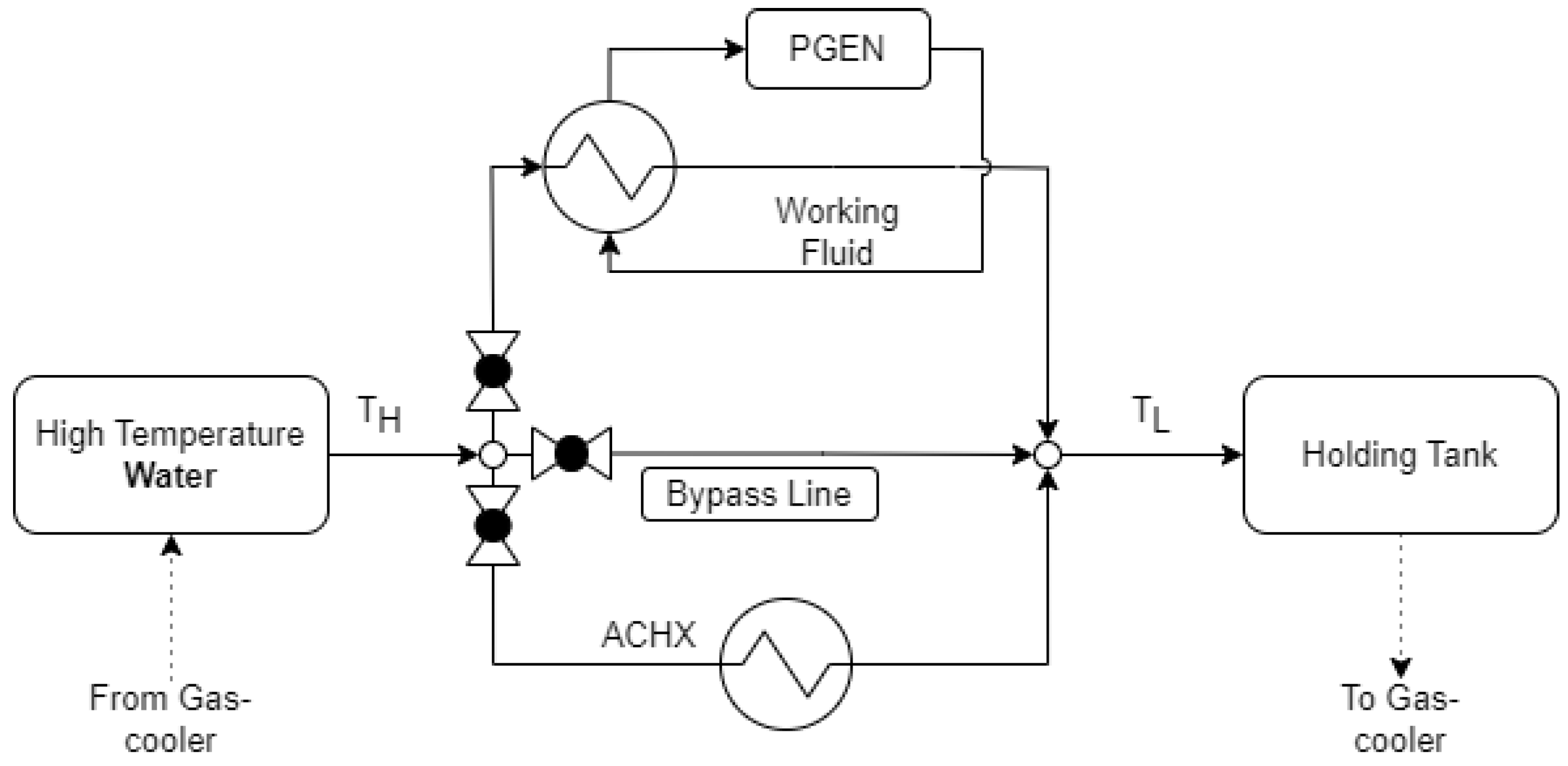
The resulting cooling cycle is displayed in Figure 1. Valves were used to designate the flow to each stream by adjusting the opening from 0 to 100%. From Figure 1, three distinct heat streams can be identified.
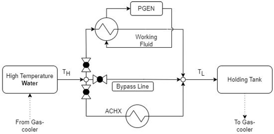
Figure 1.
Rejecting the heat from the cooling fluid.
The first heat stream flows to air-cooled heat exchangers (ACHX). In the ACHX, ambient air is used to absorb heat from the high-temperature water through forced convection.
The second heat stream flows to a power generation cycle (PGEN). In the PGEN, a working fluid is used to absorb heat from the high-temperature water. This heat is then used as the heat source in a Rankine cycle to generate electrical power.
The last heat stream is the bypass line (BP) where no heat is transferred. Therefore, this will typically be used in low-heat conditions. The water exiting the gas-cooler at a temperature near the target temperature for water entering the gas-cooler is regarded as a low-heat condition.
After the high temperature water passes through a combination of the three branches, it then enters the holding tank at a lower temperature, .
2.2. The Applicable Component and Process Limitations
To demonstrate the control philosophy, a typical production process and historical data are required. In this section, the relevant representative processes and design parameters are discussed.
The supplied design and operational parameters in this section are from an actual plant with additional information taken from the relevant literature to assign realistic parameters, where required.
The gas-cooler temperature limitations are listed in Table 1, along with the setpoint temperature of the control philosophy.

Table 1.
Process and temperature envelope values for the cooling water.
The temperature range expected for the cooling water exiting the gas-cooler is 230–280 °C, according to historical data for this specific plant. Note that the flue gas is at a significantly higher temperature. The Carnot thermal efficiency indicates that higher efficiencies can be achieved in the power generation cycle if the heat source temperature is increased. A higher temperature for the water exiting the gas-cooler can theoretically be achieved by reducing the flow rate.
However, the maximum pressure is achievable within the cooling cycle in combination with water, as the cooling fluid does not allow for higher temperature. Higher temperatures would lead to phase changes within the gas-cooler, significantly impacting the heat transfer achieved. The loss of cooling in localised areas of the gas-cooler can have potentially severe consequences.
The potential increase in thermal efficiencies, as a result of higher temperatures entering the power generation cycle, can therefore not be pursued. It also follows that the mass flow of the cooling water should not be reduced in order to increase the temperature.
The gas-cooler design and the process parameters are used to determine the operational temperature envelope for the cooling water entering the gas-cooler. The upper threshold value of 220 °C would, according to design calculations and flow rates, result in water exiting the gas-cooler below the upper temperature limit. For this system and this specific process, a lower threshold limit of 180 °C will prevent acid-dew point corrosion on the gas-cooler walls. With the objective of maximum waste heat utilisation, the target temperature is set as low as possible within the operational temperature envelope.
The individual components also have their own sets of limitations and operational ranges.
The PGEN process converts the heat to electrical power with varying thermal efficiency. The thermal efficiency is the ratio of net power generation to the total heat supplied. The efficiency can be influenced by various parameters, one of which is the heat source temperature, as shown in Figure 2.
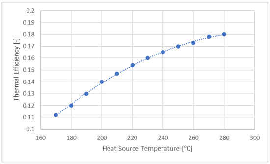
Figure 2.
Thermal efficiency of converting waste heat to electrical power as a function of heat source temperature [24] for a fixed mass flow of cooling water.
The PGEN cycle in this system is similar to that used in [24], with pentane as the selected working fluid. A thermal efficiency curve similar to that in [24] is, therefore, used to determine the power generated within the cooling process, as shown in Figure 2.
The thermal efficiency curve in Figure 2 is for a fixed mass flow of the heat source. However, since the heat source has a fluctuating temperature and flow rate profile, a varying mass flow rate is also considered in this study.
The operational limits of the PGEN system are supplied in Table 2. The maximum heat that can be assigned to the PGEN system is 100 MW. In combination with the thermal efficiency curve, the PGEN has a maximum power generation of 18 MW. According to [25], a PGEN cycle similar to the one used in this study can operate at partial load of 10%. This results in a minimum assigned heat transfer of 10 MW, which results in 1.8 MW of power generation at maximum thermal efficiency.
Table 2.
Design limitations of PGEN.
The pinch point (PP) is the minimum temperature difference between the hot and the cold stream of a heat exchanger. The minimum pinch point achievable in both the evaporator and the condenser of the PGEN is 5 °C, as used in [24].
Note that the power generation can only adjust to the heat supplied at 2%/min, in line with the study in [26]. This is only a restriction on the power generated and not on the heat transferred by PGEN, since this restriction is based on controlled turbine adjustments rather than heat exchanger limitations.
When the flow to the PGEN is such that the PGEN cannot operate within this set of limitations, a trip will occur to limit potential damage to critical process equipment, such as turbines and pumps. A trip refers to any event where the PGEN does not transfer any heat from the cooling water and, therefore, also does not generate any power.
A trip occurrence is harmful to PGEN components such as the turbine [27]. To avoid frequent trips, a time delay is typically introduced. This delay is to ensure that sufficient heat is available for a certain period of time before restarting the PGEN.
The design limits for the ACHX system are displayed in Table 3. The term ACHX refers to a network of air-cooled heat exchangers. The collective capability of the ACHX can transfer all the available heat at 100 MW.
Table 3.
Design and operational limitations of ACHX.
The thermal inertia in the heat exchanger tubes and the use of ambient air in the ACHX results in a delay for the ACHX to transfer the required heat from the distributed flow. In addition, the production plant also has a fixed rate at which the fan speed on the ACHX can be increased. This is due to an extreme scenario where the plant and the national power utility entered into an agreement regarding power demand. The failure to comply with the agreement can lead to financial penalties. As a result, the fixed rate of increasing the fan speed at the ACHX enables the plant to reduce the power demand in other processes.
Should the power demand of the production plant not be at critical levels, the only limitation on the performance adjustment is the transient response of the ACHX.
To ensure that the control formulation works as required at all times, a scenario where the production plant power consumption is at critical levels is used in this study.
In this scenario, the adjustment rate of the ACHX is constrained at 4 MW/min.
2.3. The Dataset for the Case Study
In this section, the historical dataset used to demonstrate the control philosophy is discussed.
A South African smelting plant provided a historical dataset for this study, under the condition that the values would be reworked and scaled to ensure anonymity. The gas-cooling systems in this study are applicable to various smelting operations, albeit under a different name.
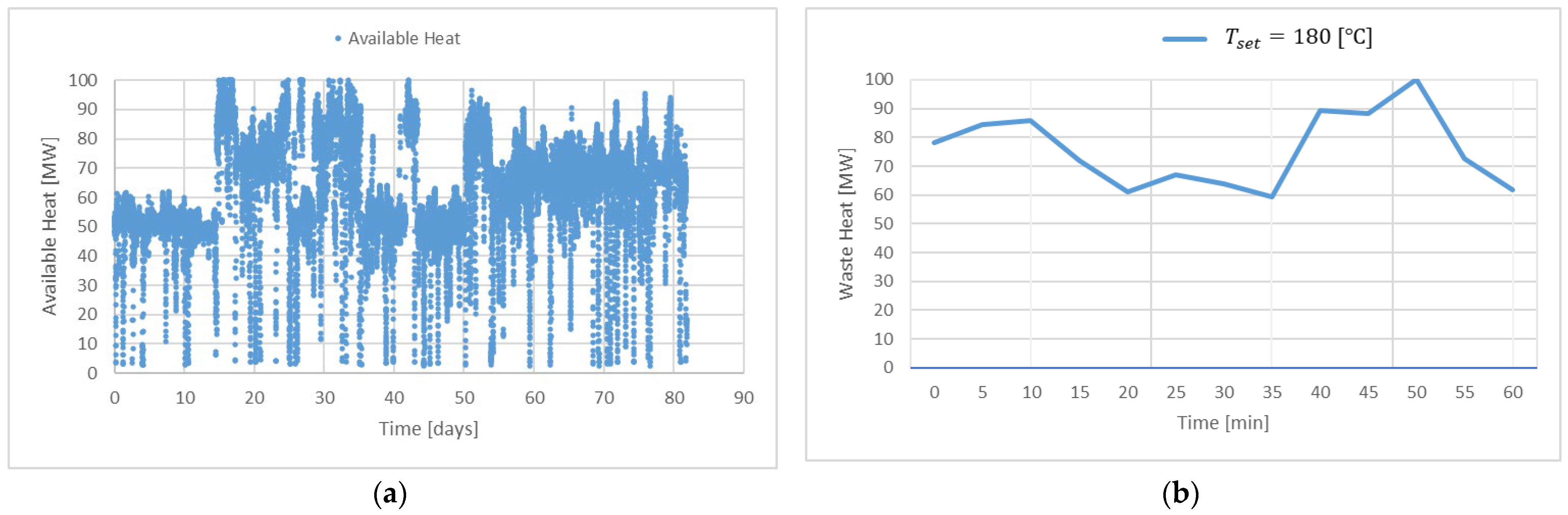
In Figure 3a, a representative waste heat profile is illustrated, consisting of 83 days of entries at 5 min intervals. From this plot, significant fluctuations over time can be observed. A demonstrative dataset ranging 60 min is used for illustrative purposes, as shown in Figure 3b. This dataset enables the demonstration of the adjustments to the flow and heat distributions between the three streams, including the influences on and the changes observed with each formulation.
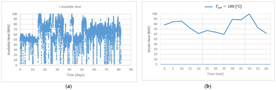
Figure 3.
(a) Representative dataset of available heat that can be transferred from the cooling fluid over 83 days. (b) Demonstrative dataset used in the demonstration.
The evaluation of power production and other performance parameters were still performed on the representative waste-heat profile in Figure 3a.
The modelling was completed within Microsoft Excel 2016 and Python 3.8, where several modules, such as NumPy 1.26.2 and Pandas 2.1.3, were used. The provided algorithms can be reproduced either within Pandas or other suitable codes.
3. The Formulation of the Control Philosophy
This section demonstrates the formulation of a control philosophy that aims to maximise power generation while ensuring that the temperature entering the gas-cooler is maintained within a suitable range when the production process is in operation.
The purpose of the control philosophy is to maximise power generation while adhering to all constraints. Unplanned stoppages of the PGEN can be used to evaluate the behaviour and the performance of the control philosophy adapting to the change in heat transfer capability. An unplanned stoppage is an unforeseen and sudden halt in the normal operation of a process that causes disruptions and potential production delays. For PGEN, this results in a loss in heat transfer capacity and power generation.
An unplanned stoppage is introduced in the use of both datasets in Figure 3. The average mean time between failures (MBTF) for the PGEN used in this study indicates that no more than one unplanned event can be introduced for both profiles. This is in agreement with the literature of [28]. Trips due to low heat availability are also included, as is discussed in the formulations below.
The importance of the heat rejection process in the main production process has been described in detail in previous sections. The flue gas leaving the gas-cooler needs to be within the safe operational temperature envelope. This is achieved by controlling the temperature of the cooling water entering the gas-cooler, referred to as . A loss in the heat rejection capacity of the cooling system can potentially cause the cooling water temperature to move outside the operational envelope. This increases the risk of disruptions to the production process.
The gas-cooler operation adjusts the mass flow rate of the water depending on the temperature entering the gas cooler to ensure that a sufficient heat transfer is maintained. The mass flow of the cooling water, therefore, inherently considers the current gas-cooler heat transfer efficiency. The mass flow and temperature of the cooling water can thus be used alongside a target temperature to determine the available waste heat.
3.1. A Typical Works Philosophy
A typical works philosophy is proposed as a baseline. In this philosophy, the heat and flow distributions are fixed between all heat exchangers.
The control philosophy is described using binary operators and condition statements. Therefore, this section first describes all relevant parameters and the writing conventions and symbols used for each.
The conservation equation for energy, reproduced from [6], is:
where is the change in energy for the control volume, while and are the energy flowing into and out the control volume. Since heat is either transferred out of the control volume through the PGEN or the ACHX, Equation (2) can be rewritten as:
where is the total available heat and , , and are the heat in MW distributed to the PGEN, ACHX, and bypass, respectively. Failing to remove between the PGEN and ACHX components will result in residual heat, where . This heat term is an indication of the difference between the temperature exiting the heat rejection cycle, [°C], and the target temperature set out in Table 1. The exit temperature can be calculated as:
where and are the mass flow rate and specific heat of the cooling water. It follows that, in a scenario where sufficient heat transfer is performed, , and, therefore, .
The time index for the formulation is given by . The cooling water enters the heat rejection cycle at a temperature of [°C] and a mass flow rate of [kg/s]. At time , a process model uses the desired temperature of the cooling water entering the gas-cooler, [°C], to determine the heat to be transferred, [MW].
A binary parameter, , is introduced, where a non-zero value indicates that the power generation process is operational and available to transfer heat. A value of zero indicates that the power generation cycle is not available.
To prevent frequent trips to the PGEN in low heat conditions, a time delay is introduced for a PGEN currently offline. This ensures that the PGEN does not start until periods have passed, where sufficient heat is available. Other reasons for a stoppage will externally force the value of to be zero until rectified.
The heat assigned to the PGEN, , must be more than the lower limit, [MW], of the power-generating process. The process control within PGEN will adjust working pressures and the mass flow rates of the refrigerant to transfer the required heat, within the constraints of the PGEN design. The PGEN component converts to electrical power at a heat source temperature-dependent thermal efficiency, as shown in Figure 2.
It follows that a higher value for results in a higher power generation. It can also be argued from (3) that a higher value results in a higher for the cooling water entering the gas-cooler. The formulations to follow, therefore, attempt to minimise while also attempting to maximise .
Any heat not transferred by the PGEN needs to be assigned to the ACHX. The heat distributed to ACHX is [MW]. Due to the use of a fan and ambient air to transfer heat, the heat transfer rate increase is limited at . Note that ACHX can consist of multiple air-cooled heat exchanger units. The distribution of heat and mass flows between the individual units does not fall within the scope of this study. Therefore, the ACHX is treated as a single system with a relatively wide operational range.
For the typical works philosophy, a parameter, [-], is introduced that represents the share of heat distributed to the PGEN. This parameter is predetermined and fixed, independent of heat source parameters.
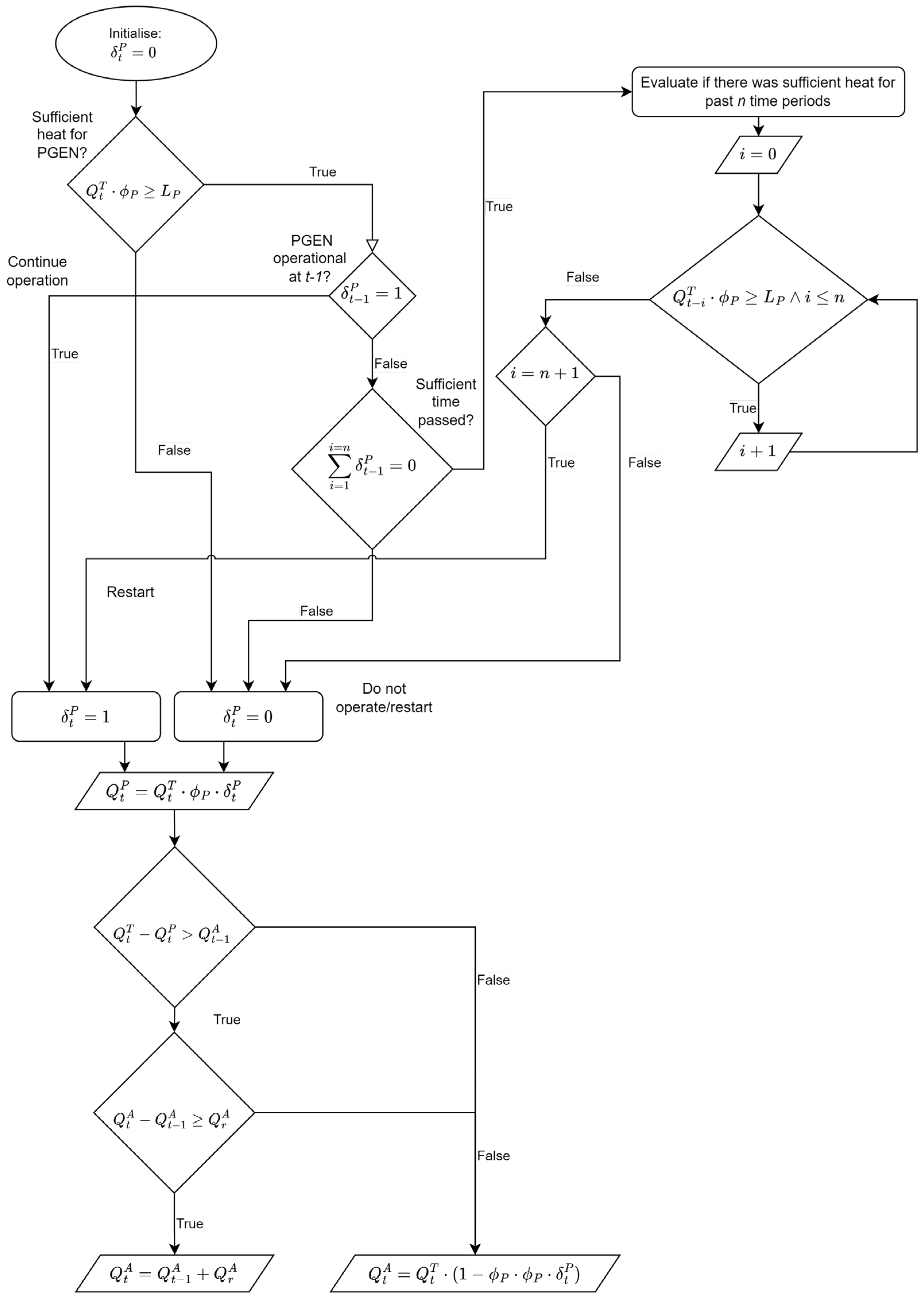
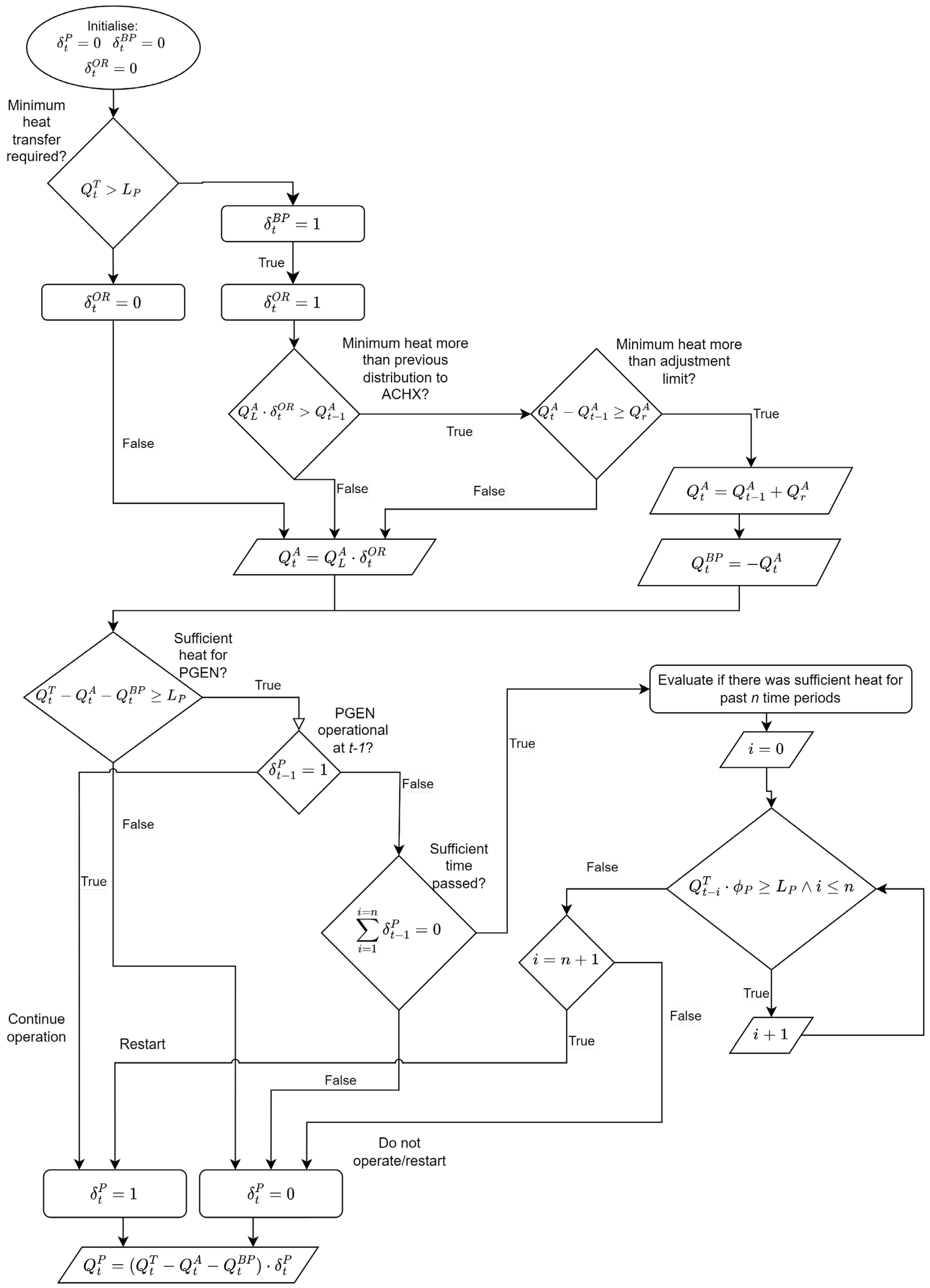
The heat distributions to the ACHX, PGEN, and BP at time are determined through the algorithm illustrated in Figure 4.
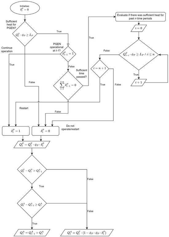
Figure 4.
Block diagram for Algorithm 1 (WPLC).
To demonstrate the behaviour of the control formulations, the plant parameters set out in Table 2 and Table 3 will be used, with additional parameters being supplied where required. The setpoint temperature , as in Table 1. The PGEN has a lower heat limit of MW. The heat of is converted to power according to the curve in Figure 2. The ACHX can only increase its heat transfer capability by 4 MW/min. The time period of the sufficient heat required before a restart is 15 min; . The formulation will be applied to the demonstrative dataset in Figure 3b.
3.1.1. The Results of WPLC on the Demonstrative Dataset
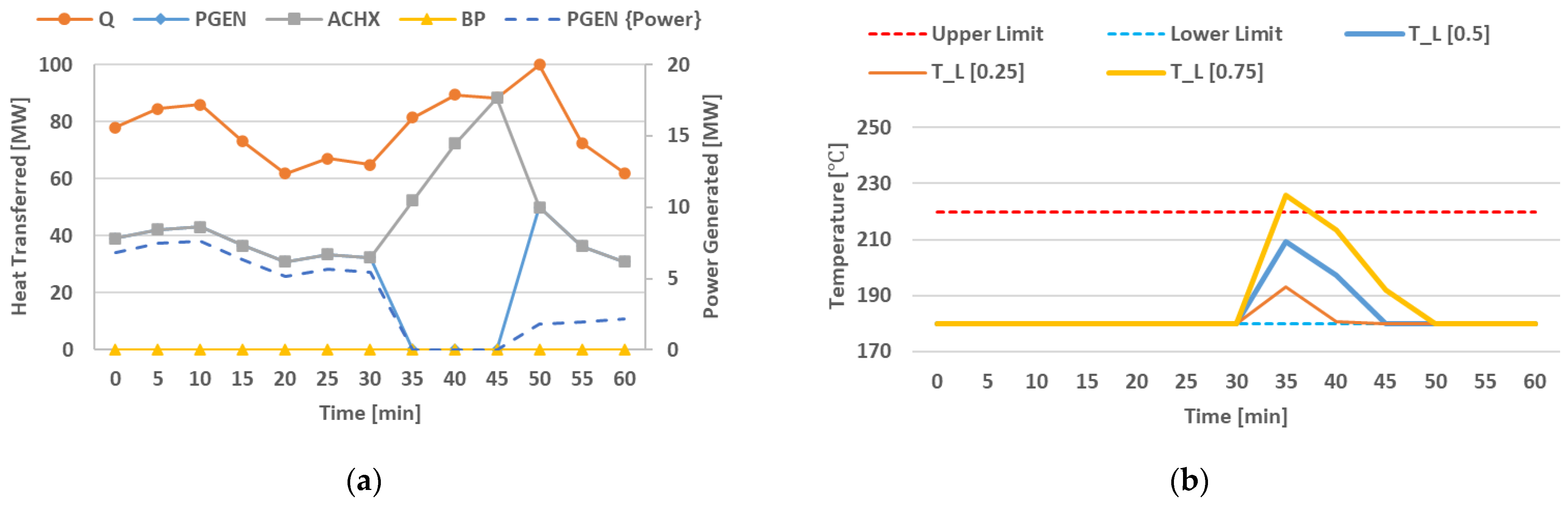
In Figure 5a, the heat distribution between the components based on the demonstrative dataset (Figure 3b) is illustrated.
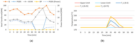
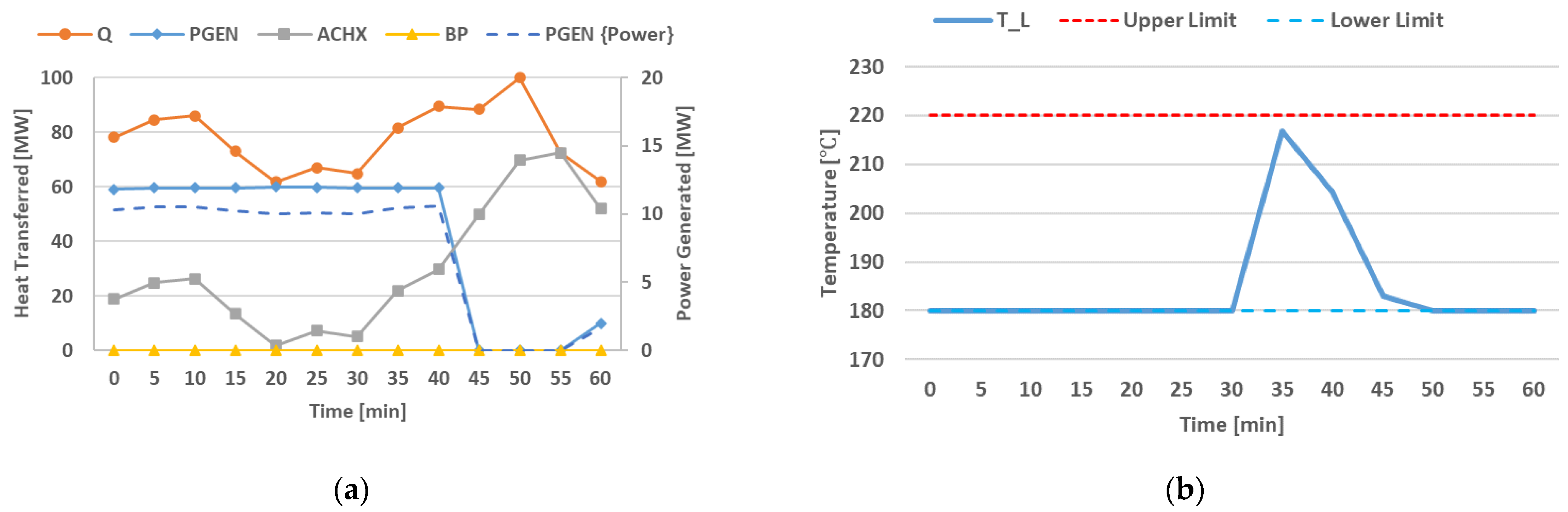
Figure 5.
(a) Heat distribution between the PGEN, ACHX, and BP over time for WPLC. An overlay of the available heat (Q) is included. (b) Illustration of temperature entering the gas-cooler over time for WPLC, with = 0.5 as well as = 0.25 and 0.75.
The fixed ratio of heat distribution between components are notable, with both components following the curve of the waste heat, with the exception of 35–45 min, where the PGEN was unavailable due to an unplanned event. It is also noted that during time periods where PGEN was unavailable, the ACHX attempted to transfer as much of the waste heat as possible within its adjustment constraint. Note that the power generation after the PGEN restarted was at the lower limit and only increased by the 2 %/min, while the heat transferred by the PGEN did not follow this restriction.
The value of over the same time span is shown in Figure 5b. The unplanned unavailability of the PGEN results in the ACHX needing to transfer all the required heat. However, since the ACHX can only realistically increase the heat transfer by 4 MW/min, the required heat transfer cannot be instantaneously satisfied by the ACHX. It follows that this scenario will result in , and from (3), it follows that .
The results in the demonstrative dataset indicate clearly that the conservation principles given in Equation (2) are adhered to, with temperature increases noted where .
The value of can be adjusted in an attempt to maximise power generation. The value of remains within the temperature envelope even with the unplanned availability of the PGEN, as shown in Figure 5b. The ACHX is able to adjust quickly enough to transfer the heat that would have been distributed to the PGEN.
This can indicate that the fixed ratio is too conservative and that more heat can be distributed to the PGEN to increase the power generated by the system. Using the same formulation, the value of is adjusted to a more aggressive approach, where .
The temperature curve for with this approach indicates that the temperature moved outside the operational envelope. This was due to the ACHX receiving only 25% of the heat before needing to adjust to transfer 100% of the heat. This approach can, therefore, be seen as too aggressive, given the supplied demonstrative dataset.
The opposite can also be shown for the more conservative approach, where results in only a small increase in when the PGEN becomes unavailable. This is due to the ACHX initially receiving 75% of the heat before having to adjust to transfer 100% of the heat.
It is concluded that a conservative value for will not result in maximum power generation but will have reduced risk, whereas an aggressive value will deliver more power generation but with increased risk of breaching the temperature envelope.
The above results are only for a demonstrative dataset to illustrate the effect of changes made to parameters. In the next section, the formulation will be applied to the historical dataset shown in Figure 3a.
3.1.2. The Results of WPLC on the Historical Dataset
The WPLC is applied to the larger dataset for four different values. The value of is changed from 0.1 to 0.9 to determine the ideal ratio for the specific heat profile shown in Figure 3a. An unplanned stoppage is also forced on three different time periods to evaluate the influence of heat source properties on the preferred value of .
It has been indicated in the previous section that a higher value for will result in a higher heat distribution to the PGEN. This indicates that more power will be generated. The value of is, therefore, varied between 0.5 and 0.8 to determine the highest value that is still conservative enough to ensure adequate cooling in the event of an unplanned trip. Unplanned events 1, 2, and 3 take place at 8.5, 24.75 and 32.6 days into the timeline of the historical dataset.
Since the objective of this study is to maximise power generation whilst keeping within the operational temperature envelope, the maximum value for needs to be identified where the is still within the operational envelope.
This value is indicated with a shaded column in Table 4. A value of 0.7 for causes the cooling water to move out of the operational temperature envelope for only one of the unplanned events. This indicates that the impact that the distribution ratio has is dependent on the heat source parameters at the time of the unplanned event.
Table 4.
Results for heat rejection cycle for a range of and unplanned events.
A value of 0.6 for is thus identified as the desired setting, which delivers adequate cooling at all times, while also being conservative enough that the highest value for after an unplanned trip is inside the envelope at 213.8 °C.
The impact of on the power generation is supplied in Table 5 along with more aggressive and conservative values. Evaluating the average power generation along with the maximum temperatures indicates that the more conservative value for delivers a lower temperature and lower power generation. This is due to a significant share of heat being distributed to the ACHX to ensure that it can readily adjust to transfer if the PGEN were to become unavailable.
Table 5.
Results for heat rejection cycle for a .
The opposite is also true; the more aggressive value delivers a higher average power generation as well as a value for that breaches the temperature envelope. This is due to the PGEN receiving a larger share of the heat, resulting in ACHX having to increase over a longer time to meet the heat transfer requirement in case of an unplanned event.
This results section shows that a fixed value for the distribution ratio is not the desired approach for a fluctuation in the heat source.
The results and discussions above conclude that the ratio of distribution should be dependent on the parameters of the heat source at any given time. It follows that the ratio of distribution needs to be continuously adjusted.
3.2. The Ongoing Readiness of the ACHX
The WPLC is a typical works philosophy where the heat is distributed at a fixed ratio between the PGEN and the ACHX. The WPLC shows that a fixed ratio of heat distribution between the PGEN and the ACHX is not ideal due to the potential of unplanned stoppages.
This section formulates a control algorithm that ensures an adequate heat transfer is maintained at all times by continuously being ready for an unplanned stoppage. This will be achieved by calculating and distributing a share of the heat to the ACHX that mitigates any risk of temperatures outside the operational envelope for the gas-cooler.
For this purpose, a binary parameter, , is introduced. A value of one indicates that the control philosophy must anticipate an unplanned stoppage every time period. To determine the value of , a minimum heat transfer, [MW], is firstly calculated. Determining is carried out through Equation (4) below:
where is the upper temperature limit of the operational temperature envelope. Note that if , the term will be negative, and that is set to zero. In this scenario, all the heat can be assigned to the PGEN for power generation without risk, since failing to transfer any heat will only result in and thus .
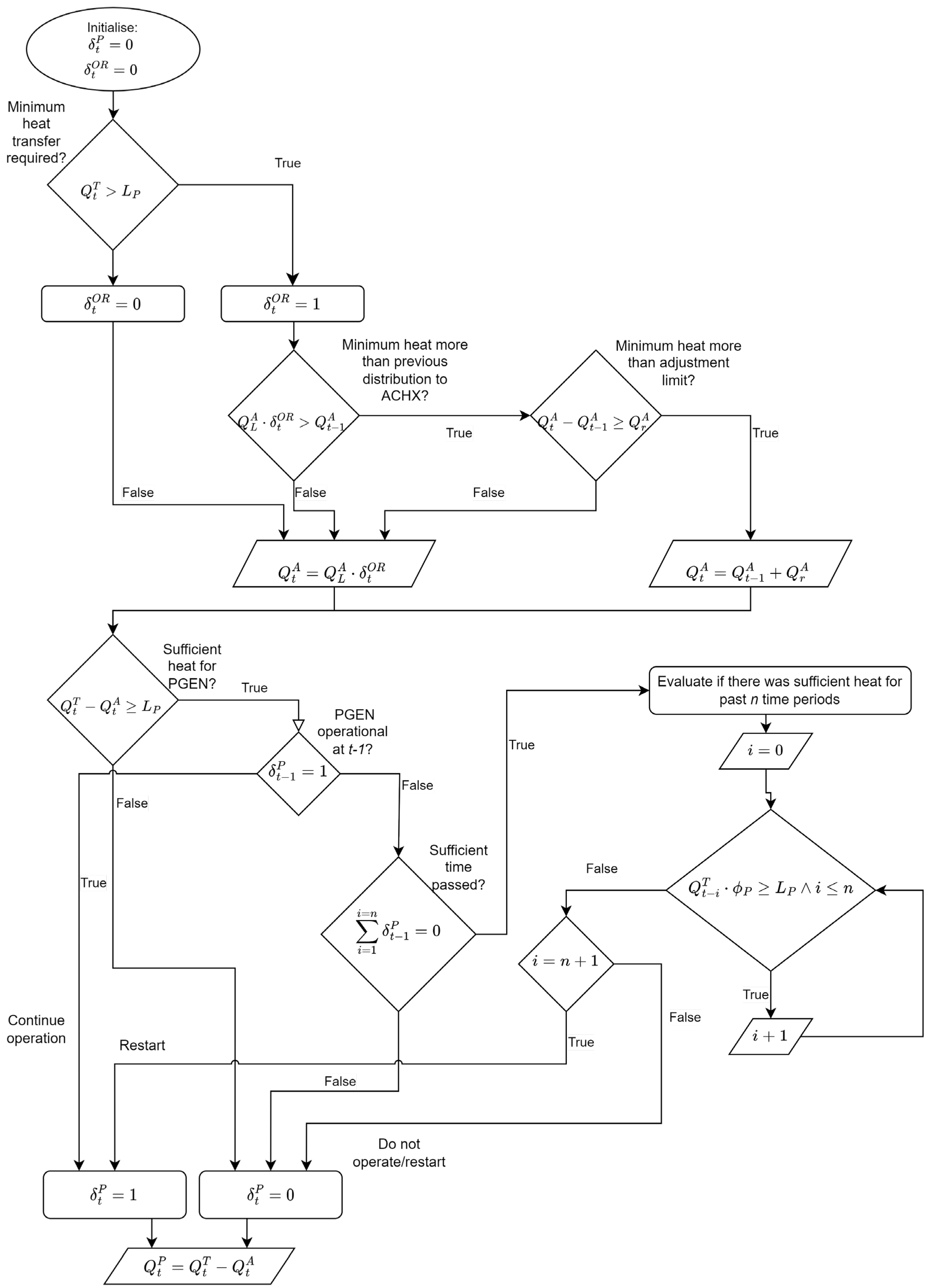
The heat distribution between the PGEN and the ACHX is determined through the algorithm illustrated in Figure 6.

Figure 6.
Block diagram for Algorithm 2 (ORLC).
To demonstrate the behaviour of the ORLC, the same plant parameters set out in Section 3.1 are used. In addition, the upper temperature limit for the operational envelope, , is used, as noted in Table 1.
3.2.1. The Results of the Continuous Readiness of the ACHX on the Historical Dataset
The results of applying this formulation to the demonstrative dataset in Figure 3b is shown in Figure 7a,b.
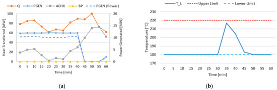
Figure 7.
(a) Heat distribution between the PGEN, ACHX, and BP over time for the formulation in Section 3.2. An overlay of the available heat (Q) is included. (b) Illustration of temperature entering the gas-cooler over time for the formulation in Section 3.2.
The first significant difference noted in Figure 7 is in the heat transferred by the PGEN and the ACHX. Previously, these curves followed the same values, whereas, in this formulation, they differ. The fluctuation of results in a varying value of . This is due to the difference between and being used in its calculation. Note that this results in a constant value for . It can be argued that the heat transfer assigned to the ACHX reduces the cooling water to the upper temperature limit, , whereas the PGEN then transfers the residual heat contained between and .
Through the comparison of Figure 5 and Figure 7, the heat distributed to the PGEN clearly has lower fluctuations for the ORLC compared to the WPLC. By comparing the resulting power generation, as is done in Figure 8, it can be noted that the PGEN with the WPLC observed higher power generation figures for only 10 min of the 60 min range. It is expected that the ORLC will result in an increase in power generation on the demonstrative dataset. This is dependent on the signature waste-heat profile and will need to be evaluated in the historical dataset for an accurate conclusion.
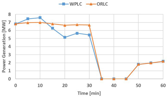
Figure 8.
Power generation comparison between ORLC and WPLC.
3.2.2. The Results of the Continuous Readiness of the ACHX on the Historical Dataset
The control philosophy given above can be demonstrated on the historical set of data illustrated in Figure 3a. The results are summarised in Table 6.
Table 6.
Results for heat rejection cycle for ORLC.
It is noted that the power generation increased from an average of 6.11 MW to 6.41 MW with this philosophy. The maximum power generation, however, reduced from 10.4 MW to 9.61 MW. The maximum temperature for reduced from 217.1 to 204.5 °C, which indicates that the current formulation is a definite improvement of the typical works philosophy.
This formulation is definitely successful in its objective to adjust the distribution between the ACHX and the PGEN to the extent that a sufficient heat transfer can be guaranteed at all times.
3.3. Advanced Bypass Utilisation
In ORLC, it is noted that did not exceed any of the temperature limits for any given period. By ensuring that the heat transfer demand is always met, additions to the control formulation can now be made in an attempt to maximise power generation.
To increase the observed power generation, a binary parameter, , is introduced. A non-zero value indicates that the control philosophy will make use of the bypass line to maintain a desirable value for while assigning as much heat transfer to the PGEN process as possible. The conservation of energy and mass in (2) and (3) will still hold, with the heat and mass flows assigned to the bypass compensating for the higher heat transfer rate achieved in the PGEN.
When , the value of the minimum heat assigned to the ACHX, , is also bypassed. If successful, it follows from Equation (1) that a larger is observed in comparison to the previous section.
The heat distribution to the ACHX, PGEN and BP streams are determined through the algorithm illustrated in Figure 9.

Figure 9.
Block diagram for Algorithm 3 (ABLC).
3.3.1. The Results of the Advanced Use of Bypass on the Demonstrative Dataset
Figure 10 can be compared to Figure 5 and Figure 7. A significant difference is the consistent use and adjustment of flow in the BP. This allows the ACHX to maintain the minimum required heat transfer while allowing the PGEN to operate at maximum capacity whenever possible. This can be confirmed through the evaluation of the power generated being significantly higher than for previous formulations.
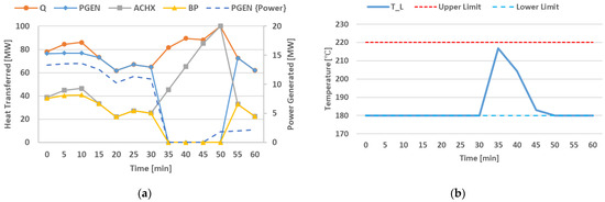
Figure 10.
(a) Heat distribution among PGEN, ACHX, and BP over time for the formulation described in Section 3.3. Overlay of the available heat is included. (b) Illustration of temperature entering the gas-cooler over time for the formulation in Section 3.3.
The power generation performance between WPLC, ORLC, and ABLC are illustrated in Figure 11. The control formulation in ABLC shows an increase in the heat distributed to the PGEN and it is, therefore, expected that the ABLC will result in an increase in observed power generation. Figure 10 and Figure 11 shows that ABLC includes all operational constraints and limitations as required.
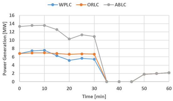
Figure 11.
Power generation comparison between ORLC, WPLC and ABLC (demonstrative data).
The formulation of ABLC is, therefore, suitable to be tested on the historical dataset.
3.3.2. The Results of Advanced Use of Bypass on Historical Dataset
The formulation in Section 3.3 is now applied to the historical dataset in Figure 3a. The results are summarised in Table 7.
Table 7.
Results for heat rejection cycle for ABLC.
A significant increase in average and maximum power generation are noted. The average power generation increased by 57.8% from 6.41 MW to 10.12 MW. This is achieved without any increase in the value for , indicating that there is no added risk to this formulation in terms of moving outside the operational temperature envelope.
From the above results, it is clear that the formulation of ABLC is successful in significantly increasing the power generation by PGEN. This is achieved while still ensuring that ACHX is always ready to transfer all the required heat at a rate fast enough that there is no risk of moving outside the temperature envelope, even in case of an unplanned trip.
3.4. The Use of Predictive Parameters
The ABLC was successful in significantly increasing the power produced whilst still ensuring that stayed within the desired temperature envelope at all times.
From historical plant data and process models, future heat transfer requirements can be predicted with a level of certainty. This may allow adjustments to the heat distribution to further improve on power generation without adding risk.
Plant operational models and historical datasets can be used to determine the feedforward parameters that indicate whether an increase in available heat can be expected in the following periods.
It is noted in Table 1 and discussed in Section 2 that the PGEN has a limit on how fast the power generation can be adjusted. It is also noted that this constraint originates from turbine control and not from the heat exchanger’s capability. From this, it can be argued that increasing the heat transferred to the PGEN before a significant increase is observed in can result in the PGEN increasing the power generation without adding significant risk. By increasing the power generation earlier, the PGEN will have smaller adjustments to make once a significant increase in is observed.
From historical datasets, certain process procedures can be identified that lead to a required relative heat transfer increase in in the next time periods. A binary parameter, , is introduced, where a non-zero value indicates that . If an increase in heat is expected, then the heat transfer required from the PGEN will either be the maximum operational limit or a product of with its previous value, .
Since the philosophy of ORLC is still present in this formulation, the value of needs to be limited to ensure that the ACHX can still meet the heat transfer requirements in case the PGEN becomes unavailable.
This ensures that the operational limits of all components are adhered to, while maintaining a safe value for .
Note that the ACHX minimum heat distribution, , is still assigned. Therefore, this philosophy can potentially lead to assigning more heat transfer requirements to the ACHX and PGEN than is required at time . It follows that the bypass must be used to maintain the temperature above the lower limit, according to Equation (1). Therefore, this control philosophy only allows the use of predictive parameters to maximise power generation if the value of is also a non-zero value.
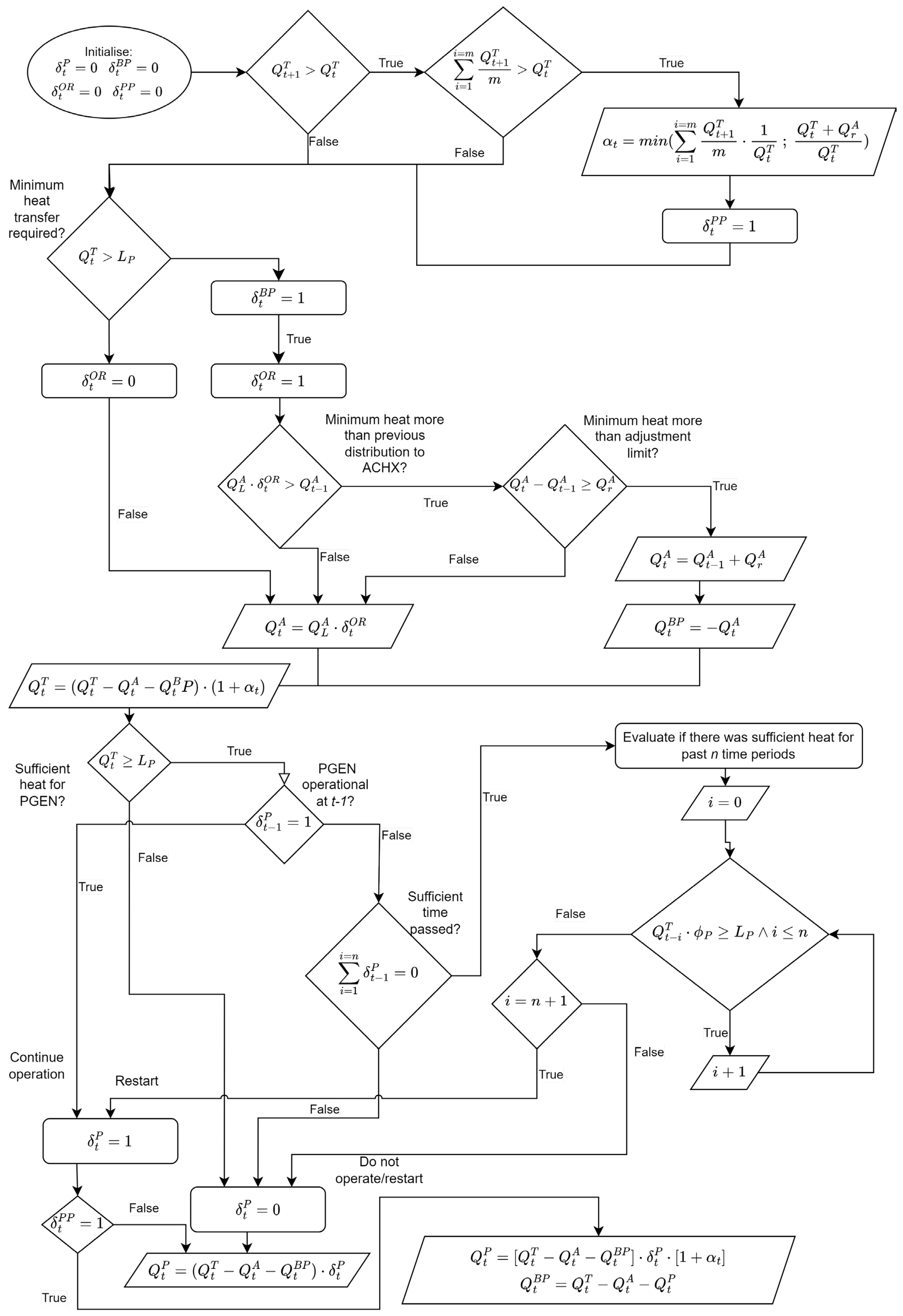
The heat distribution between the PGEN, ACHX, and BP are determined through the algorithm illustrated in Figure 12.
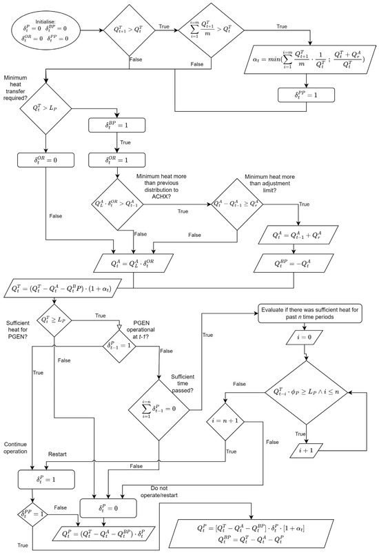
Figure 12.
Block diagram for Algorithm 4 (PPLC).
3.4.1. The Results of Using Predictive Parameters on the Demonstrative Dataset
Figure 13 can be compared to Figure 5, Figure 6 and Figure 10. A minor increase in the heat distributed to the PGEN is noted. To ensure , the BP is also increased slightly to prevent breaching the temperature envelope on the lower limit. No changes are noted in the heat distribution to the ACHX.
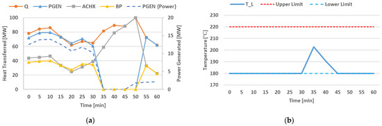
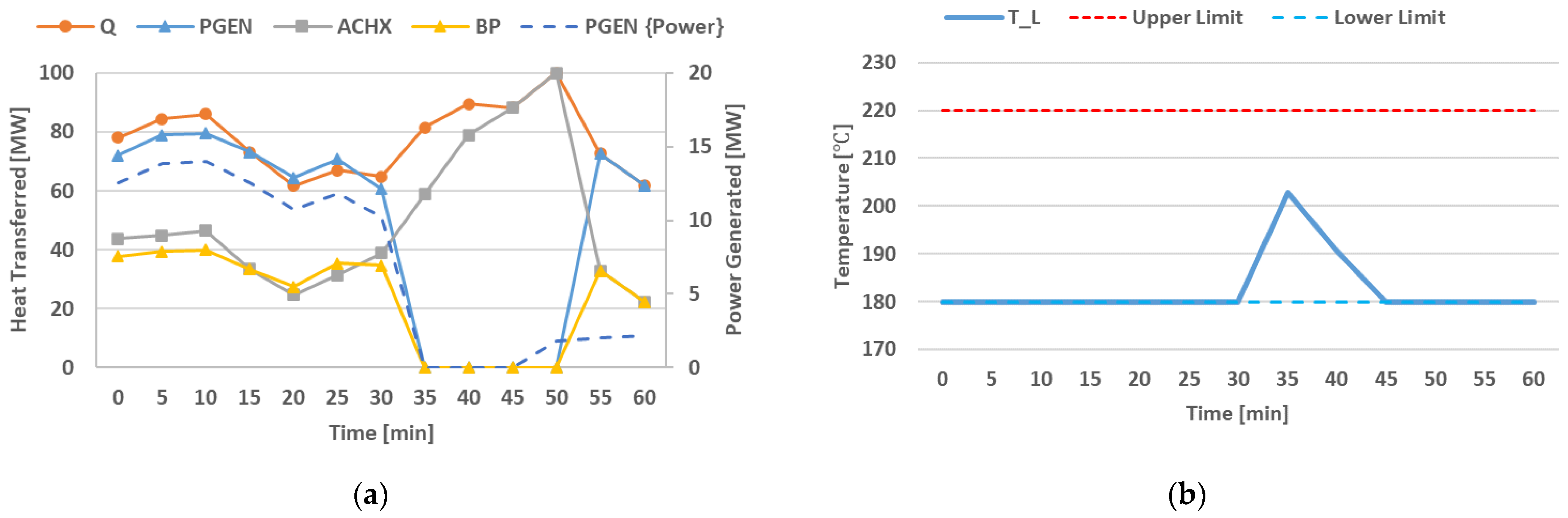
Figure 13.
(a) Heat distribution among PGEN, ACHX, and BP over time for the formulation described in Section 3.4. Overlay of the available heat is included. (b) Illustration of temperature entering the gas-cooler over time for the formulation in Section 3.4.
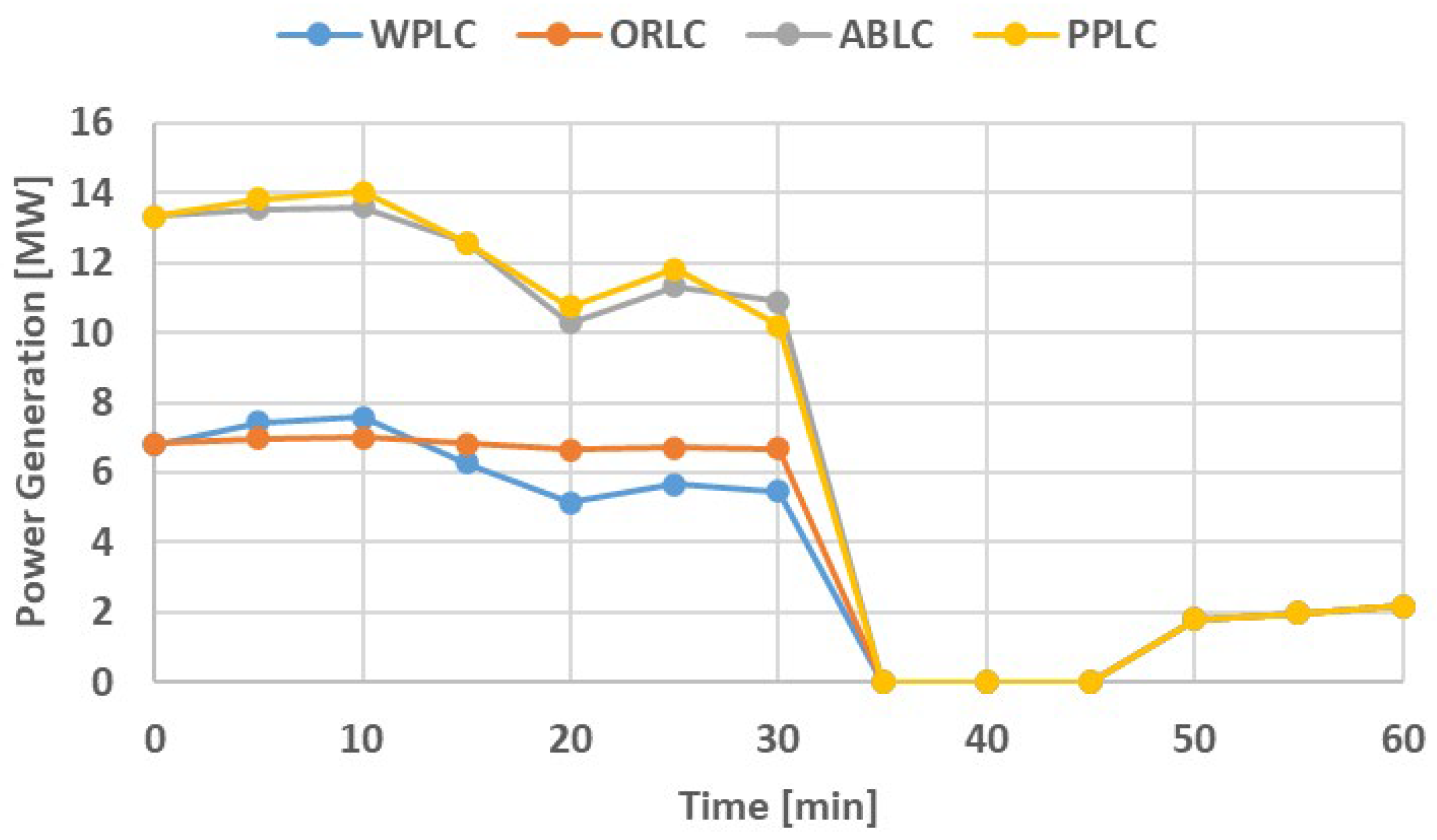
The power generation performances of WPLC, ORLC, ABLC, and PPLC are illustrated in Figure 14. Note that the slight increase in heat distribution to PGEN has resulted in a small increase in power generation compared to the previous formulation of ABLC.

Figure 14.
Power generation comparison between WPLC, ORLC, ABLC and PPLC for the demonstrative dataset.
Figure 12 and Figure 13 show that PPLC includes all operational constraints and limitations as required, and is working as required and expected.
The formulation of PPLC is therefore suitable to be tested on the historical dataset.
3.4.2. The Results of Using Predictive Parameters on the Historical Dataset
The formulation is applied to the historical dataset of Figure 3a with the results summarised in Table 8.
Table 8.
Results for heat rejection cycle for PPLC.
The average power generation increased by 5.5% from 10.12 MW to 10.68 MW. The maximum values observed for indicate minimal added risk. The unplanned event is triggered in a time period where . As noted in Section 3.4.1, the flow through the bypass increased. However, no change in maximum temperature is noted. This is due to the value of being influenced by the adjustment capability of the ACHX every time.
4. Conclusions
The formulation of a control philosophy for the heat rejection process was demonstrated. The main priority of the control philosophy is to ensure that the heat rejection process transfers sufficient heat from the cooling fluid to other components or processes. This ensures that the temperature of the cooling fluid entering the gas-cooler remains within the required range. A failure to do so can result in production interruptions that can be associated with significant losses for the plant owner. In addition, the availability of a power generation cycle also makes waste-heat recovery and power generation a priority.
Therefore, the control philosophy needs to calculate both the heat and mass flow distributions between the ACHX, PGEN, and BP. The control algorithm also needs to adjust to changes in the received flow from time to .
Note that all control formulations in this study consider a scenario where the power consumption of the plant is at critical levels. As discussed, this results in the need to constrain the ramp-up rate of the ACHX. The results of the control formulations shown in this study are for the most extreme scenario to ensure that the control formulations perform as required at all times. Should power consumption not be near critical levels, only a transient response will constrain the heat transfer adjustment of the ACHX.
The formulation starts with a typical works control philosophy. In this formulation, the distribution of heat between the ACHX and PGEN is fixed, independent of the fluctuating heat source. Based on the historical data, a suitable ratio is selected that satisfies the heat transfer requirement, even in the event of an unplanned trip of the PGEN. It is shown that the ratio of distributions needs to adjust according to the heat source parameters to ensure maximum power generation without any added risk of moving out of the temperature envelope.
This is rectified with the next formulation, where the minimum heat is always assigned to the ACHX with the residual heat then distributed to the PGEN. This resulted in the temperature remaining within the operational limits, but with an improvement in power generation. An average power generation of 6.41 MW was observed.
The advanced use of BP ensures that is maintained within the desired temperature envelope while also allowing the PGEN to transfer significantly more heat than previously allowed. This significantly improved the average power generation to 10.12 MW.
The addition of feedforward parameters to predict the increase in available heat increased the average power generation by another 5.5%, resulting in an average of 10.68 MW.
Through the formulation process, the control algorithms are simulated on a demonstrative dataset for evaluation to ensure the scientific soundness of the results once applied to the larger historical dataset. All evaluations have shown that the WPLC, ORLC, ABLC, and PPLC work as intended. The limitations of components are never breached, and adjustments are always made within the capability of each component. The changes in formulations also deliver the expected changes in heat distribution between the components.
The formulated control philosophy successfully maximised energy recovery while ensuring that the temperature was maintained in the desired temperature envelope.
The novel contributions of this paper are the three control philosophies that consider the stochastic effect of a fluctuating heat source. These formulations then successfully distribute the waste heat between the ACHX, PGEN, and BP in such a way that maximises energy recovery without any risk to the production process, even with a sudden loss in heat transfer capabilities such as an unplanned trip event for the PGEN.
A potential future study could include the formulation of a control philosophy for an ACHX that consists of multiple heat exchangers, where each individual heat exchanger has different design parameters. The formulation can then attempt to ensure a maximum heat transfer for a minimum power input to forced convection equipment. An additional study could be carried out to increase the fidelity of the PGEN component. The internal control of the PGEN can lead to an improved conversion ratio of the power generated to the heat transfer.
Author Contributions
Conceptualisation, J.P.B., M.V.E. and P.v.Z.V.; Formal analysis, J.P.B. and P.v.Z.V.; Investigation, J.P.B., M.V.E. and P.v.Z.V.; Methodology, J.P.B., M.V.E. and P.v.Z.V.; Validation, J.P.B. and P.v.Z.V.; Visualisation, J.P.B. and P.v.Z.V.; Writing—original draft, J.P.B.; Writing—review and editing, M.V.E. and P.v.Z.V. All authors have read and agreed to the published version of the manuscript.
Funding
This research received no external funding.
Data Availability Statement
Data are contained within the article. Historical dataset not publicly available due to NDA with data provider.
Conflicts of Interest
The authors declare no conflict of interest.
Nomenclature
| Greek Letters | |||
| Specific heat of Fluid, | Thermal efficiency | ||
| Density, | |||
| Temperature, | Expected relative increase in | ||
| Mass flow rate | Fixed distribution ratio to PGEN | ||
| Binary decision variable for ABLC | |||
| Heat Streams | Binary decision variable for PPLC | ||
| Waste heat stream, | Binary decision variable for ORLC | ||
| Heat distributed to PGEN, | Binary decision variable for PGEN availability | ||
| Minimum heat distributed to ACHX, | Subscripts | ||
| Heat distributed to ACHX, | Hot fluid | ||
| Heat distributed to Bypass, | Wall of heat exchanger | ||
| Limits/Setpoints | Outlet | ||
| Heat Adjustment Limit for ACHX, | Cold fluid | ||
| Upper temperature for envelope, | Inlet | ||
| Setpoint temperature, | Maximum | ||
| Lower operational limit of PGEN | Minimum | ||
| Residual | |||
References
- Gupta, R. Chapter 4.2—Energy Resources, Its Role and Use in Metallurgical Industries. In Treatise on Process Metallurgy; Industrial Processes, Part A; Elsevier: Amsterdam, The Netherlands, 2014; Volume 3, pp. 1425–1458. [Google Scholar]
- Jalkanen, H.; Holappa, L. Chapter 1.4—Converter Steelmaking. In Treatise on Process Metallurgy; Industrial Processes, Part A; Elsevier: Amsterdam, The Netherlands, 2014; Volume 3, pp. 223–270. [Google Scholar]
- Wang, B.; Zhou, J.-A.; Xie, J.-B.; Liu, Z.-Q.; Zhang, H.; Zhou, L.-H. Numerical and Experimental Investigations of Converter Gas Improvement inside a Flue Using Its Waste Heat and CO2 by Pulverized Coal Injection. Environ. Prog. Sustain. Energy 2018, 37, 1503–1512. [Google Scholar] [CrossRef]
- Hosseini, R.K.; Yareiee, S. Failure analysis of boiler tube at a petrochemical plant. Eng. Fail. Anal. 2019, 106, 104146. [Google Scholar] [CrossRef]
- Hemadri, V.B.; Subbarao, P. Thermal integration of reheated organic Rankince cycle (RH-ORC) with gas turbine exhaust for maximum power recovery. Therm. Sci. Eng. Prog. 2021, 23, 100876. [Google Scholar] [CrossRef]
- Incropera, F.P.; DeWitt, D.P.; Bergman, T.L.; Lavine, A.S. Fundamentals of Heat and Mass Transfer; John Wiley & Sons: Hoboken, NJ, USA, 2007. [Google Scholar]
- Ravi, R.; Pachamuthu, S.; Shivaprasaf, K.; Kasinathan, P.; Anandan, S.; Sundarababu, J. CFD analysis of innovative protracted finned counter flow heat exchanger for diesel enginer exhaust waste heat recovery. AIP Conf. Proc. 2021, 2316, 030024. [Google Scholar]
- Jiménez-Arreola, M.; Pili, R.; Margo, F.D.; Wieland, C.; Rajoo, S.; Romagnoli, A. Thermal power fluctuations in waste heat to power systems: An overview on the challenges and current solutions. Appl. Therm. Eng. 2018, 134, 576–584. [Google Scholar] [CrossRef]
- Inayat, A. Current progress of process integration for waste heat recovery in steel and iron industries. Fuel 2023, 338, 127237. [Google Scholar] [CrossRef]
- Parra-Camacho, L.; Rodriguez-Bayona, A.; Carreno-Zagarra, J. Automation and control of the thermal mixing process. Syst. Sci. Control Eng. 2023, 11, 2177769. [Google Scholar] [CrossRef]
- Li, X.; Xu, B.; Tian, H.; Shu, G. Towards a novel holistic design of organic Rankine cycle (ORC) systems operating under heat source fluctuations and intermittency. Renew. Sustain. Energy Rev. 2021, 147, 111207. [Google Scholar] [CrossRef]
- Zhao, R.; Zhang, H.; Song, S.; Tian, Y.; Yang, Y.; Liu, Y. Integrated simulation and control strategy of the diesel engine–organic Rankine cycle (ORC) combined system. Energy Convers. Manag. 2018, 156, 639–654. [Google Scholar] [CrossRef]
- Shu, G.; Li, X.; Tian, H.; Shi, L.; Wang, X.; Yu, G. Design condition and operating strategy analysis of CO2 transcritical waste heat recovery system for engine with variable operating conditions. Energy Convers. Manag. 2017, 142, 188–199. [Google Scholar] [CrossRef]
- Yebi, A.; Xu, B.; Liu, X.; Shutty, J.; Anschel, P.; Onori, S.; Filipi, Z.; Hoffman, M. Nonlinear model predictive control strategies for a parallel evaporator diesel engine waste heat recovery system. In Proceedings of the ASME 2016 Dynamic Systems and Control Conference, Minneapolis, MN, USA, 12–14 October 2016. [Google Scholar]
- Ponce, C.; Sáez, D.; Bordons, C.; Bordons, C.; Nú, A. Dynamic simulator and model predictive control of an integrated solar combined cycle plant. Energy 2016, 109, 974–986. [Google Scholar] [CrossRef]
- Peralez, J.; Tona, P.; Nadri, M.; Dufour, P.; Sciarretta, A. Optimal control for an organic Rankine cycle on board a diesel-electric railcar. J. Process Control 2015, 33, 1–13. [Google Scholar] [CrossRef]
- Rathod, D.; Xu, B.; Filipi, Z.; Hoffman, M. An experimentally validated, energy focused, optimal control strategy for an Organic Rankine Cycle waste heat recovery system. Appl. Energy 2019, 256, 113991. [Google Scholar] [CrossRef]
- Hernandez, A.; Desideri, A.; Ionescu, C.; De Keyser, R.; Lemort, V.; Quoilin, S. Real-Time Optimization of Organic Rankine Cycle Systems by Extremum-Seeking Control. Energies 2016, 9, 334. [Google Scholar] [CrossRef]
- Wang, X.; Wang, R.; Jin, M.; Shu, G.; Tian, H.; Pan, J. Control of superheat of organic Rankine cycle under transient heat source based on deep reinforcement learning. Appl. Energy 2020, 278, 115637. [Google Scholar] [CrossRef]
- Xu, B.; Li, X. A Q-learning based transient power optimization method for organic Rankine cycle waste heat recovery system in heavy duty diesel engine applications. Appl. Energy 2021, 286, 116532. [Google Scholar] [CrossRef]
- Carvalho, C.; Carvalho, E.; Ravagnani, M. Implementation of a neural network MPC for heat exchanger network temperature control. Braz. J. Chem. Eng. 2020, 37, 729–744. [Google Scholar] [CrossRef]
- Vasičkaninová, A.; Bakošová, M.; Mészáros, A. Fuzzy Control Design for Energy Efficient Heat Exchanger Network. Chem. Eng. Trans. 2021, 88, 529–534. [Google Scholar]
- Trafczynski, M.; Markowski, M.; Urbaniec, K. Energy saving potential of a simple control strategy for heat exchanger network operation under fouling conditions. Renew. Sustain. Energy Rev. 2019, 111, 355–364. [Google Scholar] [CrossRef]
- Abbas, W.; Vrabec, J. Cascaded dual-loop organic Rankine cycle with alkanes and low global warming potential refrigerants as working fluids. Energy Convers. Manag. 2021, 249, 114843. [Google Scholar] [CrossRef]
- Tian, H.; Shu, G. Organic Rankine Cycle systems for large-scale waste heat recovery to produce electricity. In Organic Rankine Cycle (ORC) Power Systems; Elsevier: Amsterdam, The Netherlands, 2017; pp. 613–636. [Google Scholar]
- Guercio, A.; Bini, R. Biomass-fired Organic Rankine Cycle combined heat and power systems. In Organic Rankine Cycle (ORC) Power Systems; Elsevier: Amsterdam, The Netherlands, 2017; pp. 527–567. [Google Scholar]
- Venter, P.; Terblanche, S.; van Eldik, M. Turbine investment optimisation for energy recovery plants by utilising historic steam profiles. Energy 2018, 155, 668–677. [Google Scholar] [CrossRef]
- Rezaei, M.; Sameti, M.; Nasiri, F. An enviro-economic RAM-based optimization of biomass-driven combined heat and power generation. Biomass Convers. Biorefinery 2023, 1–16. [Google Scholar] [CrossRef]


Disclaimer/Publisher’s Note: The statements, opinions and data contained in all publications are solely those of the individual author(s) and contributor(s) and not of MDPI and/or the editor(s). MDPI and/or the editor(s) disclaim responsibility for any injury to people or property resulting from any ideas, methods, instructions or products referred to in the content. |
© 2023 by the authors. Licensee MDPI, Basel, Switzerland. This article is an open access article distributed under the terms and conditions of the Creative Commons Attribution (CC BY) license (https://creativecommons.org/licenses/by/4.0/).