
Front Movement and Sweeping Rules of CO2 Flooding under Different Oil Displacement Patterns


Abstract
:1. Introduction
2. Materials and Methods
2.1. Materials
2.2. Apparatus
2.3. Methods
2.3.1. PVT Experiments
- Constant Composition Expansion experiments (CCE)
- 2.
- Differential Liberation experiments (DL)
- 3.
- Swelling Tests (STs)
2.3.2. Slim Tube Experiments
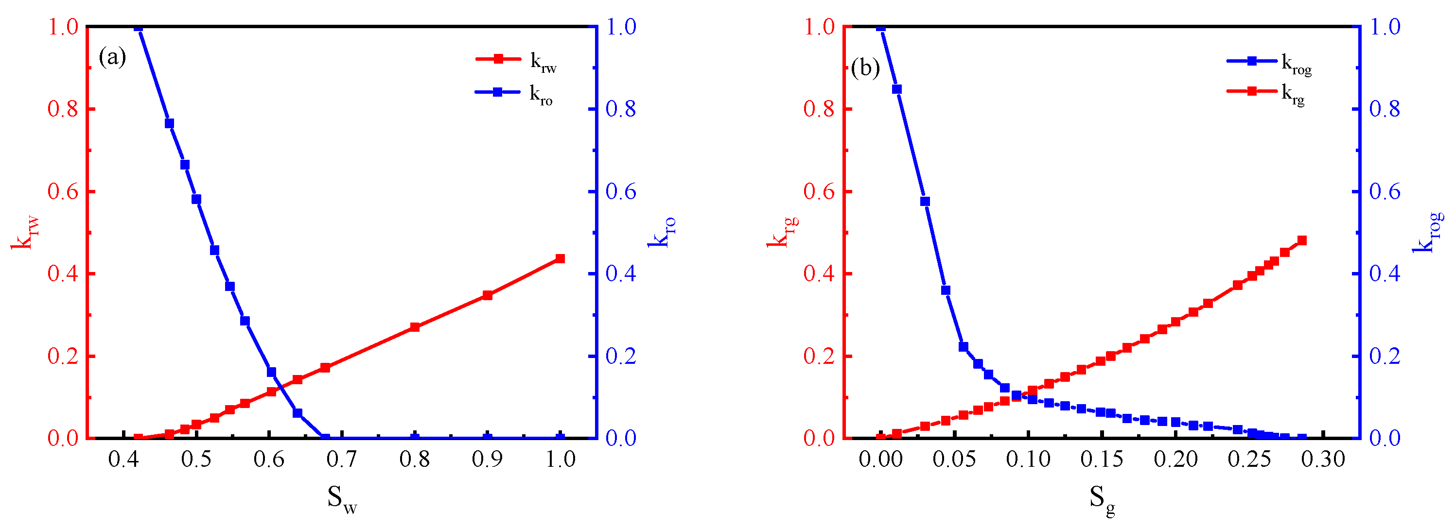
2.3.3. Testing the Relative Permeability Curves Based on Unsteady-State Method
- Oil–water relative permeability curve
- 2.
- Gas–oil relative permeability curve
3. Numerical Simulation
3.1. Simulation for Slim Tube Experiments and 1-D CO2 Flooding
3.1.1. Simulation for Slim Tube Experiments
3.1.2. Simulation for 1-D CO2 Flooding
3.2. Simulation for 2-D CO2 Flooding with Quarter Five-Spot Well Pattern
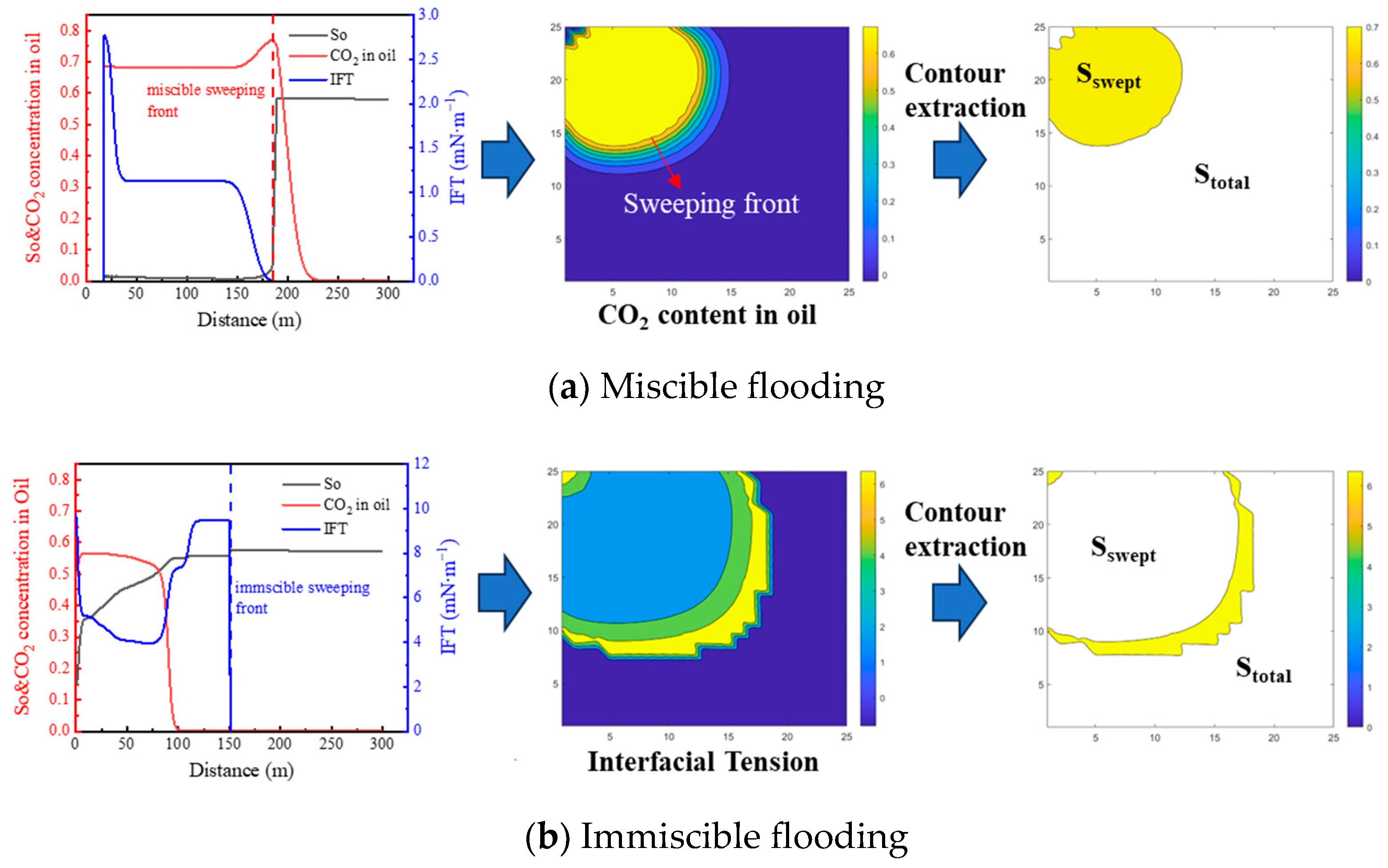
3.3. Solution of Sweep Coefficient for CO2 Flooding
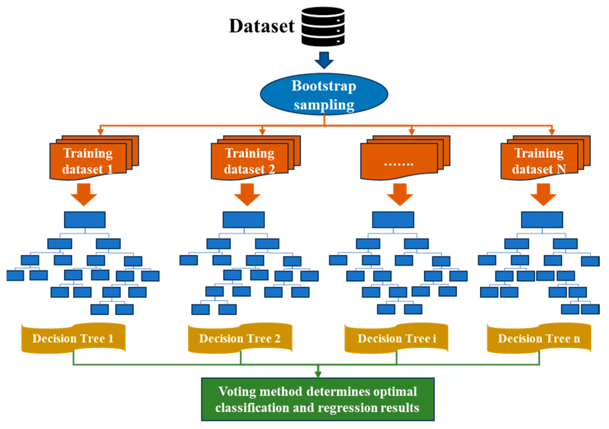
3.4. Main Controlling Factor Assessment of CO2 Flooding Based on Random Forest Algorithm
4. Discussion
4.1. PVT Fitting and Establishment of EOS Equation for Reservoir Fluid
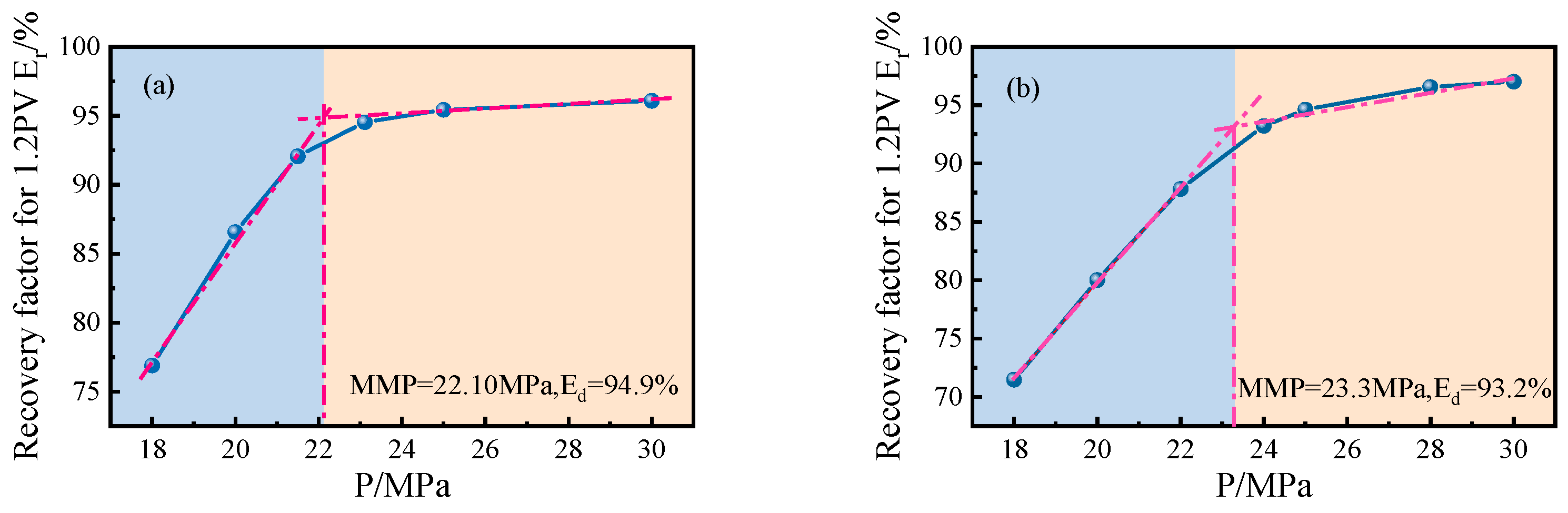
4.2. Determination of Minimum Miscible Pressure Based on Slim Tube Experiment Simulation
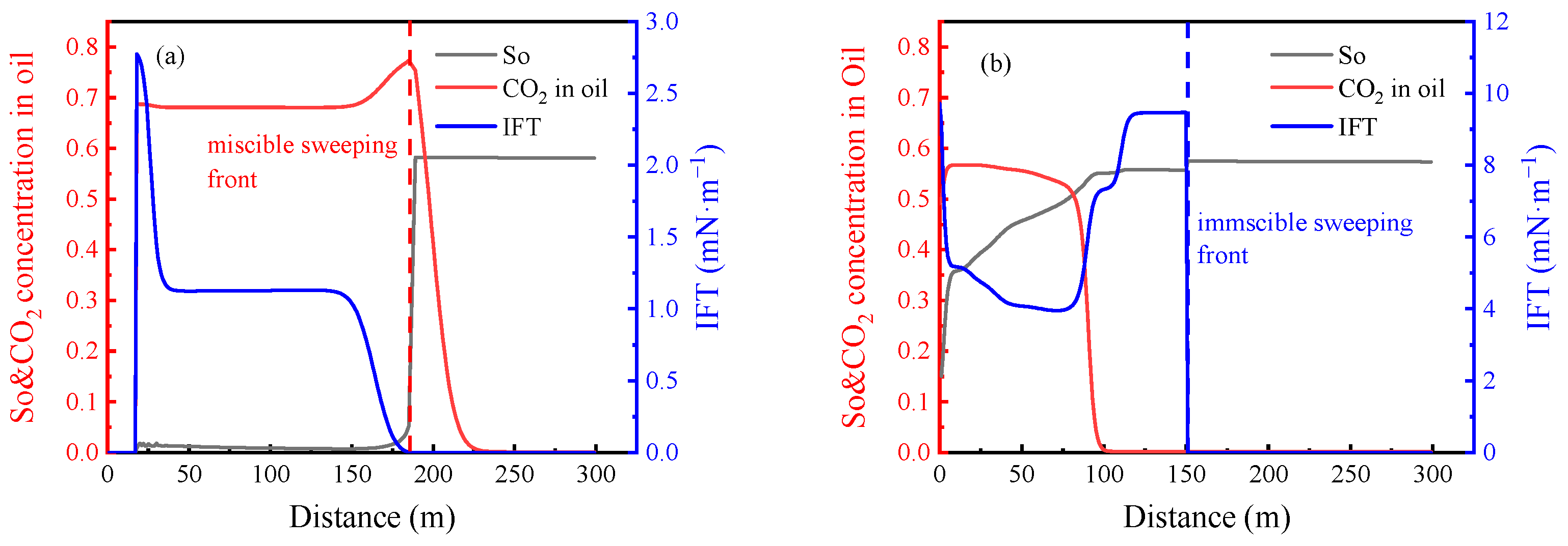
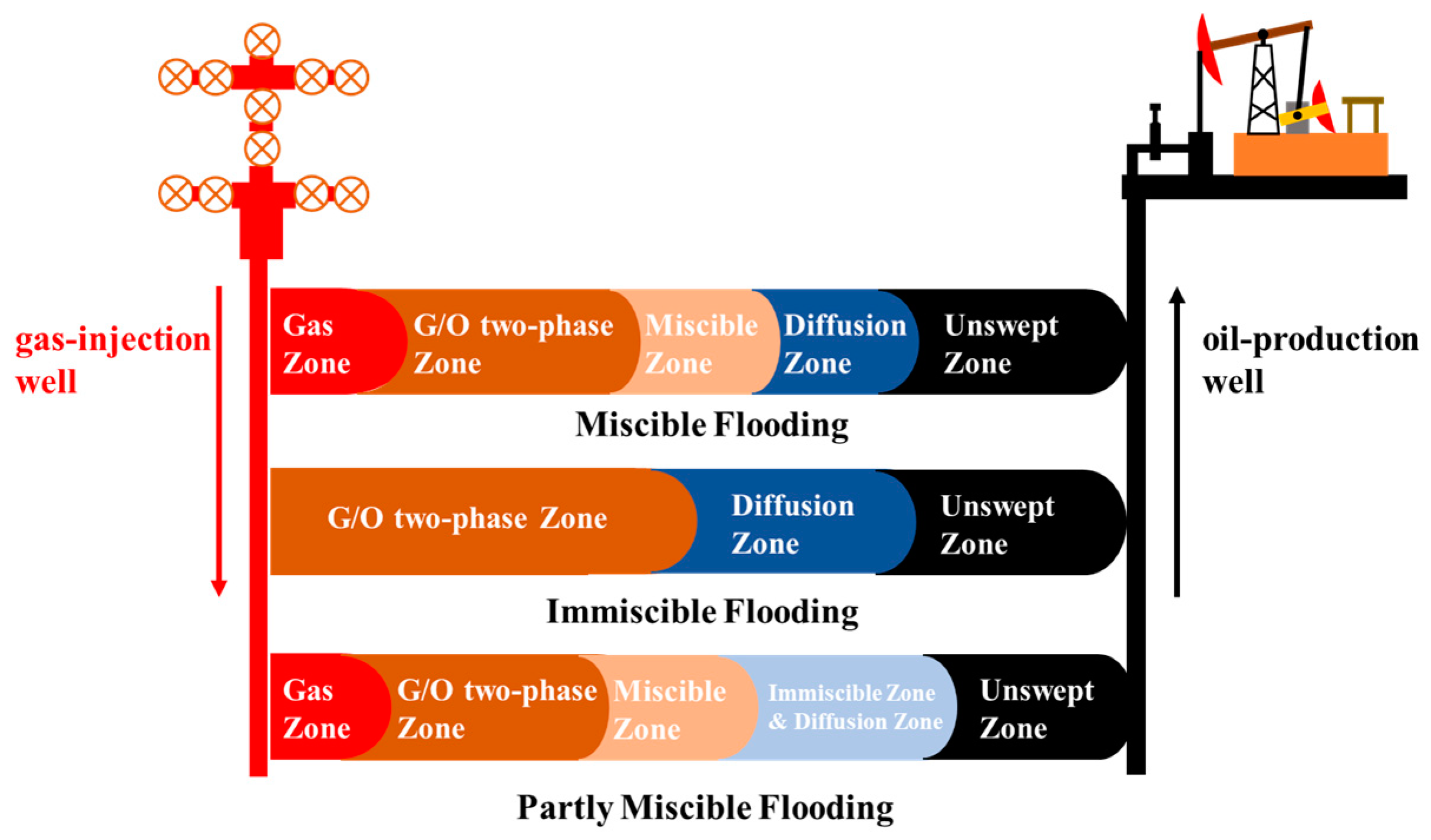
4.3. Front Movement Rules of CO2 Flooding under Different Flooding Patterns
4.4. Front Movement Rules of CO2 Flooding under Different Flooding Patterns
4.4.1. Geological Parameters
- Permeability
- 2.
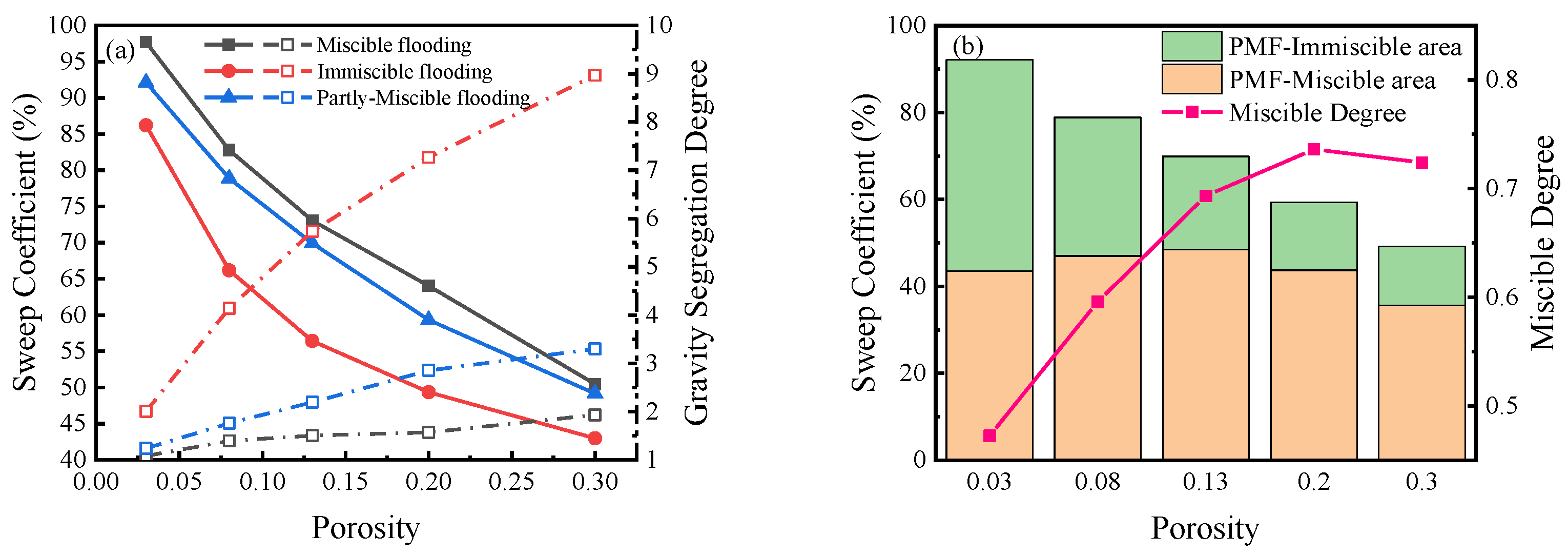
- Porosity
- 3.
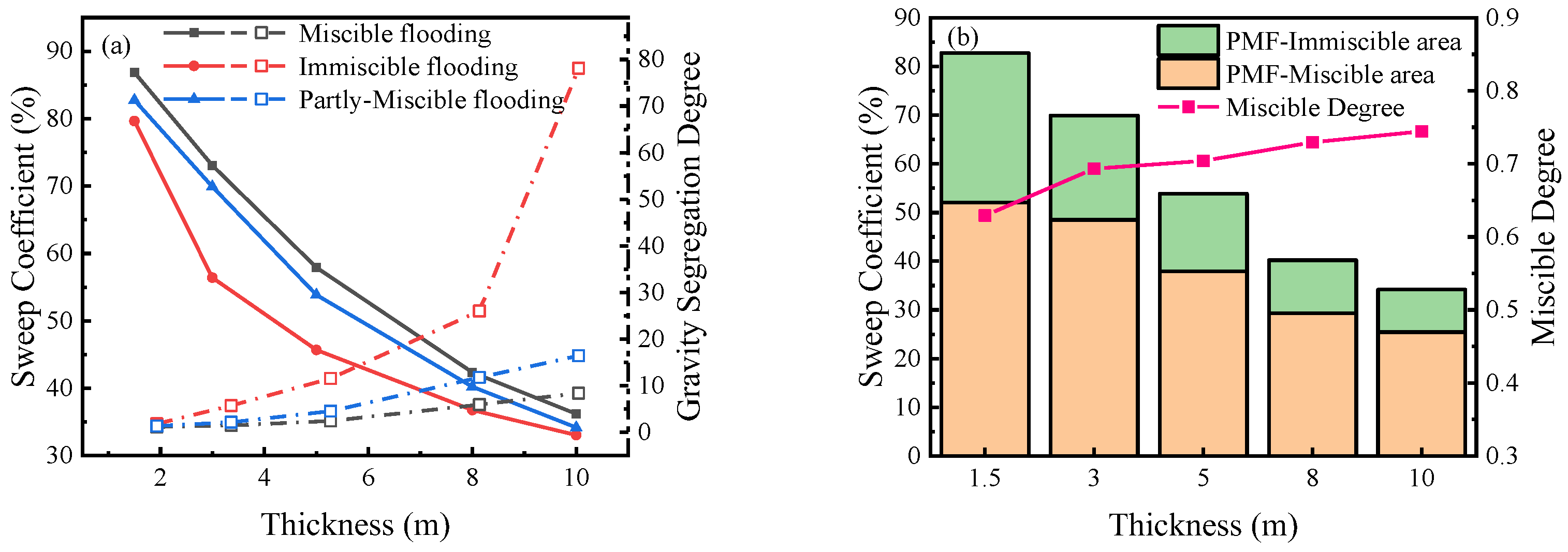
- Reservoir thickness
- 4.
- Permeability Ratio
4.4.2. Injection–Production Parameters
- Well spacing
- 2.
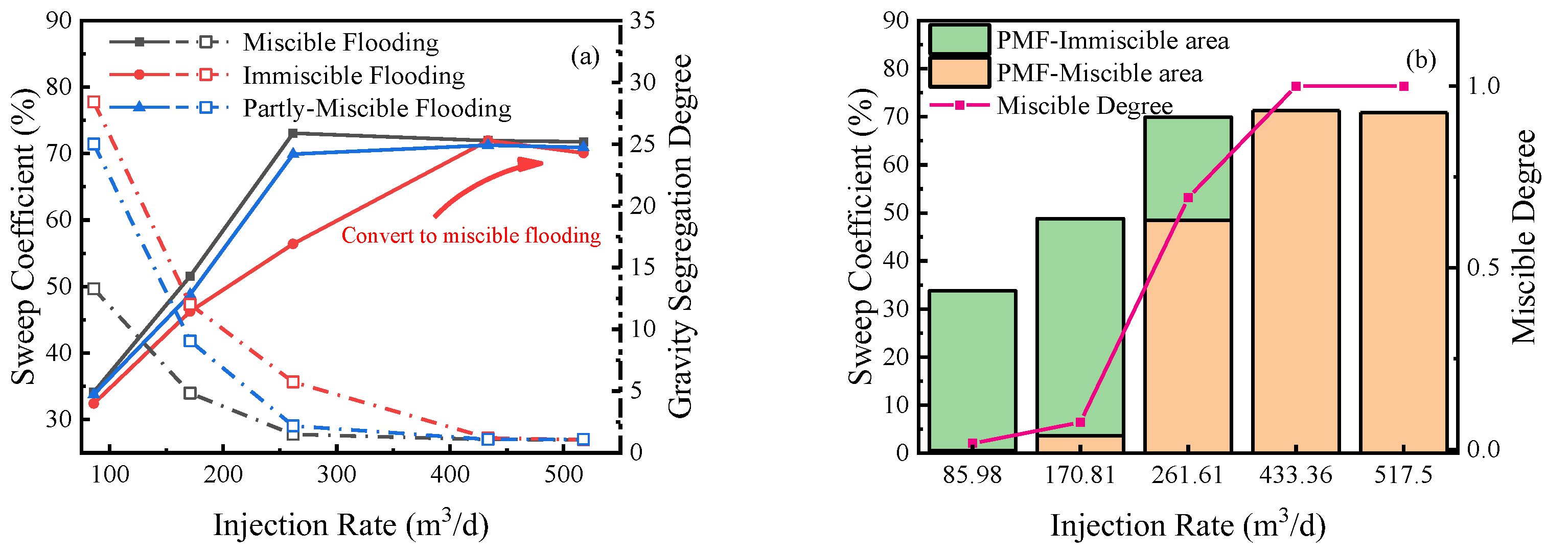
- Gas injection rate
4.4.3. Crude Oil Viscosity
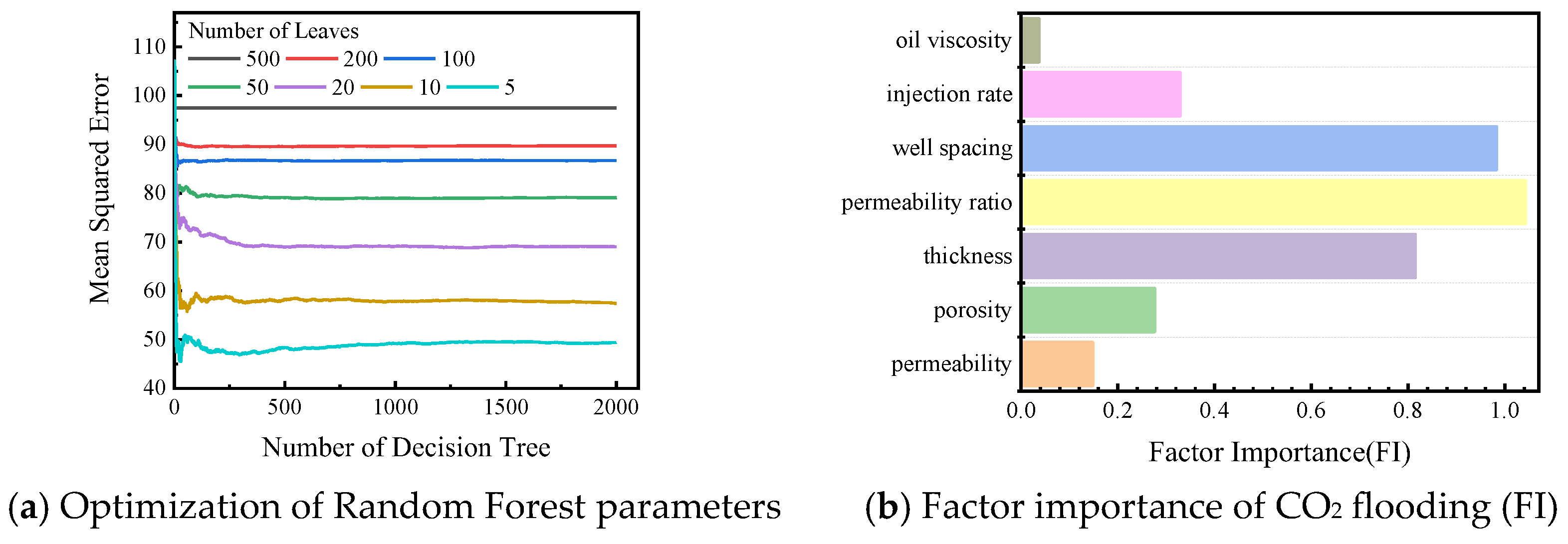
4.5. Analysis of the Main Controlling Factors of CO2 Flooding Sweep Coefficient Based on the Random Forest Algorithm
5. Conclusions
Author Contributions
Funding
Data Availability Statement
Acknowledgments
Conflicts of Interest
References
- McLaughlin, H.; Littlefield, A.A.; Menefee, M.; Kinzer, A.; Hull, T.; Sovacool, B.K.; Bazilian, M.D.; Kim, J.; Griffiths, S. Carbon capture utilization and storage in review: Sociotechnical implications for a carbon reliant world. Renew. Sustain. Energy Rev. 2023, 177, 113215. [Google Scholar] [CrossRef]
- Kumar, N.; Augusto Sampaio, M.; Ojha, K.; Hoteit, H.; Mandal, A. Fundamental aspects, mechanisms and emerging possibilities of CO2 miscible flooding in enhanced oil recovery: A review. Fuel 2022, 330, 125633. [Google Scholar] [CrossRef]
- Zhao, C.; Ju, S.; Xue, Y.; Ren, T.; Ji, Y.; Chen, X. China’s energy transitions for carbon neutrality: Challenges and opportunities. Carbon Neutrality 2022, 1, 7. [Google Scholar] [CrossRef]
- Zhao, K.; Jia, C.; Li, Z.; Du, X.; Wang, Y.; Li, J.; Yao, Z.; Yao, J. Recent Advances and Future Perspectives in Carbon Capture, Transportation, Utilization, and Storage (CCTUS) Technologies: A Comprehensive Review. Fuel 2023, 351, 128913. [Google Scholar] [CrossRef]
- Yuan, S.; Ma, D.; Li, J.; Zhou, T.; Ji, Z.; Han, H. Progress and prospects of carbon dioxide capture, EOR-utilization and storage industrialization. Pet. Explor. Dev. 2022, 49, 955–962. [Google Scholar] [CrossRef]
- Yue, P.; Zhang, R.; Sheng, J.J.; Yu, G.; Liu, F. Study on the Influential Factors of CO2 Storage in Low Permeability Reservoir. Energies 2022, 15, 344. [Google Scholar] [CrossRef]
- Tsopela, A.; Bere, A.; Dutko, M.; Kato, J.; Niranjan, S.C.; Jennette, B.G.; Hsu, S.Y.; Dasari, G.R. CO2 injection and storage in porous rocks: Coupled geomechanical yielding below failure threshold and permeability evolution. Pet. Geosci. 2022, 28, 1. [Google Scholar] [CrossRef]
- Haeri, F.; Myshakin, E.M.; Sanguinito, S.; Moore, J.; Crandall, D.; Gorecki, C.D.; Goodman, A.L. Simulated CO2 storage efficiency factors for saline formations of various lithologies and depositional environments using new experimental relative permeability data. Int. J. Greenh. Gas Control 2022, 119, 103720. [Google Scholar] [CrossRef]
- Wei, J.; Zhou, X.; Zhou, J.; Li, J.; Wang, A. Experimental and simulation investigations of carbon storage associated with CO2 EOR in low-permeability reservoir. Int. J. Greenh. Gas Control 2021, 104, 103203. [Google Scholar] [CrossRef]
- Li, L.; Su, Y.; Sheng, J.J.; Hao, Y.; Wang, W.; Lv, Y.; Zhao, Q.; Wang, H. Experimental and Numerical Study on CO2 Sweep Volume during CO2 Huff-n-Puff EOR Process in Shale Oil Reservoirs. Energy Fuels 2019, 33, 4017–4032. [Google Scholar] [CrossRef]
- Wang, X.; Gu, Y. Oil Recovery and Permeability Reduction of a Tight Sandstone Reservoir in Immiscible and Miscible CO2 Flooding Processes. Ind. Eng. Chem. Res. 2011, 50, 2388–2399. [Google Scholar] [CrossRef]
- Bikkina, P.; Wan, J.; Kim, Y.; Kneafsey, T.J.; Tokunaga, T.K. Influence of wettability and permeability heterogeneity on miscible CO2 flooding efficiency. Fuel 2016, 166, 219–226. [Google Scholar] [CrossRef]
- Zargar, G.; Bagheripour, P.; Asoodeh, M.; Gholami, A. Oil-CO2 minimum miscible pressure (MMP) determination using a stimulated smart approach. Can. J. Chem. Eng. 2015, 93, 1730–1735. [Google Scholar] [CrossRef]
- Han, L.; Gu, Y. Optimization of Miscible CO2 Water-Alternating-Gas Injection in the Bakken Formation. Energy Fuels 2014, 28, 6811–6819. [Google Scholar] [CrossRef]
- Li, L.; Zhou, X.; Su, Y.; Xiao, P.; Chen, Z.; Zheng, J. Influence of Heterogeneity and Fracture Conductivity on Supercritical CO2 Miscible Flooding Enhancing Oil Recovery and Gas Channeling in Tight Oil Reservoirs. Energy Fuels 2022, 104, 103203. [Google Scholar] [CrossRef]
- Guo, Y.; Liu, F.; Qiu, J.; Xu, Z.; Bao, B. Microscopic transport and phase behaviors of CO2 injection in heterogeneous formations using microfluidics. Energy 2022, 256, 124524. [Google Scholar] [CrossRef]
- Alhosani, A.; Lin, Q.; Scanziani, A.; Andrews, E.; Blunt, M.J. Pore-scale characterization of carbon dioxide storage at immiscible and near-miscible conditions in altered-wettability reservoir rocks. Int. J. Greenh. Gas Control 2021, 105, 103232. [Google Scholar] [CrossRef]
- Seyyedi, M.; Sohrabi, M. Assessing the Feasibility of Improving the Performance of CO2 and CO2-WAG Injection Scenarios by CWI. Ind. Eng. Chem. Res. 2018, 57, 11617–11624. [Google Scholar] [CrossRef]
- Liu, Y.; Rui, Z. A Storage-Driven CO2 EOR for a Net-Zero Emission Target. Engineering 2022, 18, 79–87. [Google Scholar] [CrossRef]
- Al-Bayati, D.; Saeedi, A.; Myers, M.; White, C.; Xie, Q.; Clennell, B. Insight investigation of miscible SCCO2 Water Alternating Gas (WAG) injection performance in heterogeneous sandstone reservoirs. J. CO2 Util. 2018, 28, 255–263. [Google Scholar] [CrossRef]
- Ren, B.; Littlefield, J.; Jia, C.; Duncan, I. Impact of Pressure-Dependent Interfacial Tension and Contact Angle on Capillary Trapping and Storage of CO2 in Saline Aquifers. In Proceedings of the SPE Annual Technical Conference and Exhibition, San Antonio, TX, USA, 2–7 October 2023. [Google Scholar]
- Song, X.; Wang, F.; Ma, D.; Gao, M.; Zhang, Y. Progress and prospect of carbon dioxide capture, utilization and storage in CNPC oilfields. Pet. Explor. Dev. 2023, 50, 229–244. [Google Scholar] [CrossRef]
- Kalteyer, J. A Case Study of SACROC CO2 Flooding in Marginal Pay Regions: Improving Asset Performance. In Proceedings of the SPE Improved Oil Recovery Conference, Virtual, 31 August–4 September 2020. [Google Scholar]
- Zhao, X.; Liao, X. Evaluation Method of CO2 Sequestration and Enhanced Oil Recovery in an Oil Reservoir, as Applied to the Changqing Oilfields, China. Energy Fuels 2012, 26, 5350–5354. [Google Scholar] [CrossRef]
- Chen, X.; Li, Y.; Tang, X.; Qi, H.; Sun, X.; Luo, J. Effect of gravity segregation on CO2 flooding under various pressure conditions: Application to CO2 sequestration and oil production. Energy 2021, 226, 120294. [Google Scholar] [CrossRef]
- Al Hinai, N.M.; Saeedi, A.; Wood, C.D.; Myers, M.; Valdez, R.; Sooud, A.K.; Sari, A. Experimental Evaluations of Polymeric Solubility and Thickeners for Supercritical CO2 at High Temperatures for Enhanced Oil Recovery. Energy Fuels 2018, 32, 1600–1611. [Google Scholar] [CrossRef]
- Sun, X.; Long, Y.; Bai, B.; Wei, M.; Suresh, S. Evaluation and Plugging Performance of Carbon Dioxide-Resistant Particle Gels for Conformance Control. SPE J. 2020, 25, 1745–1760. [Google Scholar] [CrossRef]
- Li, Z.; Su, Y.; Li, L.; Hao, Y.; Wang, W.; Meng, Y.; Zhao, A. Evaluation of CO2 storage of water alternating gas flooding using experimental and numerical simulation methods. Fuel 2022, 311, 122489. [Google Scholar] [CrossRef]
- Alsumaiti, A.M.; Hashmet, M.R.; Alameri, W.S.; Antodarkwah, E. Laboratory Study of CO2 Foam Flooding in High Temperature, High Salinity Carbonate Reservoirs Using Co-injection Technique. Energy Fuels 2018, 32, 1416–1422. [Google Scholar] [CrossRef]
- Song, Y.; Yang, W.; Wang, D.; Yang, M.; Jiang, L.; Liu, Y.; Zhao, Y.; Dou, B.; Wang, Z. Magnetic resonance imaging analysis on the in-situ mixing zone of CO2 miscible displacement flows in porous media. J. Appl. Phys. 2014, 115, 401–410. [Google Scholar] [CrossRef]
- Wang, H.; Tian, L.; Chai, X.; Wang, J.; Zhang, K. Effect of pore structure on recovery of CO2 miscible flooding efficiency in low permeability reservoirs. J. Pet. Sci. Eng. 2021, 208, 109305. [Google Scholar] [CrossRef]
- Chen, M.; Cheng, L.; Cao, R.; Lyu, C.; Rao, X. Carbon dioxide transport in radial miscible flooding in consideration of rate-controlled adsorption. Arab. J. Geosci. 2020, 13, 1–11. [Google Scholar] [CrossRef]
- Coats, K.H.; Smith, B.D. Dead-End Pore Volume and Dispersion in Porous Media. Soc. Pet. Eng. J. 1964, 4, 73–84. [Google Scholar] [CrossRef]
- Brattekås, B.; Haugen, M. Explicit tracking of CO2-flow at the core scale using micro-Positron Emission Tomography (μPET). J. Nat. Gas Sci. Eng. 2020, 77, 103268. [Google Scholar] [CrossRef]
- Wang, S.; Jiang, L.; Cheng, Z.; Liu, Y.; Song, Y. Experimental study on the CO2-decane displacement front behavior in high permeability sand evaluated by magnetic resonance imaging. Energy 2021, 217, 119433. [Google Scholar] [CrossRef]
- Duraid, A.B.; Ali, S.; Quan, X.; Myers, M.B.; Cameron, W. Influence of Permeability Heterogeneity on Miscible CO2 Flooding Efficiency in Sandstone Reservoirs: An Experimental Investigation. Transp. Porous Media 2018, 125, 341–356. [Google Scholar] [CrossRef]
- Lewis, E.; Dao, E.; Mohanty, K.K. Sweep Efficiency of Miscible Floods in a High-Pressure Quarter Five-Spot Model. SPE J. 2006, 13, 432–439. [Google Scholar] [CrossRef]
- Hao, Y.; Li, J.; Kong, C.; Guo, Y.; Lv, G.; Chen, Z.; Wei, X. Migration behavior of CO2-crude oil miscible zone. Pet. Sci. Technol. 2021, 39, 959–971. [Google Scholar] [CrossRef]
- Li, J.; Cui, C.; Wu, Z.; Wang, Z.; Wang, Z.; Yang, H. Study on the migration law of CO2 miscible flooding front and the quantitative identification and characterization of gas channeling. J. Pet. Sci. Eng. 2022, 218, 110970. [Google Scholar] [CrossRef]
- Li, N.; Tian, J.; Ren, Z. The research on spread rule of CO2 miscible region in low permeability reservoir. Well Test. 2014, 23, 2023101670. [Google Scholar] [CrossRef]
- Al-Abri, A.; Sidiq, H.; Amin, R. Mobility ratio, relative permeability and sweep efficiency of supercritical CO2 and methane injection to enhance natural gas and condensate recovery: Coreflooding experimentation. J. Nat. Gas Sci. Eng. 2012, 9, 166–171. [Google Scholar] [CrossRef]
- Perrin, J.C.; Benson, S. An Experimental Study on the Influence of Sub-Core Scale Heterogeneities on CO2 Distribution in Reservoir Rocks. Transp. Porous Media 2010, 82, 93–109. [Google Scholar] [CrossRef]
- Lu, Y.; Liu, R.; Wang, K.; Tang, Y.; Cao, Y. A study on the fuzzy evaluation system of carbon dioxide flooding technology. Energy Sci. Eng. 2021, 9, 239–255. [Google Scholar] [CrossRef]
- Bai, S.; Song, K.P.; Yang, E.L. Optimization of water alternating gas injection parameters of CO2 flooding based on orthogonal experimental design. Spec. Oil Gas Reserv. 2011, 20, 48–52. [Google Scholar] [CrossRef]
- Chenglong, L. Gas Channeling Influencing Factors and Patterns of CO2-flooding in Ultra-Low Permeability Oil Reservoir. Spec. Oil Gas Reserv. 2018, 25, 82–86. [Google Scholar] [CrossRef]
- Cui, C.; Yan, D.; Yao, T.; Wang, J.; Zhang, C.; Wu, Z. Prediction method of migration law and gas channeling time of CO2 flooding front: A case study of Gao 89-1 Block in Shengli Oilfield. Reserv. Eval. Dev. 2022, 12, 741–747+763. [Google Scholar] [CrossRef]
- Sinha, U.; Dindoruk, B.; Soliman, M.Y. Prediction of CO2 Minimum Miscibility Pressure MMP Using Machine Learning Techniques. In Proceedings of the SPE-Improved Oil Recovery Conference, Virtual, 31 August–4 September 2020. [Google Scholar]


| Comp. | mol. (%) | Comp. | mol. (%) | Comp. | mol. (%) | Comp. | mol. (%) |
|---|---|---|---|---|---|---|---|
| sCO2 | 0.153 | C7 | 3.835 | C17 | 2.249 | C27 | 1.062 |
| N2 | 2.818 | C8 | 5.131 | C18 | 1.999 | C28 | 1.024 |
| C1 | 16.193 | C9 | 4.225 | C19 | 1.921 | C29 | 0.936 |
| C2 | 3.938 | C10 | 3.897 | C20 | 1.764 | C30 | 0.905 |
| C3 | 3.224 | C11 | 3.36 | C21 | 1.604 | C31 | 0.7 |
| IC4 | 1.675 | C12 | 3.256 | C22 | 1.554 | C32 | 0.716 |
| NC4 | 2.978 | C13 | 3.271 | C23 | 1.431 | C33 | 0.548 |
| IC5 | 0.904 | C14 | 2.697 | C24 | 1.385 | C34 | 0.532 |
| NC5 | 2.594 | C15 | 2.746 | C25 | 1.232 | C35 | 0.476 |
| C6 | 2.431 | C16 | 2.208 | C26 | 1.153 | C36+ | 5.275 |
| Parameters | Values |
|---|---|
| Number of grids | 50 × 1 × 1 |
| Grid size | 32 cm × 5.8 mm × 5.8 mm |
| Porosity/% | 0.33 |
| Permeability/mD | 3.2 |
| Injection pressure constraints/MPa | 35.0 |
| Gas injection rate/(PV/d) | 0.1 |
| Parameters | Values |
|---|---|
| Number of grids | 300 × 1 × 1 |
| Grid size | 1 m × 1 m × 1 m |
| Porosity/% | 0.13 |
| Temperature/°C | 97.3 |
| Permeability/mD | 4.5 |
| Initial formation pressure/MPa | 16.0 (immiscible flooding) |
| 22.0 (partly miscible flooding) | |
| 26.0 (miscible flooding) | |
| Gas injection rate/(m3/d) | 0.00195 (reservoir condition) |
| Well bottom pressure constraint/Mpa | 40.0 (upper limit) |
| 10.0 (lower limit) |
| Parameters | Values |
|---|---|
| Number of grids | 25 × 25 × 5 |
| Grid size | 8 m × 8 m × 0.6 m |
| Porosity/% | 0.13 |
| Temperature/℃ | 97.3 |
| Permeability/mD | 4.5 |
| Initial formation pressure/Mpa | 16.0 (immiscible flooding) |
| 22.0 (partly miscible flooding) | |
| 26.0 (miscible flooding) | |
| Gas injection rate/(m3/d) | 0.77 (reservoir condition) |
| Well bottom pressure constraint/Mpa | 40.0 (upper limit) |
| 10.0 (lower limit) |
| Parameters | Minimum Value | Maximum Value | Unit |
|---|---|---|---|
| Permeability | 0.5 | 100 | mD |
| Porosity | 0.05 | 0.2 | / |
| Reservoir thickness | 3.0 | 30.0 | m |
| Permeability ratio | 1.1 | 100 | / |
| Well spacing | 50 | 300 | M |
| Injection rate | 0.1 | 2.0 | m2/d (RC) |
| Oil viscosity | 0.74 | 33.52 | mPa·s |
| Components | mol. (%) | Pc (atm) | Tc (K) | Mw (g/mol) | Vc (m3/kmol) |
|---|---|---|---|---|---|
| CO2 | 0.153 | 72.80 | 304.20 | 44.01 | 0.0940 |
| N2 | 2.818 | 33.50 | 126.20 | 27.99 | 0.0898 |
| C1 | 16.193 | 45.40 | 190.60 | 16.05 | 0.0990 |
| C2 | 3.938 | 48.20 | 305.40 | 30.09 | 0.1480 |
| C3+C4 | 7.877 | 39.02 | 406.11 | 52.38 | 0.2371 |
| C5+C6 | 5.929 | 31.51 | 486.50 | 76.99 | 0.3335 |
| C7-C16 | 31.58 | 19.82 | 624.24 | 148.05 | 0.5701 |
| C17-C26 | 15.87 | 13.63 | 653.87 | 289.86 | 1.2768 |
| C27-C39 | 9.478 | 11.76 | 878.05 | 444.69 | 1.8926 |
| C40+ | 6.164 | 10.60 | 989.31 | 716.21 | 3.2964 |
Disclaimer/Publisher’s Note: The statements, opinions and data contained in all publications are solely those of the individual author(s) and contributor(s) and not of MDPI and/or the editor(s). MDPI and/or the editor(s) disclaim responsibility for any injury to people or property resulting from any ideas, methods, instructions or products referred to in the content. |
© 2023 by the authors. Licensee MDPI, Basel, Switzerland. This article is an open access article distributed under the terms and conditions of the Creative Commons Attribution (CC BY) license (https://creativecommons.org/licenses/by/4.0/).
Share and Cite
Qi, X.; Zhou, T.; Lyu, W.; He, D.; Sun, Y.; Du, M.; Wang, M.; Li, Z. Front Movement and Sweeping Rules of CO2 Flooding under Different Oil Displacement Patterns. Energies 2024, 17, 15. https://doi.org/10.3390/en17010015
Qi X, Zhou T, Lyu W, He D, Sun Y, Du M, Wang M, Li Z. Front Movement and Sweeping Rules of CO2 Flooding under Different Oil Displacement Patterns. Energies. 2024; 17(1):15. https://doi.org/10.3390/en17010015
Chicago/Turabian StyleQi, Xiang, Tiyao Zhou, Weifeng Lyu, Dongbo He, Yingying Sun, Meng Du, Mingyuan Wang, and Zheng Li. 2024. "Front Movement and Sweeping Rules of CO2 Flooding under Different Oil Displacement Patterns" Energies 17, no. 1: 15. https://doi.org/10.3390/en17010015
APA StyleQi, X., Zhou, T., Lyu, W., He, D., Sun, Y., Du, M., Wang, M., & Li, Z. (2024). Front Movement and Sweeping Rules of CO2 Flooding under Different Oil Displacement Patterns. Energies, 17(1), 15. https://doi.org/10.3390/en17010015