The Colourimetric Method for Mixing Time Measurement in Single-Use and Multi-Use Bioreactors—Methodology Overview and Practical Recommendations

Abstract

Mixing time is an important parameter for quantifying the mixing efficiency of a bioreactor system, essential for successful bioprocess development in various branches of the bioengineering sector (e.g., biopharma, biorefineries, food industry and bioreactor design). The colourimetric method is one of the ways of obtaining valuable quantitative data about the mixing process and the liquid flow inside a vessel. This review consists of a catalogue and a discussion of previously published data in which the colourimetric method has been utilised; a critical comparison between the colourimetric and other mixing time measurement methods; an explanation of practical considerations regarding the bioreactor setup and the choice of reagents; a practical guide for requirements for the acquisition of high-quality images of the mixing process; a thorough discussion of aspects connected to the computer image processing of the video material. This review is intended to thoroughly present the versatility of the colourimetric method for mixing time measurement in miscellaneous bioreactor systems, i.e., in classical tanks and modern single-use (disposable) plastic film-based bag-like containers, and to facilitate the implementation of the colourimetric method in new research setups by providing complete and valuable recommendations about each step of the methodology.

1. Introduction

Mixing time is defined as the duration needed to achieve a set level of homogeneity in a mixture from the moment of a tracer addition into a system [1]. The mixing time characteristics can be obtained on a local and global level. The global mixing time corresponds to the homogenisation of liquid in the whole vessel, while the local mixing time is obtained when the overall volume is divided into smaller parts. The mixing characteristic is an important factor in bioprocesses, as it is one of the ways of defining the cell growth environment and its ability to sustain the proper growth of the culture [2]. Mixing time optimisation is the key aspect of chemical and biochemical process development in various areas of modern industry, e.g., biopharma, biorefineries, food industry, or bioreactor design. Mixing time can provide quantitative information on the locations of inhomogeneities, where the biomass can experience insufficient access to nutrients, locally elevated concentrations of extracellularly secreted toxic metabolites and gradients of essential process parameters [3].

There are technique methods for mixing time measurement, which in general can be divided into local methods, where the information on the mixing process is gathered at only one point inside the vessel, and global methods, where the obtained mixing characteristic is based on the observation of the entire volume of liquid present in the multi-use tank of a classical reactor or disposable plastic film-based bag-like container of a single-use bioreactor (SUB) [4,5].

Some examples of mixing time measurement methods are [4,6,7] the temperature method, where a liquid of a different temperature is added to the bulk volume; the conductivity method, with a tracer being an electrolyte solution; planar laser-induced fluorescence (PLIF), in which a fluorescent indicator is being excited by a sheet of laser light; the colourimetric method, where a tracer (i.e., an indicator or a dye) is injected into the liquid and the mixing progress is evaluated based on the colour change of the bulk liquid due to a reaction or change in the concentration of the indicator.

Application of the colourimetric method offers the possibility of non-invasive, detailed observation of liquid flow patterns inside a bioreactor vessel with inexpensive tools and accessible non-toxic chemicals [7]. It is, however, limited by the requirement of optical access into the inside of the examined vessel and by the possibility of parts of the liquid obscuring each other due to the 2D projection of the 3D bioreactor volume [8].

This review paper is set up with two primary goals. The first is to summarise studies in which the colourimetric method was utilised during the experiments. The studies have been grouped according to the type of reactor or bioreactor being characterised. The second goal of this review is to present and explain the steps and requirements that ought to be fulfilled for deploying the colourimetric method at any research facility and, possibly, in new experimental setups. These recommendations are based on the practices implemented previously by different research groups. To our knowledge, this review is the first paper in which the colourimetric method has been covered in-depth with regard to various types of reactors and bioreactors, including providing recommendations for an image analysis and processing, including the newest methods and tools.

Previously published works about mixing time measurement in reactors focus on covering and comparing many methods differing in their fundamental principles, such as the specialised methods covered by Ascanio (2015) [4] or more common methods for determining mixing time and other engineering parameters covered by Löffelholz (2013) [9]. The recommendations for single-use bioreactor characterisation by Bauer et al. [10] include the decolourisation method for mixing time measurement with iodometry but suggest only visual observation and mixing time determination. The paper by Cabaret et al. (2007) [10], while thoroughly covering the topic of colour-changing chemicals and introducing the methods for an image analysis based on colour channel values, does not include statements about colourimetric method application devices other than stirred reactors and does not delve into the technical considerations for image acquisition.

This review is divided into sections dedicated to explaining four main topics crucial in the practical challenges of colourimetric method application for mixing time measurement in various types of bioreactors:

• Section 2. Applications of the Colourimetric Method for Reactor and Bioreactor Studies contains a catalogue of existing papers, which contains results based on the application of the colourimetric method, a discussion about the types of devices in which the colourimetric method has been applied, a comparison of mixing time measurement methods based on experimental data and a discussion about the advantages and shortcomings of visual and computerised image processing.
• Section 3. Laboratory Procedure Considerations contains a listing of colour-changing chemicals that can be used with the colourimetric method, recommendations regarding a typical laboratory procedure for mixing time measurement and a summary of liquids of various rheological characteristics previously analysed in colourimetric method setups.
• Section 4. Image Acquisition contains a discussion about the cases where special adaptation of the camera equipment to the reactor was necessary, with a focus on the acquisition of high-quality image data and a set of recommendations for the camera equipment, image parameters that need to be considered during image acquisition and proper lighting of the experimental setup.
• Section 5. Image Processing contains recommendations for the final step of colourimetric method application, i.e., the suggested order and description of operations during digital image processing, a summary of colour spaces that can be considered in the processing, the definitions of mixing time that have been previously applied in different studies, a discussion about local mixing time and mixing time maps and a summary of software tools that can be used for the application of the colourimetric method.

Information provided in this review paper should facilitate the successful holistic application of the colourimetric method in research facilities, offering an accessible possibility for an in-depth liquid flow analysis in single-use or multi-use bioreactor setups.

2. Applications of the Colourimetric Method for Reactor and Bioreactor Studies

Since the literature mention in the work by Fox and Gex [11], in which mixing time in “cylindrical vessels 1 and 5 ft in diameter” was originally measured through observation of phenolphthalein decolourisation, the colourimetric method has been used extensively during testing and characterisation of vessels and bioreactors of various types and scales. Several variants of the method have been developed, involving different colour-change chemicals, reagents, image processing and analysis techniques and mixing time value definitions. A summary of previously published scientific papers and reports involving the colourimetric method for mixing time measurement, grouped according to the type of system being investigated, is presented in

Table 1. A catalogue of scientific papers and reports in which the colourimetric method has been implemented for mixing time measurement during the experiments.

Working Volume	Commercial Name (If Applicable)	Colour-Changing Reagents	Image Analysis		Notes	Reference
			Software (If Applicable, Version No. If Specified by Authors)	Colour Space (If Applicable)
Stirred tank reactors (multi-use)
22–280 L		phenolphthalein	n/a (visual)			[11]
25–37 L		methyl red	n/a (visual)			[12]
3 L, 13 L		iodine + starch	n/a (visual)			[13]
140 L		iodine + starch	n/a (visual)			[14]
180 L		iodine + starch	n/a (visual)			[15]
7 L		bromothymol blue	n/a (visual)		no quantitative data	[16]
50 L		iodine + starch	n/a (visual)			[17]
30 L		DISMT *	OPTIMAS 6.5	RGB (G channel)		[18]
750 L		bromocresol purple	n/a (visual)			[19]
46 L		bromocresol purple	n/s	RGB (G channel)		[20]
7.8 L, 14.5 L, 200 L		various (see footer) **	n/s (in-house)	RGB (channel depending on indicator)		[10]
30 L		DISMT *	OPTIMAS 6.5	RGB (G channel)		[21]
35 L, 77 L, 190 L		bromocresol purple	n/s (in-house)	RGB (G channel)		[22]
4 L		bromocresol purple	Image-Pro Plus 4.5.1	n/s		[23]
42 L, 340 L		n/s	n/s (in-house)	grayscale		[24]
200 L, 400 L		iodine + starch	n/s	n/s		[25]
10 mL		methylene blue	ImageJ 1.48b6, MATLAB R2012a	grayscale		[26]
5 L		bromocresol purple	n/s	n/s		[27]
15 m3		phenolphthalein	ImageJ	grayscale		[3]
2 L		bromocresol purple	MATLAB	HSV		[28]
12 L		phenolphthalein	ImageJ	RGB		[29]
200 mL	DASGIP® Cellferm-pro	DISMT *	MATLAB	RGB (G channel)	with microcarriers	[30]
3 L		bromothymol blue	n/s	grayscale		[31]
10 L		Cochineal Red	MATLAB R2020a	RGB (R channel)		[32]
3.8 L		bromothymol blue	MATLAB	grayscale	single multi-compartment bioreactor	[2]
250 mL		DISMT *	MATLAB	RGB (G channel)		[33]
Stirred tank reactors (SUBs)
3 L	Mobius CellReady™	iodine + starch	n/s	n/s		[34]
15 mL	Ambr™	iodine + starch	n/a (visual)			[35]
1 L	Allegro™ STR 50	DISMT *	MATLAB	RGB (G channel)	scale-down prototype of a 50 L bioreactor	[36]
Shaken or rocked vessels (shake flasks, orbitally shaken or wave-mixed SUBs)
2 L, 3 L, 30 L, 1500 L	Kühner™ ES-W shaker	DISMT *	n/s (in-house)	RGB (G channel)	orbitally shaken	[37]
100 mL, 250 mL, 500 mL		bromothymol blue	n/a (visual)	n/a	shake flasks	[6]
600 mL	TubeSpin® 600	DISMT *	n/s	RGB (G channel)	orbitally shaken	[38]
2 L, 20 L	BIOSTAT® CultiBag™ RM	iodine + starch	n/a (visual)		shake flasks and rocking bioreactor bags (orbitally shaken or rocked)	[39]
2 L		DISMT *	MATLAB (version n/s)	RGB (G channel)	orbitally shaken	[40,41]
10 L		phenolphthalein	n/a (visual)		rocking (wave-mixed) single-use bioreactor; no quantitative data	[42]
Others
37 L		Purple Drimarene R 2 RL	n/s (in-house)	grayscale	bubble column	[43]
120 mL		bromophenol blue	n/s	RGB	soft elastic reactor	[44]
10 L		Patent Blue V (E131) dye	VLC 3.0.16, IrfanView 4.58, GIMP 2.10.24	grayscale	plastic bag bubble photobioreactor	[45]

* Double Indicator System for Mixing Time—a methyl red and thymol blue indicator system. ** pH indicators used: bromocresol purple, bromothymol blue, cresol red, methyl red, phenolphthalein, phenol red. n/a—not applicable; n/s—not specified.

.

2.1. Applications of the Colourimetric Method across Types of Devices

The biggest number of previously published papers, which included the colourimetric method for determination of mixing time, regarded stirred tank reactors and bioreactors, including, in some cases, single-use bioreactors [34,35,36]. The investigations included baffled and unbaffled classical tanks agitated with various equipment: Rushton turbines [3,10,15,16,17,19,24,25,27,28,31,32,33] and their variants (Scaba SRGT [15]), pitched-blade impellers [3,10,17,24,25,33], disk turbines [19], elephant ear [27,36] and marine blade impellers [27,34,35], hydrofoil [14], Maxblend™ [10,22,23], helical ribbon [13,18,29], a trapezoidal paddle [30], axial flow impellers [24] and planetary [18,21] and coaxial mixers [20]. Some papers contained results from experiments involving orbitally shaken devices, i.e., shake flasks [6], orbitally-shaken single-use bioreactors [37,38,40,41] and wave-mixed single-use bioreactors agitated on an orbitally shaken [39] or a rocking platform [39,42]. A few publications contained results and observations of mixing performance inside other devices, such as a bubble column [43], a soft elastic reactor [44] and a plastic bag photobioreactor [45].

Typically, the maximum volume of the vessel analysed using the colourimetric method was no larger than 1000 L. The volume of analysed vessels ranged from the millilitre scale [6,27,30,33,38,44], including vessels from parallel bioreactor systems [35], through bench-scale and laboratory-scale devices [16,17,18,20,21,22,24,27,28,29,31,32,34,36,37], up to pilot-scale systems in the hundred-litre range [14,15,19,22,24,25]. However, one has to note the examples of large-scale reactors, such as the 1500 L orbitally shaken single-use plastic film-based bag-like container analysed by Tissot et al. [37] or the 15 m³ stirred tank investigated by Rosseburg et al. [3].

The colourimetric method, which enables researchers to calculate mixing time quantitatively, allows for observing compartmentalisation and segregated zones inside the liquid during the mixing process. These observations have been performed in stirred tanks, e.g., as a way of comparing different combinations and operation modes of impellers mounted inside a vessel [19,20,22,27,28], gathering information about the performance of an impeller in a particular setup [22,23,26,29] or characterising the progress of the mixing process inside commercially available systems, including single-use bioreactors [35,36]. Similar observations have also been performed in disposable orbitally shaken vessels, for example, in the work of Rodriguez et al. [41], where detailed images captured during the decolourisation of methyl red and thymol blue were used to correlate the size of vortical cells inside the liquid phase with the dimensionless mixing number Nt_m for an in-depth analysis of the impact of operational parameters on the flow structure of the mixed liquid phase. A phenolphthalein decolourisation-based method was used in work by Jones et al. [42] for qualitative observation of mixing inside a wave-mixed 10 L single-use bag—however, no detailed analysis of the flow induced by the continuous oscillations of the platform has been performed.

The colourimetric method has been extensively used during studies of orbitally shaken disposable cylinders and flasks across different scales. In the work of Tissot et al. [37], the colourimetric method was used as the source of experimental data for the derivation of a scale-up factor in orbitally shaken vessels of four different sizes and as a means of examining and verifying similar mixing regimes between 1500 L and 30 L scales. Tan et al. [6] proposed a correlation between mixing time and the power input in the turbulent flow regime inside shake flasks in the 100–500 mL scale. Rodriguez et al. [40,41] also showed the relationship between Froude number values and the mixing number.

Gaugler et al., in their work [2], used the colourimetric method for characterising a newly developed single multi-compartment bioreactor (SMCB), which allows for the recreation of large-scale mixing behaviour in a small-scale vessel. In the study, special discs with different arrangements of holes were used to divide the tank volume into compartments, allowing for the adjustment of mixing time values to simulate the conditions inside a large-scale tank during scale-down approaches. Data about the mixing process gathered through observations and a further analysis of video material were used to derive empirical correlations for calculating the area of perforations on the discs depending on the desired mixing time value and the power input in the bioreactor.

A notable example of colourimetric method application is presented in the paper of Xiao et al. [44], in which a quantitative comparison of mixing states by calculating spatial and frequency distributions of the mixing level inside a soft-elastic reactor (SER) was presented based on the extensive analysis of images captured during the decolourisation of a bromophenol blue indicator. The recording and subsequent analysis of the video material provided insight into the complicated mixing mechanism of the investigated system.

The above examples show that the colourimetric method is well suited for scale-up, scale-down, performance and characterisation studies of various types of reactor and bioreactor systems, including novel and prototyped devices, the properties of which have not yet been well systematised. The following chapters and subsections of this review contain recommendations structured around different aspects of colourimetric method implementation aimed at shortening and facilitating the steps necessary for successfully applying similar procedures in new experimental setups.

2.2. Comparisons between Mixing Time Measurement Methods

Some papers in the field include comparisons between results obtained using various mixing time measurement methods performed in identical experimental setups. Care should be taken during these comparisons, as the methods inherently differ in the phenomena being observed as indications of the mixing process, the applied definitions of mixing time and the invasiveness and locality of the measurement. The methods most often mentioned next to the colourimetric method are

• the sensor method, based on recording temporal changes in the readings of one or more sensors placed inside the mixed liquid, including

  ○

  the thermal method, in which temperature sensors such as thermocouples monitor the changes in liquid temperature after injection of a small portion of liquid of a different temperature [46];

  ○

  the conductivity and pH methods, which rely on measuring changes in conductivity or pH after introducing a tracer with conductometric or pH electrodes [47].

• planar laser-induced fluorescence (PLIF), in which the mixing is observed through the dispersion of a fluorescent dye excited by a sheet of laser light, resulting in the emission of light at a specific wavelength [48].

Kraume and Zehner [17] applied the iodine–starch decolourisation and conductivity methods to characterise homogenisation efficiency in a baffled tank with a pitched blade or a Rushton turbine. The authors found that the results obtained with both methods were similar, with 10–20% scattering of values across the stirrer speed range. Different accuracies of results are reported depending on the impeller type. In the case of the pitched blade turbine, the scattering was more significant, and the values from the decolourisation method were higher than those from the sensor method.

Trad et al. [27] and Chezeau et al. [28] have directly compared results obtained with colourimetric, conductivity and PLIF methods in small-scale bioreactors agitated with different impellers. The authors of [28] emphasised that for each method, the same volume of tracer was injected in explicitly defined places and that the mixing time was defined as the moment of reaching 95% homogeneity. The authors conclude that the results obtained with the three methods were similar. However, in the case of [28], discrepancies could be observed in the transitional flow regime, where the sensor method values were higher than those obtained with two other methods. Shortcomings of the sensor method are pointed out, namely the dependency on probe placement and the inability to examine flow patterns [27]. The decolourisation and PLIF methods were supplemented with digital image processing, which could improve their accuracy. It is mentioned that the decolourisation method may underestimate mixing time values that are under 10 s and is subject to errors due to the obscuring of the parts of liquid further from the camera by the regions in front of the vessel [28]. However, the authors point out the PLIF’s disadvantage of a high cost, focused mainly in the laser and camera hardware [27].

2.3. Visual Observations and Computerised Image Processing

Among the various approaches to processing captured video data, a significant distinction can be made between visual observations and computerised digital image processing. Before the advent of inexpensive and powerful computers, visual observations or a visual analysis of image frames by the observer performing the measurement were prevalent in studies involving the colourimetric method. A visual image analysis has substantial disadvantages, given the inherent subjectivity of colour perception of the observer [10], which limits the repeatability and reproducibility of results; high labour costs; and limited ability to perform measurements in which low mixing time values characterise the mixing process. In the work of Fox and Gex [11], the authors attempted to limit the errors in visual interpretation through independent simultaneous determination of the measurement endpoint by two observers. The authors point out that in most cases, the results agreed within 10%, but deviations as high as 60% also occurred. Despite these shortcomings, Lamberto et al. [16] still point out the advantages of a visual analysis, mainly compared to the sensor methods, which involve introducing probes into the liquid, which disturb flow patterns meant to be measured.

The work of Delaplace et al. [18] is the first example present in the literature of mixing process images being digitally analysed with the aid of computer software. In that study, the temporal changes in RGB values of frames acquired with a digital webcam at a temporal resolution of 1 Hz were processed with a macro written for commercial OPTIMAS software. Nearly all papers published after the work of Delaplace et al. [18] involved a computer image analysis in some form, with differences in the image acquisition hardware, data processing software and definitions of mixing time used for calculating results. A summary of techniques, software and requirements for a digital image analysis is presented in Section 5.

3. Laboratory Procedure Considerations

The literature regarding the colourimetric method gives a few examples of the reagents and colour-changing chemicals that can be used in laboratory procedures. They can be generally arranged into two main categories:

• Physical methods (without a chemical reaction)—observation of the mixing process is based on the temporal changes in concentration of a dye dissolving in the bulk of the liquid. The dye does not change its chemical structure during mixing. Examples of dyes that have been used in studies with the colourimetric method are methylene blue [26], Cochineal Red [32], Purple Drimarene R 2 RL [43] and Patent Blue V E131 [45].
• Chemical methods (with a chemical reaction)—the progress of the mixing process is assumed using the colour change in a chemical, which changes its properties based on an instantaneous chemical reaction [49]. The frequently used chemical reactions are

  ○

  A redox reaction between iodine/triiodide (i.e., ${\mathrm{I}}_2$/${\mathrm{I}}_3^{-}$ ions) and thiosulfate anions, ${\mathrm{S}}_2{\mathrm{O}}_3^{2-}$, in a starch solution [13], usually called the iodometric reaction. During the reaction, the iodine/triiodide is reduced into an iodide, ${\mathrm{I}}^{-}$, anion, which makes the dissolved starch change from deep purple to colourless. This reaction was applied during studies of multi-use reactors [13,14,15,17,25] and single-use bag-like containers [34,35,39]. The disadvantage of the iodometric reaction with applications in SUB setups is the possible interaction between iodine and the polymer film of the single-use bag, which can lead to staining and gradual deterioration of the optical properties of the disposable container.

  ○

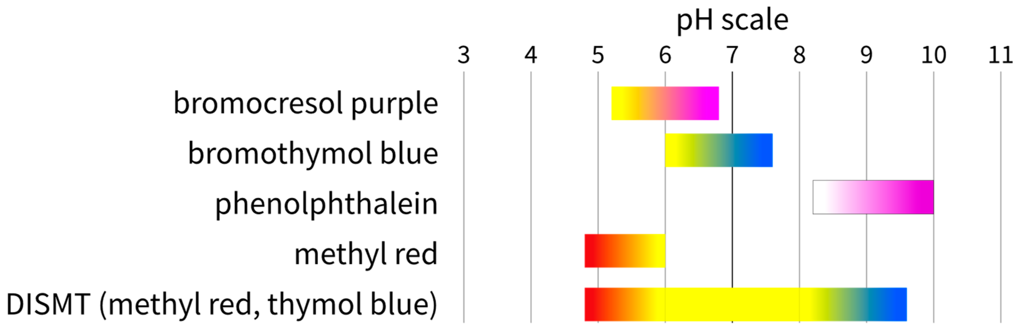
  An acid–base neutralisation reaction in the presence of one or more pH indicators. The chemicals used during the experiments were usually strong bases and acids, like sodium hydroxide and hydrochloric acid, at various concentrations depending on the setup and the indicator pH colour change range. One or more indicators in one solution can be added during the experiments. Examples of the pH indicator systems that have been used with the colourimetric method are listed in

  Table 2. pH indicators used in colourimetric method studies (based on Cabaret et al. [10]).

  Indicator	Colour at Low pH	pH Colour Change Range	Colour at High pH	Reference
  Single indicator systems
  bromocresol purple	yellow	5.2–6.8	purple	[19,20,22,23,27,28]
  bromothymol blue	yellow	6.0–7.6	blue	[2,6,16,31]
  phenolphthalein	colourless	8.2–10.0	pink	[3,11,29,42]
  methyl red	red	4.8–6.0	yellow	[12]
  Double indicator systems
  DISMT (methyl red, thymol blue)	red	4.8–9.6	blue	[18,21,30,33,36,37,38,40,41]

  . The colour ranges of the indicator are summarized in Figure 1.

With the physical methods, in which no chemical reaction occurs, the mixing progress is only determined based on the dilution of the dye. With this, a given portion of liquid can appear mixed within the sampling equipment’s finite resolution but not molecularly mixed. With chemical-reaction-based diagnostics, the reagent molecules must come into contact to allow colour change [50].

The typical laboratory procedure for mixing time determination using the colourimetric method is summarised in Figure 2. The primary step is filling the vessel with a starting solution consisting of the starting reagent at a given concentration with a small amount of the indicator dissolved. A small volume of the tracer solution is rapidly injected into the liquid after the starting solution is brought to the correct agitation and environment conditions. The concentration of the tracer solution should be significantly higher than the starting solution, which will minimise the total volume of the tracer needed to bring the solution to the final colour.

The amount and concentration of the tracer needed for a single injection are related to the molar ratio of the acid and base. The molar ratio can influence the repeatability of measurements and whether micro- or macromixing time is to be measured. At a reagent molar ratio of 1:1, a stoichiometric mixture is obtained. In this case, for the mixing to be complete, every molecule of the tracer has to come into contact with a starting reagent molecule, and the micromixing time can be measured [10,31]. At this ratio, the longest mixing time values, also called “terminal mixing times”, will be obtained. However, since obtaining an exact 1:1 ratio of reagents is difficult in laboratory conditions, the micromixing time measurements with the colourimetric method can be unreliable, with significant deviations in values between individual measurements and poor repeatability [1].

Usually, a higher reagent molar ratio should lead to obtaining more reliable results and improve measurement repeatability. In this case, more than one tracer molecule can come into contact with each molecule of the starting reagent, which means that the mixed appearance of the liquid can be achieved without perfect mixing on the molecular level. Some authors recommend a reagent molar ratio not smaller than 2:1. After this threshold, the reliability is greatly improved, and the results represent the macromixing time in the studied systems [1]. In the case of bioreactors, given the living cells’ metabolism rate, the macromixing time is sufficient for evaluating whether the conditions inside a vessel are suitable for a given bioprocess [31].

It is recommended that the experiments are performed as partial or complete decolourisation, in which the indicator colour in the starting solution is darker and more saturated than in the final, mixed state. When decolourisation is applied, the remaining unmixed darker areas of liquid are easier to distinguish from the lightly coloured bulk of the liquid in a 2D projection of a 3D vessel volume. In an opposite scenario, the darker mixed regions of liquid can obscure and cover the lighter areas, making them less visible, which can cause the measurement endpoint to be more difficult to detect [7,8] and the resulting mixing time values underestimated [46].

Fitschen et al. [31] point out the advantage of colour-changing chemicals, which do not become colourless at the end of the measurement (e.g., phenolphthalein). Applying an indicator exhibiting two distinct, contrasting colours can allow for investigations of the flow pattern and intermediate zones, enabling the researchers to obtain more information about the temporal progress of the mixing process.

The DISMT system, i.e., the Double Indicator System for Mixing Time, was developed by Melton et al. [50]. The methodology relies on the colour change in two independent pH indicators: methyl red and thymol blue. Liquid during the measurement with the DISMT system is red at a pH smaller than 4.8 and blue at a pH bigger than 9.6. Between those values, i.e., in the pH range 4.8–9.6, both indicators are yellow, indicating that the liquids are “mixed within tolerance”. The system allows for capturing compartments inside the liquid in which there is overconcentration of either the base or the acid, improving the ability to detect intermediate zones. However, applying the DISMT scheme requires pH balancing of the solutions used before measurement to ensure the 1:1 ratio of the acidic and alkaline chemicals.

With the colourimetric method, it is possible to analyse mixing in liquids of different rheological properties: non-Newtonian solutions of sodium carboxymethyl cellulose (CMC) [20,22,24,29,43], polyacrylamide [13], xanthan gum [19,22,24] or Newtonian mixtures of water with glucose syrup [10,18,19,20,22,23], glycerin [13], polyalkene glycol [28] and polyethylene glycol [43].

4. Image Acquisition

Image acquisition is a crucial step in the application of the colourimetric method. The quality of frames in the video material will directly influence its usability. Properties of the experimental setup in which the colourimetric method will be used, adaptation of the filming equipment to the setup characteristics, use of sufficient quality filming equipment and proper adjustment of image parameters are the factors that need to be considered in the planning and preparations for the deployment.

4.1. Properties of the Device for Characterisation

An essential part of successfully implementing the colourimetric method in a new experimental setup is considering the device’s properties for characterisation, which will influence the placement and mounting of the camera equipment. The first requirement for applying the colourimetric method is an optical window allowing for observing the contents inside the vessel. In general, it is preferred that the vessel be made entirely from transparent material, which is sometimes fulfilled by the design of the device. An example is the case of single-use bioreactors, where the culture bag is made from multi-layer plastic film [51] or, as in small-scale stirred SUBs [34,35], from rigid plastic material. Sources also report the use of vessels made from glass [2,16,21,24,26,28,31,43,48], acrylic/plexiglass [3,13,15,24,25,33,36,52] or polycarbonate [10,19,53].

In cases where the device to be characterised is made from a non-transparent material, it may be necessary to construct a 3D mimic that reflects the geometry of the original equipment. The requirement of optical access to the insides of the vessel is the limiting factor of the applicability of the colourimetric method in industrial-scale systems [3]. Satisfying this requirement is more challenging, given the cost and feasibility of manufacturing large structural parts with good mechanical and optical properties.

The considerations should also focus on the shape of the device’s vessel and internal equipment, whether it is stationary or performs movement, and the characteristics of the liquid agitation mechanism. In most cases, as in the case of stirred bioreactors, the vessel walls are usually stationary, and the only moving parts of the device are the rotating agitator and its shaft. Therefore, the camera can usually be mounted stationarily in front of the tank with a view of a plane parallel to its vertical axis [2,28,29,32] (Figure 3). In their papers regarding the characterisation of small-scale cylindrical vessels, some authors mention placing the device inside a separate rectangular vessel filled with liquid of a similar composition and refractive index to the one inside the tank [10,20,22,29,30,31,48,53]. This approach is used to minimise the distortions from the curved tank walls.

In some cases, rotation of the agitation equipment and changes in its apparent shape during the rotation cycle can introduce noise and partial obstructions of the view of some parts of the liquid inside the vessel. The effects of these disturbances should be considered during the postprocessing of image data. Iranshahi et al. [23] in their work used a Maxblend™ impeller, which has a large surface area and covers the majority of tank volume during the rotation cycle. During the image processing, the authors selected frames in which the agitator is perpendicular to the camera, corresponding to the moments in which the apparent area of the agitator is minimal. Analogously, Xiao et al. [44], during studies with a soft-elastic reactor, only selected the frames in which the beating slider crank is not pressing on the repetitively deformed walls of the vessel. These approaches can limit the temporal resolution of the measurement or be non-feasible depending on the shape of the agitator. An alternative solution could involve averaging the output pixel data, with the duration of the averaging window being at least equal to the duration of one agitator rotation cycle, taking advantage of the oscillatory nature of the image disturbances.

In experimental setups involving other types of reactors, additional steps for adapting the camera equipment to device characteristics may be necessary. Tan et al. [6] used a rotating camera setup adapted from Seletzky et al. [54] to obtain a stable image of the liquid inside a shaken flask. The setup consisted of two tables connected to an electrical motor via a gearbox, which caused the flask and the camera to rotate in opposite directions at the same frequency. As a result, the rotating liquid inside the vessel was not moving relative to the camera. An image from the camera was sent to a computer through a wireless transmitter.

Another type of device for which adaptation of the camera equipment could be performed for recording high-quality video material is disposable wave-mixed bioreactors. The liquid inside bag-like containers is agitated through the oscillating movements of a platform. The oscillations in the most often applied wave-mixed systems occur around one rotational axis (1D) or one rotational and along one linear axis (2D) [55,56]. There, the filming equipment could be mounted to the platform above the single-use bag with a dedicated mount, resulting in an image stationary to the rocking movement. However, no such solutions have been presented in the literature. Jones et al. [42] performed visual observations of the mixing process inside a wave-mixed bioreactor, but the camera was mounted next to the device, independent of the rocking platform.

4.2. Filming Equipment (Camera, Lighting)

Currently, the market offers plenty of options for selecting camera equipment. The choice of filming equipment depends primarily on its availability, cost, the desired size in relation to the experimental setup and existing inventory and expertise inside a research facility. The literature contains reports of the use of industrial solutions [6,30,33,36,40,44] or consumer-grade devices such as digital SLRs [27,28,31,57], mirrorless [45] or compact digital cameras [26,29,32,37,38] or webcams [18]. Other consumer equipment could be suitable for a colourimetric method setup, including action cameras or widely available smartphone cameras.

Consumer-grade cameras have the advantage of ease of use: the devices usually have a user-friendly interface and record files in well-known formats into built-in storage. Industrial cameras could require additional equipment, such as speciality lenses [30,33,36,40] or connectors [44].

It is recommended for the camera to have a manual mode, enabling the user to adjust and fix the values of image parameters. The parameters which need to be considered are

• Video resolution, being the number of pixels along the width and height of each frame. The resolution impacts the spatial resolution of frames related to the physical dimensions of the vessel being filmed and, generally, the amount of detail that can be captured and further retrieved from the material.
• The frame rate, equal to the number of frames captured during one second, which determines the maximum temporal resolution of the measurement. The frame rate should be a multiple of the alternating current frequency in the electrical grid to eliminate flicker from lighting equipment.
• The bitrate, which is the amount of video data saved in a unit of time, usually given in kilobits per second. In general, the higher the video bitrate, the lower the compression and the more detail can be saved onto each frame. This setting is often controlled by the camera—the bitrate changes in time depending on the complexity of a given video segment.
• The lens focal length influencing the shape and relative size of objects on the focal plane depending on their placement in the frame. A lens or a camera setting that produces a rectilinear image with little barrel distortion should be used to avoid errors related to the parts of the vessel near the frame edge appearing too large relative to the centre of the frame. Understandably, there is a trade-off between the value of focal length, camera field of view and distance between the camera and the observed device.
• White balance, which is an adjustment of the relative intensity of colours and influences their temperature in relation to the light source’s colour temperature. It is recommended that the white balance parameter value is set manually to the value corresponding to the colour temperature of lighting used in the setup. If the white balance adjustment were to be left automatic, the average hue in the frame could improperly skew during the mixing process as the indicator colour gradually changes.
• The exposure value, shutter speed, f-number and ISO, i.e., the parameters that influence the exposure of the resulting images. Values of these parameters should be adjusted to obtain frames with good brightness and contrast and will depend on the intensity of light sources illuminating the frame. Values of the parameters should be set as constant during filming to prevent the camera from compensating as the image changes relative to brightness during the colour change.

It is worth remembering the influence of resolution, frame rate and bitrate values on the size of video files. Choosing bigger values of these parameters may result in a more detailed image but will also produce larger amounts of data, increasing the computing power and time demand for image processing.

Sufficient lighting is essential for obtaining high-quality footage. The primary goal is to acquire uniform light coverage across all major parts of the observed scene, which limits the risk that the colour change is not sufficiently pronounced. Additionally, the lighting should be bright enough and uniform to eliminate noise in darker areas, independent of external interference and light sources near the observed device. The literature mentions using white panels behind the vessel to uniformly diffuse [3,22] or reflect [6,10,20,23,32,45] the light emitted from sources placed next to or behind the observed vessel. Different authors also mention using LED lighting panels with a diffuser built into the enclosure [27,28,30,31,36,40,44].

5. Image Processing

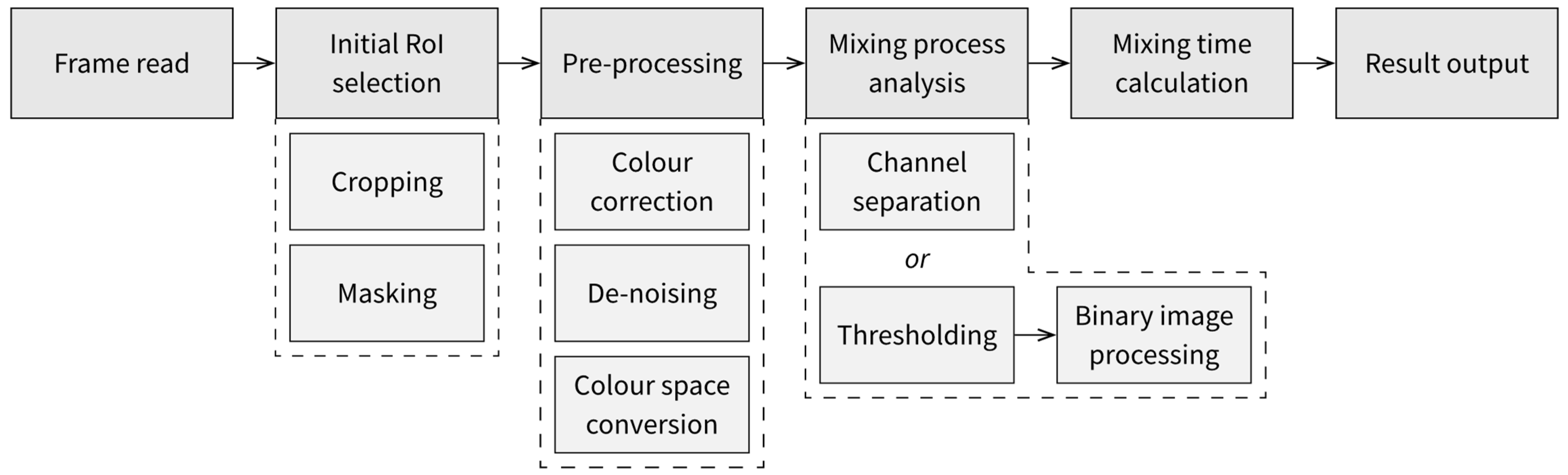
5.1. Processing Algorithm

After the video material has been obtained, it has to be processed to extract valuable data about the mixing process. Nowadays, with computers with high processing power, it is appropriate to process the material through an algorithm that performs operations (Figure 4) on every frame of the video material.

Every digital video file consists of digital still images called frames. Each frame has to be read before processing and stored in memory as a table with cells corresponding to each pixel containing the colour information (Figure 5). In some situations where the observed vessel is not stationary related to the camera, which could be the case, for example, with shaken vessels, only some frames could be selected for processing, such as those separated by a time interval corresponding to the shaking motion oscillation period.

After reading a frame, an initial region of interest (RoI) selection can be performed. Depending on the experimental setup and how the captured vessel is placed inside the camera field of view, the image can be cropped or masked so that only the parts representing the observed liquid remain for a further analysis. The masking can be performed manually and only once for a given setup if the apparent shape of the vessel and the agitating equipment is constant for the duration of the video and the camera’s position related to the filmed vessel is not changing between measurements (Figure 6). The masking can also be performed through thresholding, with selected parts of the vessel or the surroundings marked, for example, with a specific colour not interfering with the colour of the observed liquid. A combination of the two methods could also be used, for example, when minor movement of the camera occurs during the measurement, as could be with cameras mounted to the rocker in wave-mixed devices or to the oscillating platform in shaken devices.

With the appropriate region of interest selected, image processing can be performed to improve the quality of the data or make them suitable for further operations. The processing could involve colour corrections, such as contrast expansion, changes in white balance, brightness or gamma correction of the image [58]. Image processing can also involve operations to decrease noise, which can appear due to insufficient lighting in some parts of the image. The de-noising can be performed with filtering algorithms (e.g., Gaussian, median or bilateral) [59]. Image processing should be limited to as few operations as possible, as it will increase the amount of computational power necessary for the whole process. This goal can be achieved by obtaining high-quality video material, as described in Section 4.

Colour space conversion is an operation that can be performed to make the data easier to analyse, for example, by simplifying the selection of colours corresponding to mixed and unmixed regions. Choice of the colour space should be performed based on what colour-changing reagents are used during the experiments. For example, if bromothymol blue, which changes colour from blue to yellow, was to be used, the b* component of the L*a*b* space could be used for a simple selection of colour ranges corresponding to each state of the indicator. Colour spaces and their characteristics are explained in Section 5.2.

The approach taken during the analysis of the mixing process can be different depending on the characteristics of the observed vessel, what the liquid flow characteristics inside the observed vessel are and what definition of mixing time is intended to be used at the end of the process (see Section 5.3):

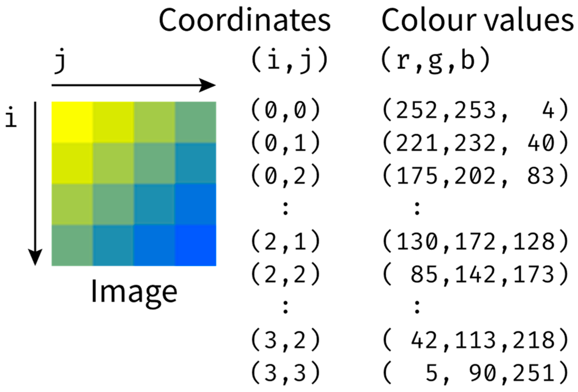
• The first approach to obtaining data about the mixing process is to perform separation of the image’s colour channels, select one of the components and directly observe changes in the values of the component, either averaged across the whole domain or divided into subdomains or individual pixels.
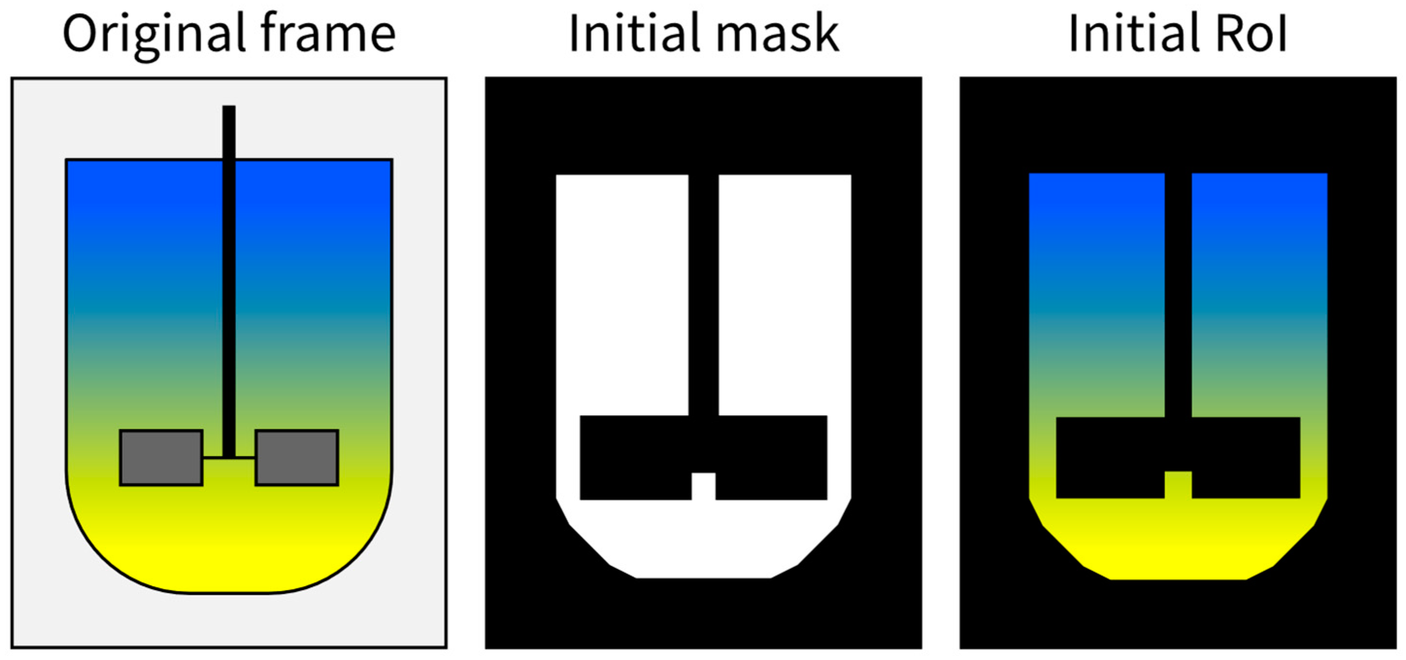
• The second approach, which could be used when the apparent shape of the observed liquid changes in time, is to find the areas corresponding to each discernible state of mixedness through thresholding. The thresholding will require the selection of colour ranges corresponding to each state of the applied indicators, which, if the video material is filmed at consistent filming parameters, should be performed once for the whole series of measurements. The binary masks resulting from thresholding can be improved with binary image operations, such as erosion and dilation or opening and closing [59].

5.2. Colour Spaces

A crucial point of an image analysis is determining how the colour information corresponds to the mixedness state of the liquid. The colour information is stored in the image with values organised according to a specified colour space. Multiple colour spaces have been developed, each varying in how they represent colour [60]. The following paragraphs contain brief descriptions of selected colour spaces, which were previously broadly adopted during colourimetric method studies or could be used more often given their utilisation in similar areas.

The grayscale is the simplest way of representing differences between areas of liquid differing in relative brightness, which has been utilised in colourimetric mixing time determination [26,31]. In grayscale, only information on the lightness of a pixel is stored. Usually, the single parameter of grayscale is limited from 0 (black) to 255 (white). Grayscale can be suited for analysing images in which the liquid’s initial and final colours differ strongly in brightness. However, since all other colour information is not preserved, it is recommended that other options be examined. The choice of colour space should be based on the available functionality in the software selected for the image processing and the effectiveness of colour separation assessed during the initial tests of the image processing algorithm.

RGB colour space (Figure 7, left) consists of three channels: R for the intensity of red colour in the image, G for green and B for blue. It is used in almost all popular digital output systems for everyday use [61]. Through its abundance, most papers regarding the colourimetric mixing time measurement method use RGB or some part of it to represent colour information. However, RGB has disadvantages, such as high correlation among its components [62] and being susceptible to changes in scene illumination [63].

HSV colour space (Figure 7, centre) consists of three channels: H for the hue of the colour, S for saturation and V for the value (intensity). The HSV space can be represented as a cylinder, in which the H channel is scaled as an angular component, the S channel corresponds to the radial dimension and the V channel is scaled in the axial dimension [60]. HSV space differs from RGB as it separates the information on the intensity of colour from the hue [64].

L*a*b* (Figure 7, right) is a colour space defined by the International Commission on Illumination, consisting of three channels: L* corresponds to the lightness of the colour, while a* and b* are chromatic components with negative and positive values for colour opponents. The a* component indicates where the colour falls along the red–green axis, and the b* component represents the position of colour on the blue–yellow axis [65]. L*a*b* colour space was designed to be uniform and is approximately linear, which means that a distance between two colours in L*a*b* space corresponds to a similar perceived difference for the observer [66]. It also provides good separation of the lightness component from the saturation and hue components [61]. L*a*b* is frequently used in food science [67,68], for human face detection applications [69] or in optoelectronics [70]. Trujillo-de Santiago et al. [71] presented results for mixing time measurements in a vessel filled with an opaque non-Newtonian blue maise flour suspension, which is an unusual example, given that the colour change could only be detected on the outer surface of the fluid.

5.3. Mixing Time Value Calculation

5.3.1. Global Mixing Time

Processing the video data should lead to obtaining data describing the mixing process inside the studied vessel. The simplest quantitative result, which can be obtained with the colourimetric method, is the global mixing time value. Different definitions of global mixing time have been used in different studies, the summary of which is presented below.

In the case of works where the liquid was observed visually, the mixing time was usually defined as the moment in which the last element of liquid in the colour representing the unmixed state has been eliminated [11,15]. Usually, indicators used during the experiments with visual observations had a dark and saturated colour in the unmixed state and were colourless or light-coloured in the final state. Therefore, the goal was to catch the point where the last dark-coloured spot in the liquid disappeared [12].

After the advent of a computer-aided image analysis, the global mixing time value definitions rely on specifying a measure of the progress of the observed process. In general, the parameter taken as the measure of mixing progress can be normalised to obtain a homogeneity $Ho$ value with the use of the following equation [72]:

$$Ho\left(t\right)=\frac{X_{\infty }-X\left(t\right)}{X_{\infty }-X\left(0\right)}$$

(1)

In Equation (1), X is the parameter taken as the measure of mixing progress, and $X\left(t\right)$ is the parameter value at the time $t$. $X\left(0\right)$ is the value of the parameter at the moment of tracer injection. $X_{\infty }$ is the value of the parameter at the end of the measurement after a steady state has been reached. Mixing time is then defined as the moment in time when $Ho$ permanently reaches 100% within some specified deviation, for example, 5% or 10%.

Delaplace et al. [18] have defined the mixing time as the time between tracer injection and the moment of achieving less than 10% deviation in the green channel brightness compared to the mean level. The green channel from RGB space has been used, as the increase in its values is related to the change in liquid colour from red to yellow, the latter being a mixture of the red and green components.

Cabaret et al. [10] examined which of the three RGB channels is most suitable for global mixing time determination based on the amplitude of change and the stability of values in the mixed state for the values of each channel. The authors specified which RGB component gives the best colour separation for several pH indicators. In the study of Cabaret et al., the mixing efficiency at a given moment is defined as a ratio between the number of pixels corresponding to the mixed liquid and the total number of pixels in the region of interest [10].

A different approach for global mixing time calculation has been used by Xiao et al. [44] and previously also by Trujillo-de Santiago et al. [71]. In these reports, the three colour values for each picture element are treated as Cartesian coordinates of points in 3D space. At any moment $t$, a distance between points represents the current colour of a given picture element and the final colour of mixed liquid. The distance, which then is taken as the measure of mixing progress, can be calculated according to the following expression:

$$D_{ij}\left(t\right)=\sqrt{{\left({\overline{K}}_{\infty }-K_{ij}\left(t\right)\right)}^2+{\left({\overline{L}}_{\infty }-L_{ij}\left(t\right)\right)}^2+{\left({\overline{M}}_{\infty }-M_{ij}\left(t\right)\right)}^2}$$

(2)

In Equation (2), $i$ and $j$ are the coordinates of a given pixel in the analysed image, $\left(K_{ij}\left(t\right), L_{ij}\left(t\right), M_{ij}\left(t\right)\right)$ are the colour values of the pixel in an arbitrary colour space at a given moment $t$, $\left({\overline{K}}_{\infty }, {\overline{L}}_{\infty }, M_{\infty }\right)$ are the colour values in the final homogenous state averaged across the whole analysed area and $D_{ij}\left(t\right)$ is the distance between those values represented by two points in 3D space.

The $D_{ij}\left(t\right)$ values for all pixels can be normalised with the use of Equation (1). The global mixing time can be calculated by averaging the homogeneity values across the whole picture domain and taking the time value at which a given deviation from 100% homogeneity is reached, analogously to the previously described method. The averaging of the homogeneity values can be performed by using an equation:

$$\overline{Ho}\left(t\right)=\frac{\sum _{ij}^{A}H{o}_{ij}\left(t\right)}{A}$$

(3)

$A$ in Equation (3) represents the area, i.e., the total number of pixels, assigned to the analysed region of interest. In the simplest case, with a rectangular region of interest, $A$ would be equal to the product of its width and height.

The mixing time value can also be determined through the analysis of the log root-mean-square variance of the normalised homogeneity values, as presented in studies of Gabelle et al. [24] and the report of Plais and Augier [43] based on the work of Brown et al. [8]:

$$\log {\sigma }_{RMS}^2=\log \left(\frac{1}{np}\sum _{i=1}^{np}{\left(Ho\left(t\right)-1\right)}^2\right)$$

(4)

In the work of Brown et al. [8], where this definition was intended for use with the sensor method, $np$ in Equation (4) represents the number of probes placed in the liquid. In the works of Gabelle et al. [24] and the study of Plais and Augier [43], $np$ corresponds to the number of subdivisions introduced into the original image. With this approach, mixing time with a 5% deviation from perfect homogeneity is defined as the moment when $\log {\sigma }_{RMS}^2=-2.6$.

5.3.2. Local Mixing Time, Mixing Time Maps

Apart from calculating global mixing time values, which can be performed using any mixing time measurement method, the colourimetric method offers the possibility of obtaining local mixing time values in any chosen area of the liquid. The main region of interest can be split into multiple parts, with the smallest possible being the single pixel of the original image. The local mixing time value can be calculated similarly to the global mixing time but without averaging homogeneity values across the entire analysed image.

Local mixing time values can be presented as mixing time maps. Mixing time maps can be prepared by mapping the local mixing time values to a colour scale and plotting them on a 2D surface in spots corresponding to the areas or pixels in the original frame. Mixing time maps can be a tool for easy quantification of compartments and concentration gradients during the mixing process and have been used to present data in studies regarding various types of vessels and colourimetric method variants [30,31,37,38,40,41,44].

5.4. Software Tools

There are several software tools available for the processing of obtained video material. Free and open-source software tools can be used over proprietary programs to improve reproducibility and decrease the cost of research. The selection of software used for image processing should also be based on the programming experience of the personnel and whether it provides all necessary functions.

The software that is frequently used for the image processing based on the data in Table 1 is MATLAB by The MathWorks, Inc. Many authors mention the use of this environment for the processing of image data [28,30,33] and for the further calculations of the mixing time value [26]. In some studies, the Image Processing Toolbox is mentioned [32], a part of the library of extensions to the MATLAB environment containing functions dedicated to image data operations. The popularity of MATLAB among researchers [73] and extensive user documentation may facilitate the implementation of this environment into research based on the colourimetric method.

Another piece of software used during the image analysis by some researchers [3,26,29] is ImageJ—an open-source application for batch processing of images developed at the National Institute of Health in the United States. It is mainly used in medical applications and supports image analysis functions, which can be expanded through plug-ins [74]. ImageJ is operated through a graphical user interface, which can make it more accessible for research teams. Detailed documentation for the program is available on the project’s website.

The OpenCV library provides tools for computer-vision-related tasks in many research and commercial applications [75]. It is free, open-source and available for Python and C++. The library has extensive functionality, containing numerous algorithms for accepting video streams, accessing pixel data and performing morphological and filtering operations, among others [76]. Similarly to the MATLAB Image Processing Toolbox, implementation of OpenCV will require moderate programming skills. Documentation, tutorials and other helpful resources are widely available without additional cost, which could enable researchers with some programming experience to use OpenCV in their research for analysing colourimetric method video material.

6. Conclusions

The colourimetric method is a powerful way of examining the mixing performance in tank reactors and various bioreactors. The application of the method has been well documented across systems varying in their working principle and characteristics, including the material of the vessel and the agitation mechanism employed. The colourimetric method allows for detailed observation of liquid flow during the mixing process in the whole body of liquid or with a focus on specifically selected areas inside the reactor, which gives it a substantial advantage over local sensor methods. The method is non-invasive, which enables the examination of liquid flow patterns in setups with various geometries and mixing mechanisms without unwanted disturbances and difficult-to-quantify errors resulting from introducing additional sensors or equipment into the vessel. It is possible to implement the colourimetric method approach with easily accessible chemicals (iodometry redox reaction or neutralisation reaction with pH indicators) and affordable equipment (widely available commercial cameras). The computerised analysis of the video material gathered through the experiments increases the interdisciplinarity of the studies, integrating bioreactor and fluid mechanics research with computer science. The wide availability of image analysis tools and multiple documented definitions for mixing time value calculation give flexibility and room for adjustment of the method for the requirements of a specific experimental setup. Additionally, a thorough analysis of the images can provide valuable information about the liquid flow patterns or zones with insufficient mixing inside the vessel. Broader application of the colourimetric method could accelerate the development of new bioreactor systems and the examination of their characteristics, including prototypical devices with newly developed geometries or agitation mechanisms.

References

1. Godleski, E.S.; Smith, J.C. Power Requirements and Blend Times in the Agitation of Pseudoplastic Fluids. AIChE J. 1962, 8, 617–620. [Google Scholar] [CrossRef]
2. Gaugler, L.; Mast, Y.; Fitschen, J.; Hofmann, S.; Schlüter, M.; Takors, R. Scaling-down Biopharmaceutical Production Processes via a Single Multi-compartment Bioreactor (SMCB). Eng. Life Sci. 2023, 23, e2100161. [Google Scholar] [CrossRef] [PubMed]
3. Rosseburg, A.; Fitschen, J.; Wutz, J.; Wucherpfennig, T.; Schlüter, M. Hydrodynamic Inhomogeneities in Large Scale Stirred Tanks—Influence on Mixing Time. Chem. Eng. Sci. 2018, 188, 208–220. [Google Scholar] [CrossRef]
4. Ascanio, G. Mixing Time in Stirred Vessels: A Review of Experimental Techniques. Chin. J. Chem. Eng. 2015, 23, 1065–1076. [Google Scholar] [CrossRef]
5. Hillig, F.; Pilarek, M.; Junne, S.; Neubauer, P. Cultivation of Marine Microorganisms in Single-Use Systems. In Disposable Bioreactors II; Eibl, D., Eibl, R., Eds.; Advances in Biochemical Engineering/Biotechnology; Springer: Berlin/Heidelberg, Germany, 2013; Volume 138, pp. 179–206. ISBN 978-3-642-45157-7. [Google Scholar]
6. Tan, R.-K.; Eberhard, W.; Büchs, J. Measurement and Characterization of Mixing Time in Shake Flasks. Chem. Eng. Sci. 2011, 66, 440–447. [Google Scholar] [CrossRef]
7. Li, L.; Wang, K.; Zhao, Q.; Gao, Q.; Zhou, H.; Jiang, J.; Mei, W. A Critical Review of Experimental and CFD Techniques to Characterize the Mixing Performance of Anaerobic Digesters for Biogas Production. Rev. Environ. Sci. Bio/Technol. 2022, 21, 665–689. [Google Scholar] [CrossRef]
8. Brown, D.A.R.; Jones, P.N.; Middleton, J.C.; Papadopoulos, G.; Arik, E.B. Experimental Methods. In Handbook of Industrial Mixing; Paul, E.L., Atiemo-Obeng, V.A., Kresta, S.M., Eds.; John Wiley & Sons Inc.: Hoboken, NJ, USA, 2003; pp. 145–256. ISBN 978-0-471-26919-9. [Google Scholar]
9. Löffelholz, C.; Husemann, U.; Greller, G.; Meusel, W.; Kauling, J.; Ay, P.; Kraume, M.; Eibl, R.; Eibl, D. Bioengineering Parameters for Single-Use Bioreactors: Overview and Evaluation of Suitable Methods. Chem. Ing. Tech. 2013, 85, 40–56. [Google Scholar] [CrossRef]
10. Cabaret, F.; Bonnot, S.; Fradette, L.; Tanguy, P.A. Mixing Time Analysis Using Colorimetric Methods and Image Processing. Ind. Eng. Chem. Res. 2007, 46, 5032–5042. [Google Scholar] [CrossRef]
11. Fox, E.A.; Gex, V.E. Single-Phase Blending of Liquids. AIChE J. 1956, 2, 539–544. [Google Scholar] [CrossRef]
12. Norwood, K.W.; Metzner, A.B. Flow Patterns and Mixing Rates in Agitated Vessels. AIChE J. 1960, 6, 432–437. [Google Scholar] [CrossRef]
13. Carreau, P.J.; Patterson, I.; Yap, C.Y. Mixing of Viscoelastic Fluids with Helical-Ribbon Agitators. I—Mixing Time and Flow Patterns. Can. J. Chem. Eng. 1976, 54, 135–142. [Google Scholar] [CrossRef]
14. Haß, V.C.; Nienow, A.W. Ein Neuer, Axial Fördernder Rührer Zum Dispergieren von Gas in Flüssigkeiten: Ein Neuer, Axial Fördernder Rührer Zum Dispergieren von Gas in Flüssigkeiten. Chem. Ing. Tech. 1989, 61, 152–154. [Google Scholar] [CrossRef]
15. Saito, F.; Nienow, A.W.; Chatwin, S.; Moore, I.P.T. Power, Gas Dispersion and Homogenisation Characteristics of Scaba SRGT and Rushton Turbine Impellers. J. Chem. Eng. Jpn. JCEJ 1992, 25, 281–287. [Google Scholar] [CrossRef]
16. Lamberto, D.J.; Muzzio, F.J.; Swanson, P.D.; Tonkovich, A.L. Using Time-Dependent RPM to Enhance Mixing in Stirred Vessels. Chem. Eng. Sci. 1996, 51, 733–741. [Google Scholar] [CrossRef]
17. Kraume, M.; Zehner, P. Experience with Experimental Standards for Measurements of Various Parameters in Stirred Tanks. Chem. Eng. Res. Des. 2001, 79, 811–818. [Google Scholar] [CrossRef]
18. Delaplace, G.; Bouvier, L.; Moreau, A.; Guérin, R.; Leuliet, J.-C. Determination of Mixing Time by Colourimetric Diagnosis—Application to a New Mixing System. Exp. Fluids 2004, 36, 437–443. [Google Scholar] [CrossRef]
19. Foucault, S.; Ascanio, G.; Tanguy, P.A. Mixing Times in Coaxial Mixers with Newtonian and Non-Newtonian Fluids. Ind. Eng. Chem. Res. 2006, 45, 352–359. [Google Scholar] [CrossRef]
20. Bonnot, S.; Cabaret, F.; Fradette, L.; Tanguy, P.A. Characterization of Mixing Patterns in a Coaxial Mixer. Chem. Eng. Res. Des. 2007, 85, 1129–1135. [Google Scholar] [CrossRef]
21. Delaplace, G.; Thakur, R.K.; Bouvier, L.; André, C.; Torrez, C. Dimensional Analysis for Planetary Mixer: Mixing Time and Reynolds Numbers. Chem. Eng. Sci. 2007, 62, 1442–1447. [Google Scholar] [CrossRef]
22. Fradette, L.; Thomé, G.; Tanguy, P.A.; Takenaka, K. Power and Mixing Time Study Involving a Maxblend® Impeller with Viscous Newtonian and Non-Newtonian Fluids. Chem. Eng. Res. Des. 2007, 85, 1514–1523. [Google Scholar] [CrossRef]
23. Iranshahi, A.; Devals, C.; Heniche, M.; Fradette, L.; Tanguy, P.A.; Takenaka, K. Hydrodynamics Characterization of the Maxblend Impeller. Chem. Eng. Sci. 2007, 62, 3641–3653. [Google Scholar] [CrossRef]
24. Gabelle, J.-C.; Augier, F.; Carvalho, A.; Rousset, R.; Morchain, J. Effect of Tank Size on k L a and Mixing Time in Aerated Stirred Reactors with Non-newtonian Fluids. Can. J. Chem. Eng. 2011, 89, 1139–1153. [Google Scholar] [CrossRef]
25. Sieblist, C.; Jenzsch, M.; Pohlscheidt, M.; Lübbert, A. Insights into Large-Scale Cell-Culture Reactors: I. Liquid Mixing and Oxygen Supply. Biotechnol. J. 2011, 6, 1532–1546. [Google Scholar] [CrossRef] [PubMed]
26. Allonneau, C.; Olmos, E.; Guyot, S.; Ferret, E.; Gervais, P.; Cachon, R. Hydrodynamic Characterization of a New Small-Scale Reactor Mixed by a Magnetic Bar. Biochem. Eng. J. 2015, 96, 29–37. [Google Scholar] [CrossRef]
27. Trad, Z.; Fontaine, J.-P.; Larroche, C.; Vial, C. Experimental and Numerical Investigation of Hydrodynamics and Mixing in a Dual-Impeller Mechanically-Stirred Digester. Chem. Eng. J. 2017, 329, 142–155. [Google Scholar] [CrossRef]
28. Chezeau, B.; Fontaine, J.P.; Vial, C. Analysis of Liquid-to-Gas Mass Transfer, Mixing and Hydrogen Production in Dark Fermentation Process. Chem. Eng. J. 2019, 372, 715–727. [Google Scholar] [CrossRef]
29. Amiraftabi, M.; Khiadani, M.; Mohammed, H.A. Performance of a Dual Helical Ribbon Impeller in a Two-Phase (Gas-Liquid) Stirred Tank Reactor. Chem. Eng. Process. Process Intensif. 2020, 148, 107811. [Google Scholar] [CrossRef]
30. Samaras, J.J.; Ducci, A.; Micheletti, M. Flow, Suspension and Mixing Dynamics in DASGIP Bioreactors, Part 2. AIChE J. 2020, 66, e16999. [Google Scholar] [CrossRef]
31. Fitschen, J.; Hofmann, S.; Wutz, J.; Kameke, A.V.; Hoffmann, M.; Wucherpfennig, T.; Schlüter, M. Novel Evaluation Method to Determine the Local Mixing Time Distribution in Stirred Tank Reactors. Chem. Eng. Sci. X 2021, 10, 100098. [Google Scholar] [CrossRef]
32. Vivek, V.; Eka, F.N.; Chew, W. Mixing Studies in an Unbaffled Bioreactor Using a Computational Model Corroborated with In-Situ Raman and Imaging Analyses. Chem. Eng. J. Adv. 2022, 9, 100232. [Google Scholar] [CrossRef]
33. Tregidgo, M.; Dorn, M.; Lucas, C.; Micheletti, M. Design and Characterization of a Novel Perfusion Reactor for Biopharmaceuticals Production. Chem. Eng. Res. Des. 2023, 194, 344–357. [Google Scholar] [CrossRef]
34. Kaiser, S.C.; Eibl, R.; Eibl, D. Engineering Characteristics of a Single-Use Stirred Bioreactor at Bench-Scale: The Mobius CellReady 3L Bioreactor as a Case Study. Eng. Life Sci. 2011, 11, 359–368. [Google Scholar] [CrossRef]
35. Nienow, A.W.; Rielly, C.D.; Brosnan, K.; Bargh, N.; Lee, K.; Coopman, K.; Hewitt, C.J. The Physical Characterisation of a Microscale Parallel Bioreactor Platform with an Industrial CHO Cell Line Expressing an IgG4. Biochem. Eng. J. 2013, 76, 25–36. [Google Scholar] [CrossRef]
36. Delbridge, J.N.; Barrett, T.A.; Ducci, A.; Micheletti, M. Power, Mixing and Flow Dynamics of the Novel AllegroTM Stirred Tank Reactor. Chem. Eng. Sci. 2023, 271, 118545. [Google Scholar] [CrossRef]
37. Tissot, S.; Farhat, M.; Hacker, D.L.; Anderlei, T.; Kühner, M.; Comninellis, C.; Wurm, F. Determination of a Scale-up Factor from Mixing Time Studies in Orbitally Shaken Bioreactors. Biochem. Eng. J. 2010, 52, 181–186. [Google Scholar] [CrossRef]
38. Monteil, D.T.; Tontodonati, G.; Ghimire, S.; Baldi, L.; Hacker, D.L.; Bürki, C.A.; Wurm, F.M. Disposable 600-mL Orbitally Shaken Bioreactor for Mammalian Cell Cultivation in Suspension. Biochem. Eng. J. 2013, 76, 6–12. [Google Scholar] [CrossRef]
39. Werner, S.; Greulich, J.; Geipel, K.; Steingroewer, J.; Bley, T.; Eibl, D. Mass Propagation of Helianthus annuus Suspension Cells in Orbitally Shaken Bioreactors: Improved Growth Rate in Single-Use Bag Bioreactors. Eng. Life Sci. 2014, 14, 676–684. [Google Scholar] [CrossRef]
40. Rodriguez, G.; Anderlei, T.; Micheletti, M.; Yianneskis, M.; Ducci, A. On the Measurement and Scaling of Mixing Time in Orbitally Shaken Bioreactors. Biochem. Eng. J. 2014, 82, 10–21. [Google Scholar] [CrossRef]
41. Rodriguez, G.; Micheletti, M.; Ducci, A. Macro- and Micro-Scale Mixing in a Shaken Bioreactor for Fluids of High Viscosity. Chem. Eng. Res. Des. 2018, 132, 890–901. [Google Scholar] [CrossRef]
42. Jones, S.M.J.; Louw, T.M.; Harrison, S.T.L. Energy Consumption Due to Mixing and Mass Transfer in a Wave Photobioreactor. Algal Res. 2017, 24, 317–324. [Google Scholar] [CrossRef]
43. Plais, C.; Augier, F. Effect of Liquid Viscosity on Mixing Times in Bubble Columns. Theor. Found. Chem. Eng. 2016, 50, 969–974. [Google Scholar] [CrossRef]
44. Xiao, J.; Zou, C.; Liu, M.; Zhang, G.; Delaplace, G.; Jeantet, R.; Chen, X.D. Mixing in a Soft-Elastic Reactor (SER) Characterized Using an RGB Based Image Analysis Method. Chem. Eng. Sci. 2018, 181, 272–285. [Google Scholar] [CrossRef]
45. Wurm, H.; Sandmann, M. Establishment of a Simple Method to Evaluate Mixing Times in a Plastic Bag Photobioreactor Using Image Processing Based on Freeware Tools. BMC Res. Notes 2021, 14, 470. [Google Scholar] [CrossRef] [PubMed]
46. Hoogendoorn, C.J.; Den Hartog, A.P. Model Studies on Mixers in the Viscous Flow Region. Chem. Eng. Sci. 1967, 22, 1689–1699. [Google Scholar] [CrossRef]
47. Bartczak, M.; Wierzchowski, K.; Pilarek, M. Mixing Performance in a Litre-Scale Rocking Disposable Bioreactor: DoE-Based Investigation of Mixing Time Dependence on Operational Parameters. Chem. Eng. J. 2022, 431, 133288. [Google Scholar] [CrossRef]
48. Guillard, F.; Trägårdh, C.; Fuchs, L. A Study of Turbulent Mixing in a Turbine-Agitated Tank Using a Fluorescence Technique. Exp. Fluids 2000, 28, 225–235. [Google Scholar] [CrossRef]
49. Paul, E.L.; Atiemo-Obeng, V.A.; Kresta, S.M. (Eds.) Handbook of Industrial Mixing: Science and Practice; Wiley-Interscience: Hoboken, NJ, USA, 2004; ISBN 978-0-471-26919-9. [Google Scholar]
50. Melton, L.A.; Lipp, C.W.; Spradling, R.W.; Paulson, K.A. Dismt—Determination of Mixing Time through Color Changes. Chem. Eng. Commun. 2002, 189, 322–338. [Google Scholar] [CrossRef]
51. Vanhamel, S.; Masy, C. Production of Disposable Bags: A Manufacturer’s Report. In Single-Use Technology in Biopharmaceutical Manufacture; Eibl, R., Eibl, D., Eds.; John Wiley & Sons Inc.: Hoboken, NJ, USA, 2011; pp. 113–134. ISBN 978-0-470-90999-7. [Google Scholar]
52. Alvarez, M.M.; Guzmán, A.; Elías, M. Experimental Visualization of Mixing Pathologies in Laminar Stirred Tank Bioreactors. Chem. Eng. Sci. 2005, 60, 2449–2457. [Google Scholar] [CrossRef]
53. Vega-Alvarado, L.; Taboada, B.; Hidalgo-Millán, A.; Ascanio, G. An Image Analysis Method for the Measurement of Mixing Times in Stirred Vessels. Chem. Eng. Technol. 2011, 34, 859–866. [Google Scholar] [CrossRef]
54. Seletzky, J.; Otten, K.; Lotter, S.; Fricke, J.; Peter, C.; Maier, H.; Büchs, J. A Simple and Inexpensive Method for Investigating Microbiological, Enzymatic, or Inorganic Catalysis Using Standard Histology and Microbiology Laboratory Equipment: Assembly, Mass Transfer Properties, Hydrodynamic Conditions and Evaluation. Biotech. Histochem. 2006, 81, 133–138. [Google Scholar] [CrossRef]
55. Jossen, V.; Eibl, R.; Eibl, D. Single-Use Bioreactors—An Overview. In Single-Use Technology in Biopharmaceutical Manufacture; Eibl, R., Eibl, D., Eds.; John Wiley & Sons Ltd.: Hoboken, NJ, USA, 2019; pp. 37–52. ISBN 978-1-119-47789-1. [Google Scholar]
56. Bartczak, M.; Wierzchowski, K.; Pilarek, M. Mass Transfer in a Liter-Scale Wave Mixed Single-Use Bioreactor: Influence of Viscosity and Antifoaming Agent. Ind. Eng. Chem. Res. 2023, 62, 10893–10902. [Google Scholar] [CrossRef]
57. Sharma, R.; Collair, W.; Williams, A.; Harrison, S.T.L.; Tai, S.L. Design and Engineering Characterization of a Horizontal Tubular Bioreactor with Spiral Impeller for Cell Cultivation. Biochem. Eng. J. 2023, 191, 108794. [Google Scholar] [CrossRef]
58. Burger, W.; Burge, M.J. Digital Image Processing: An Algorithmic Introduction Using Java; Texts in Computer Science; Springer: London, UK, 2008; ISBN 978-1-84628-379-6. [Google Scholar]
59. Russ, J.C. The Image Processing Handbook; CRC Press: Boca Raton, FL, USA, 2006; ISBN 978-0-203-88109-5. [Google Scholar]
60. Tkalcic, M.; Tasic, J.F. Colour Spaces: Perceptual, Historical and Applicational Background. In Proceedings of the The IEEE Region 8 EUROCON 2003. Computer as a Tool, Ljubljana, Slovenia, 22–24 September 2003; IEEE: Ljubljana, Slovenia, 2003; Volume 1, pp. 304–308. [Google Scholar]
61. Kahu, S.Y.; Raut, R.B.; Bhurchandi, K.M. Review and Evaluation of Color Spaces for Image/Video Compression. Color Res. Appl. 2019, 44, 8–33. [Google Scholar] [CrossRef]
62. Cheng, H.D.; Jiang, X.H.; Sun, Y.; Wang, J. Color Image Segmentation: Advances and Prospects. Pattern Recognit. 2001, 34, 2259–2281. [Google Scholar] [CrossRef]
63. Liu, Y.; Yang, F.; Yang, R.; Jia, K.; Zhang, H. Research on Segmentation of Weed Images Based on Computer Vision. J. Electron. 2007, 24, 285–288. [Google Scholar] [CrossRef]
64. Sural, S.; Qian, G.; Pramanik, S. Segmentation and Histogram Generation Using the HSV Color Space for Image Retrieval. In Proceedings of the International Conference on Image Processing, Rochester, NY, USA, 22–25 September 2002; IEEE: Rochester, NY, USA, 2002; Volume 2, pp. II-589–II-592. [Google Scholar]
65. Bora, D.J.; Gupta, A.K.; Khan, F.A. Comparing the Performance of L*A*B* and HSV Color Spaces with Respect to Color Image Segmentation. arXiv 2015, arXiv:1506.01472. [Google Scholar] [CrossRef]
66. Alata, O.; Quintard, L. Is There a Best Color Space for Color Image Characterization or Representation Based on Multivariate Gaussian Mixture Model? Comput. Vis. Image Underst. 2009, 113, 867–877. [Google Scholar] [CrossRef]
67. Lee, S.-M.; Lee, K.-T.; Lee, S.-H.; Song, J.-K. Origin of Human Colour Preference for Food. J. Food Eng. 2013, 119, 508–515. [Google Scholar] [CrossRef]
68. Afshari-Jouybari, H.; Farahnaky, A. Evaluation of Photoshop Software Potential for Food Colorimetry. J. Food Eng. 2011, 106, 170–175. [Google Scholar] [CrossRef]
69. Cai, J.; Goshtasby, A. Detecting Human Faces in Color Images. Image Vis. Comput. 1999, 18, 63–75. [Google Scholar] [CrossRef]
70. Suzuki, K.; Hirayama, E.; Sugiyama, T.; Yasuda, K.; Okabe, H.; Citterio, D. Ionophore-Based Lithium Ion Film Optode Realizing Multiple Color Variations Utilizing Digital Color Analysis. Anal. Chem. 2002, 74, 5766–5773. [Google Scholar] [CrossRef]
71. Trujillo-de Santiago, G.; Rojas-de Gante, C.; García-Lara, S.; Ballescá-Estrada, A.; Alvarez, M.M. Studying Mixing in Non-Newtonian Blue Maize Flour Suspensions Using Color Analysis. PLoS ONE 2014, 9, e112954. [Google Scholar] [CrossRef]
72. Bauer, I.; Dreher, T.; Eibl, D.; Glöckler, R.; Husemann, U.; John, G.T.; Kaiser, S.C.; Kampeis, P.; Kauling, J.; Kleebank, S.; et al. Recommendations for Process Engineering Characterisation of Single-Use Bioreactors and Mixing Systems by Using Experimental Methods, 2nd ed.; Dechema Biotechnologie: Frankfurt am Main, Germany, 2020; ISBN 978-3-89746-227-4. [Google Scholar]
73. Kong, J.; Dimitrov, M.; Yang, Y.; Liyanage, J.; Cao, L.; Staples, J.; Mantor, M.; Zhou, H. Accelerating MATLAB Image Processing Toolbox Functions on GPUs. In Proceedings of the 3rd Workshop on General-Purpose Computation on Graphics Processing Units, Pittsburgh, PA, USA, 14 March 2010; ACM: Pittsburgh, PA, USA, 2010; pp. 75–85. [Google Scholar]
74. Abràmoff, M.D.; Magalhães, P.J.; Ram, S.J. Image Processing with ImageJ. Biophotonics Int. 2004, 11, 36–42. [Google Scholar]
75. Culjak, I.; Abram, D.; Pribanic, T.; Dzapo, H.; Cifrek, M. A Brief Introduction to OpenCV. In Proceedings of the 2012 Proceedings of the 35th International Convention MIPRO, Opatija, Croatia, 21–25 May 2012; IEEE: Opatija, Croatia, 2012. [Google Scholar]
76. Howse, J. OpenCV Computer Vision with Python; Packt Publishing: Birmingham, UK, 2013; ISBN 978-1-78216-392-3. [Google Scholar]
Figure 1. pH colour change ranges of several indicators or systems of indicator used in colourimetric method applications.
Energies 17 00221 g001
Figure 2. Typical laboratory procedure for mixing time determination using the colourimetric method.
Energies 17 00221 g002
Figure 3. Example of the camera placement in a stirred tank setup with a lighting panel mounted behind the vessel for uniform illumination.
Energies 17 00221 g003
Figure 4. A scheme of suggested operations in an image processing algorithm for mixing time calculation with the colourimetric method. The main steps can be split into sub-operations performed as needed based on the form and quality of the initial video material and the selected definition for mixing time calculation.
Energies 17 00221 g004
Figure 5. Example of an image being represented as a table of values. Each pixel is assigned a set of coordinates (i, j), to which a triplet of values representing the colour information is attached. In the example, a gradient of yellow to blue across the diagonal of the image, the r and g values, which in combination represent the yellow colour, are getting smaller as the coordinate values increase. On the contrary, the b channel increases across the diagonal in accordance with the intensity of blue colour in the image. More information about the RGB colour space and other colour spaces is provided in Section 5.2.
Energies 17 00221 g005
Figure 6. An example of initial region of interest selection. A binary mask is constructed, which excludes the elements of a frame, which interfere with the observation of vessel contents. The mask is overlaid on top of the original frame to obtain an image for further processing.
Energies 17 00221 g006
Figure 7. Components of RGB, HSV and L*a*b* colour spaces with their typical ranges. Values of the other two components set for each axis are listed below their symbol. Values of RGB and HSV components are defined with numerical limits. In the case of the L*a*b* colour space, the values of the a* and b* components are theoretically unlimited. The limits in the graphic are typical for when 8-bit integer math is used.
Energies 17 00221 g007