Review

Review of Energy-Related Machine Learning Applications in Drying Processes

by
Damir Đaković
,
Miroslav Kljajić
*,
Nikola Milivojević
,
Đorđije Doder
and
Aleksandar S. Anđelković
Department of Energy and Process Engineering, Faculty of Technical Sciences, University of Novi Sad, 21000 Novi Sad, Serbia
*
Author to whom correspondence should be addressed.
Energies 2024, 17(1), 224; https://doi.org/10.3390/en17010224
Submission received: 29 November 2023 / Revised: 25 December 2023 / Accepted: 28 December 2023 / Published: 31 December 2023
(This article belongs to the Section K: State-of-the-Art Energy Related Technologies)

Abstract

:
Drying processes are among the most energy-intensive industrial processes. There is a need for development of the efficient methods needed for estimating, measuring, and reducing energy use. Different machine learning algorithms might provide some of the answers to these issues in a faster and less costly way, without the need for time-consuming and expensive experiments done at different scales of the dryers. The aim of this paper was to provide a comprehensive overview of machine learning applications for addressing energy-related challenges by exploration of different energy types and energy reduction opportunities. Also, the analysis of the applied algorithms, their specific applications and a critical evaluation of the obtained results are provided. The paper is based on the necessity of the improvements in energy use needed for drying related on the existing data. The overview of the ways for such achievements, and a general classification of machine learning algorithm are the background of the paper. The methods used are the machine learning techniques employed in different energy-related issues for drying processes. The paper focuses on the applications of artificial neural networks and other machine learning algorithms and models for different energy-related issues, including different energy types applications, challenges associated with energy consumption, and opportunities for energy reduction. Not only the applied algorithms, but also their specific applications, and the statistical analysis of the obtained results are also overviewed. Finally, a critical evaluation of the findings highlighting the potentials of machine learning algorithms in addressing energy-related challenges (such as estimation of energy consumption, opportunities for energy reduction, and use of different energy sources) is provided. The presented analysis underscored the effectiveness of machine learning applications for these purposes.

1. Introduction

There are a vast number of drying processes. In ref. [1], more than 15 various dryer types and 28 different industrial sectors are listed. This serves to underscore the significance of industrial drying, as evidenced by estimates that “show that 12–25% of the national industrial energy consumption in developed countries is attributed to industrial drying” [2]. Furthermore, the same source [2] reveals the potential for substantial energy savings, with expectations of energy savings of up to 80%, a 75% decrease in CO2 emissions, and a 20%/kg reduction in cost per kilogram of product through the utilization of heat pumps. Consequently, researchers in the field of drying have been and continue to be deeply concerned with improving drying processes and exploring alternative energy sources for dryers.
There are three primary ways for achieving an energy consumption reduction [3]:
evaporation load reduction, which can be accomplished by minimizing the initial moisture content or by avoiding over-drying;
enhancement of the dryer efficiency by reducing heat losses, implementing heat recovery, or changing operating parameters;
improving the energy supply utility system through the strategies of increasing boiler efficiency, reducing distribution losses, adopting combined heat and power (CHP) systems, incorporating heat pumps, utilizing waste incineration, or exploring low-cost fuel alternatives.
The emergence of artificial intelligence (AI) and its subfields has had a profound impact on various aspects of life, including prediction and identification of optimization possibilities in diverse industries. Machine learning (ML), a subset of AI (although the terms are sometimes used interchangeably) was first defined by A.L. Samuel in 1959 as follows: “Machine learning is the field of study that gives computers the ability to learn without being explicitly programmed” [4]. Notably, one of the earliest papers addressing machine learning algorithms in the context of drying was in ref. [5]. To the best of the authors’ knowledge, there were no previous overviews of this niche, although different reviews of drying, as well as the applications of machine learning in drying (mainly focused on food, but also on the pharmaceutical and bioprocessing industries) [6,7,8] were conducted.
Our research focuses on energy-related aspects of drying processes, encompassing various industries and commonly applied energy sources for drying, such as solar energy and heat pumps. There are four main types of machine learning algorithms: supervised, unsupervised, semi-supervised, and reinforcement learning.
Supervised learning algorithms use labeled datasets to make predictions. They are useful when the kind of outcome is known. The learning process is established by comparing predicted results with the actual results of input data (known as training data) and continuously adjusting the predictive model until the expected accuracy is reached.
There are three subtypes of supervised algorithms: classification, regression, and forecasting. Classification is used to determine, based on observed values, the category to which new observations belong. Regression is used for prediction and forecasting. The algorithms must estimate relationships between the variables (focus on one dependent variable and a series of changing variables). The algorithms used are include decision trees, Bayesian classification, least squares regression, logistic regression, support vector machines, and neural networks.
Unsupervised learning input data are not labeled. Extraction of general rules of the input data (through a mathematical process to systematically reduce redundancy or use similarity to organize data) is used for model preparation (clustering, dimensionality reduction, and association rule learning). The algorithms used are a priori and K-mean.
Semi-supervised learning input data are both labeled and unlabeled. They represent an extension of supervised learning. The model must be able to learn the structure in order to both organize the data and to make predictions (classification and regression). The algorithms used include graph theory inference algorithms and Laplacian support vector machines.
Reinforcement learning input data provide feedback to the model, emphasizing how to act based on the environment in order to provide maximization of the expected benefits. It does not require the correct input/output pairs or precise correction of sub-optimal behavior, as is the case in supervised learning. Reinforcement learning requires a balance between exploration in the unknown and compliance with existing knowledge. The algorithms used include Monte Carlo, Q-Learning, Deep Q-Networks (DQNs), policy gradient methods, PPO (proximal policy optimization), actor–critic, A2C (advantage actor–critic), TRPO (trust region policy optimization), A3C (asynchronous advantage actor–critic), DDPG (deep deterministic policy gradient), SAC (soft actor–critic), TD (temporal difference) learning, SARSA, DQL (Deep Q-Learning), D4PG (distributed distributional deterministic policy gradients), Rainbow, Ape-X, HER (Hindsight Experience Replay), model-based reinforcement learning, and AlphaZero. Machine learning algorithms can also be classified in other ways (e.g., by similarity of how they work).
A number of papers have analyzed ranges, from the general to a specific application related to only some specific aspects of energy use, such as forecasting of electric energy consumption [9], or to highly specialized works based on similarities and details of the interaction inside the biological neural networks [10].

2. Methodology

Different combinations of keywords were used (including, but not limited to “energy” and “drying” keywords, along with commonly used Boolean operators) in order to perform the searches and obtain the most relevant results. The search results were reviewed and irrelevant results were omitted. Only articles and review articles were taken into consideration, while conference papers, books, editorials, and similar were excluded (except for the explanations when groundbreaking references were included regardless of the type). The results shown in the paper were mostly published within the last 3 years (2020–2023), since the newest and the most comprehensive reviews were published in 2015, 2018, and 2019 [6,7,8]. Beside these, there are a few older references cited in relation to some historical beginnings of the relevant fields and general literature for both drying [1] and machine learning.
The basic methodologies for several of the algorithms most commonly used in drying applications are provided below.

2.1. Decision Tree

The decision tree algorithm is a machine learning algorithm. It can be used for classification and regression tasks. The basic idea of decision trees was first introduced by Ross Quinlan [11]. Later he developed the ID3 (Iterative Dichotomiser 3) algorithm [12], which was a specific implementation of a decision tree algorithm that used a top-down, greedy approach for tree construction by selecting the best attribute to split the data at each node. Later, there have been various extensions and improvements which were made to the basic algorithm (e.g., C4.5 and CART).
The decision tree algorithm recursively partitions the data into subsets based on the values of the input features, with the goal of creating homogeneous subsets that are easy to predict. The main steps and the structure of Decision Tree are:
  • The construction of a tree is done by the algorithm using a recursive partitioning of the data into the subsets based on the values of the input features. At each node of the tree, the algorithm selects the best feature to split the data based on a criterion (e.g. information gain or Gini impurity).
  • The splitting of the decision tree algorithm data is being continued until a stopping criterion is reached. It can be a maximum tree depth, a minimum number of samples per leaf node, or a minimum information gain.
  • After the construction of the tree, the algorithm can be used to predict new instances. Root node of the tree is a start point for prediction making. Then the decision rules are followed until a leaf node is reached, which label or value is then considered to be the prediction.
  • The missing values in the input features can be handled by using various strategies (e.g., surrogate splits, which use alternative features to make the decision, or imputation of the missing values based on the values of other features).
  • Regularization of the algorithm can be done by pruning the tree. It is done in order to remove unnecessary branches, which is the way to prevent overfitting and to reduce the complexity of the model.
  • The hyperparameters which can be tuned in order to optimize the performance of the algorithm are: the maximum tree depth, the minimum number of samples per leaf node, and the criterion used for splitting the data.
Input: Training data (X, y)
Tree Construction: Select the best feature for data splitting based on a criterion (e.g., information gain or Gini impurity);
Recursive partitioning of the data into the subsets based on the values of the input features;
Stop when a stopping criterion is met.
Prediction: Start at the root node of the tree;
Follow the decision rules until reaching a leaf node;
Use the label or value at the leaf node as the prediction.
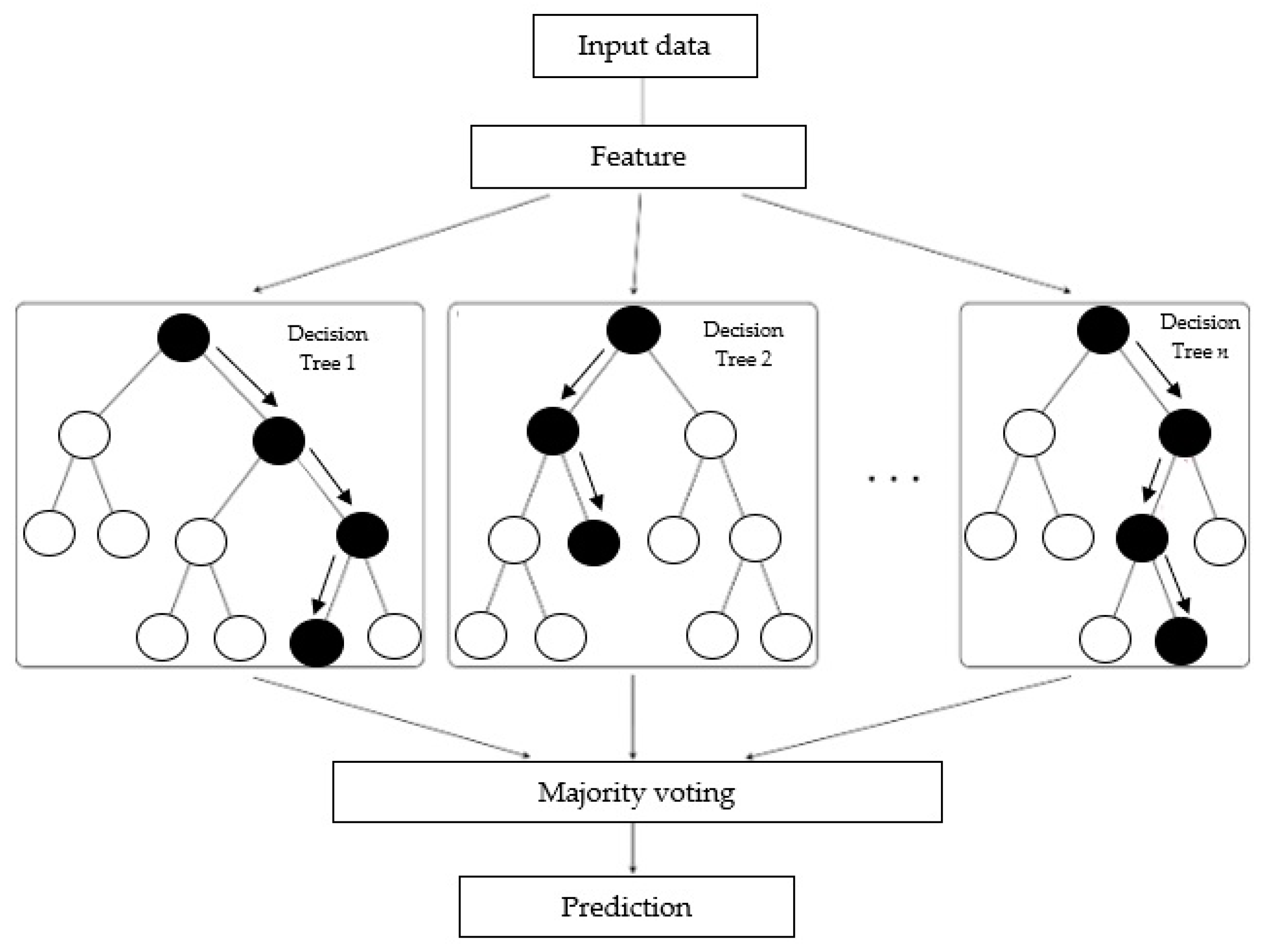
Handling Missing Values: Use surrogate splits or impute missing values based on the values of other features.
Regularization: Prune the tree to remove unnecessary branches.
Hyperparameter Tuning: Tune the hyperparameters of the decision tree algorithm to optimize the performance.

2.2. Random Forest

The random forest algorithm is a type of the decision tree algorithm. It combines multiple decision trees for the accuracy and robustness of the predictions improvement (ensemble algorithm). The first introduction of this algorithm was in 2001 by Leo Breiman [13]. It uses randomness for construction of a diverse set of decision trees, which can be combined in order to provide more accurate predictions. In the random forest algorithm, a large number of decision trees are trained on random subsets of the training data. Different subset is used for training each of the trees. The final prediction is made as a product of the aggregation of the predictions of all of the trees. It can be majority vote for classification, or averaging the predictions for regression type.
The steps of the random forest algorithm are:
  • Random forest uses a technique called bagging (bootstrap aggregating) for creation of a collection of the decision trees. It involves multiple random subsets of the training data creation, and training a decision tree on each subset. Averaging of the predictions of all the trees results in the final prediction.
  • A random subset of the input features which could be considered to be the best split is selected by the algorithm at each node of each decision tree. This is the way to improve the overall model performance and to help reduction of the correlation among the trees.
  • In order to provide a prediction, random forest calculates the average prediction of all the decision trees (for regression tasks), or takes a majority vote (for classification tasks).
  • Handling of the missing values in input features can be fulfilled through different strategies, either by so called surrogate splits or imputation of the missing values based on the values of other features.
  • Regularization of random forest can be done by tuning the hyperparameters. They can be, e.g., the number of the trees in the forest, the maximum tree depth, and the number of features to consider at each node.
  • There hyperparameters can be, also, tuned for optimization of the performance of the algorithm’s performance.
In Figure 1 is presented the random forest algorithm consisting of two decision trees that are used for data classification.

2.3. Support Vector Machine (SVM)

Support vector machine is a supervised algorithm. It can be used for regression and classification tasks (Figure 2 and Figure 3). The algorithm was made and promoted by Vapnik and his colleagues [14,15].
There are three main steps that make up SVM:
  • Kernel function calculation: the kernel function is calculated because it maps the input data into a higher-dimensional space in which is easier to find a hyperplane that separates the data into different classes.
  • The hyperplane that maximally separates the data into different classes is found. The hyperplane is chosen in that way that it has the largest distance to the nearest data point from each class.
  • The hyperplane is the base for the prediction of the algorithm.

2.4. Support Vector Regression (SVR)

Support vector regression is a machine learning algorithm used for regression tasks. It is a variant of SVM. SVR seeks a regression model with a margin close to the predicted values (Figure 4). It makes a balance between data fitting and overfitting avoiding.
These are the main steps of the SVR algorithm (Figure 5):
  • Kernel function is calculated. It maps input data into a higher-dimensional space. It is done because it is easier there to find a hyperplane which approximates the data.
  • The hyperplane approximating the data with the smallest error is found.
  • The hyperplane is the base for the prediction of the algorithm.
  • The error between the predicted and true values is calculated.
  • The hyperplane is updated based on the calculated error.

2.5. k-Nearest Neighbors (kNN)

k-nearest neighbors was introduced by several authors starting in the 1950s [16,17]. The algorithm consists of four main steps (Figure 6):
  • Calculation of the distance between the input data and all the training data.
  • K training data points that are closest to the input data are selected.
  • The output based on the K-nearest neighbors is calculated (if the kNN algorithm is used for classification, the class having the most representatives among the K-nearest neighbors will be predicted).
  • Finally, a prediction based on the calculated output is made.

2.6. Artificial Neural Networks (ANN)

Artificial neural networks (ANNs) are machine learning algorithms which occurrence was inspired by the structure and function of the human brain. The earliest works are from the 1940s [18], while Werbos is considered to be a modern founder by first introducing backpropagation in his thesis [19].
ANNs consist of interconnected nodes or the “neurons” that process and transmit information. The basic types of ANNs are:
  • Feedforward neural networks (FNNs), which are the simplest type of ANN. The information goes in one direction, from the input layer to the output layer, without any feedback loops. FNNs have an input, one or more hidden layers, and an output layer. Each node in a layer is connected to all of the nodes in the next layer. The weights of the connections are adjusted during training in order to minimize the error between the predicted and actual outputs.
  • Recurrent neural networks (RNNs) are a type of ANN with the feedback loops, allowing the information to flow in a circular fashion. RNNs are well-suited for processing sequential data (e.g., time series), since they can maintain a memory of the previous inputs. RNNs have a temporal dimension, where the hidden state at time t is a function of the hidden state and input at time t − 1.
  • Convolutional neural networks (CNNs) are a ANNs designed for processing grid-like data, such as images. CNNs consist of convolutional, pooling, and fully connected layers. The convolutional layers apply a set of filters or kernels to the input data, which detect local patterns or features. The pooling layers are used to reduce the spatial dimensions of the data, while preserving the most important features. The final classification or regression task is performed by fully connected layers.
  • Autoencoders (AEs) are type of ANNs used for unsupervised learning, where the goal is to learn a compact representation of the input data. AEs consist of an encoder and a decoder, where the encoder maps the input data to a lower-dimensional latent space, and the decoder maps the latent space back to the original data. AEs are often used for dimensionality reduction, denoising, and generative modeling.
  • There are two components that make up Generative adversarial networks (GANs).
These two components are: a generator and a discriminator. The generator generates synthetic data (for the training data resembling). The discriminator separates the real and synthetic data. These two components are trained together in an adversarial process. In that process the role of the generator is to try to fool the discriminator, while the role of the discriminator is to try to classify the data correctly. GANs are often used for image synthesis, style transfer, and data augmentation.

2.7. Feedforward ANN

There are five main steps of feedforward ANN algorithm:
  • Input of the data into the input layer.
  • Calculation of the output of the input data
  • The output of each of the hidden layers is based on the output of the previous layer and the weights of the connections between the layers.
  • The output of the output layer based on the output of the previous layer and the weights of the connections between the layers are calculated.
  • The prediction represents the output of the algorithm.
In the case presented in Figure 7 there is one input layer, two hidden layers, and one output layer. The number of layers and the number of the neurons in each layer can differ. These numbers depend on the problem type, as well as on the architecture of the chosen network.

2.8. Backpropagation ANN

The backpropagation ANN algorithm consists of five main steps:
  • The algorithm inputs the data into the input layer.
  • The output of each layer based on the output of the previous layer and the weights of the connections between the layers are calculated.
  • The prediction is obtained as the output.
  • The error between the predicted output and the true output is calculated. After that, this error is propagated backwards through the network, adjusting the weights of the connections as it goes.
  • The error between the predicted output and the true output is calculated.
The backpropagation ANN algorithm is shown in Figure 8. It is made up od of one input, two hidden, and one output layer. The number of the layers and the neurons in each of them can differ. It depends on the problem type, as well as on the architecture of the network. The algorithm is based on the feedforward ANN algorithm. It actually represents some kind of the extended FNN made by addition of the ability for adjustment of the connections’ weights based on the error between the predicted and true outputs. This enables the network to learn from its mistakes and to improve its predictions over time. Because of the need for multiple passes through the network until the weights are adjusted and the error is minimized, it is a computationally intensive algorithm.

2.9. Recurrent Neural Network (RNN)

The RNN algorithm consists of five main steps:
  • The algorithm inputs the data into the input layer.
  • The output of each layer, based on the output of the previous layer, the weights of the connections between the layers, and the previous state of the hidden layer is calculated.
  • The prediction is the output.
  • The error between the predicted output and the true output is calculated. After that, this error is propagated backwards through the network, adjusting the weights of the connections as it goes.
  • The error between the predicted output and the true output is calculated by the algorithm.
In Figure 9 the structure of a RNN algorithm is shown. It consists of one input, two hidden, and one output layer. The number of layers and the number of neurons in each layer can differ. These depend on the type of specific problem and the architecture of the chosen network.
The algorithm is based on the feedforward ANN algorithm, but extends it by adding feedback connections that allow the network to maintain a state over time. This allows the network to process sequential data. It is a computationally intensive algorithm, since it is an iterative algorithm requiring multiple passes through the network until adjustment of the weights and error minimization is achieved.

2.10. Long Short-Term Memory (LSTM)

LSTM is a recurrent neural network (RNN) architecture. It is designed to handle long-term dependencies in sequential data. A LSTM network uses specialized units called memory cells to store and manipulate information over long periods of time, allowing it to learn complex patterns in the data.
It was introduced by Sepp Hochreiter and Jürgen Schmidhuber in 1997 [20] to address the so-called “vanishing gradient problem”, which affects traditional RNNs. Traditional RNNs are hence unable to learn long-term dependencies. The structure of LSTM, which uses memory cells and gates in order to (selectively) forget or retain information over time, allows mining of context and more accurate predictions based on long sequences of data.
The LSTM algorithm consists of four main steps (Figure 10):
  • The algorithm inputs the data into the LSTM cell.
  • The cell state and output based on the input data and the previous cell state are calculated by the algorithm.
  • The cell state based on the calculated cell state and output are calculated by the algorithm.
  • The calculated output is outputted by the algorithm.

2.11. eXtreme Gradient Boosting (XGBoost)

XGBoost is a machine learning algorithm. It can be used for supervised learning tasks (both classification and regression). It is a type of so-called gradient boosting algorithm (CatBoost, LightGBM, GBM). XGBoost was created by Chen Tianqi [21]. It builds an ensemble of weak learners (e.g. decision trees) in a sequential manner. Each of the trees is trained to correct the errors made by the previous tree. The goal of the training is to minimize the overall prediction error. XGBoost optimizes a differentiable objective function consisting of a loss function (measure of the difference between predicted and actual values) and a regularization term, which helps preventing overfitting by penalizing complex trees (L1 and L2 regularization, which penalize the complexity of the trees, and subsampling, which randomly selects a subset of the data for each tree). A tree booster is used by the XGBoost algorithm in order to enable grow of each of the decision trees by splitting the data into smaller subsets. The splitting of each subset is being prolonged until a stopping criterion (which could be ether based on the dept of the tree, the improvement in the objective function, or the number of leaves) is met. The XGBoost hyperparameters tuning can be used for the algorithm performance optimization. These parameters can be: learning rate, the number of the trees in the ensemble, and the maximum depth of the trees.
The structure of XGBoost algorithm shown in Figure 11 consists of multiple trees (T1 and T2) are used for output calculation. First it checks whether Feature 1 is greater than a threshold. If it is the case, the data are passed to T1 tree, otherwise they are passed to T2 tree. The output of each tree is then calculated. These outputs are then combined in order to make a final prediction. The algorithm then ends.

2.12. CatBoost

CatBoost is a machine learning algorithm for categorical features handling. CatBoost is a type of a gradient boosting algorithm which uses ordered boosting (training data sorting based on the values of each categorical feature, which is used for decision trees construction that are less prone to overfitting). CatBoost uses one-hot encoding for conversion of categorical features into numerical ones. Each category is encoded sequentially (instead of encoding all categories at once). In that way a help for memory usage reduction and computational overhead is provided. Target statistic resampling (TSR) for categorical features handling with a large number of categories is used by CatBoost. A histogram of the target variable for each category is constructed in TSR. These histograms are used for estimation of the target statistics for each category. In this way, it is possible to reduce the variance of the model and to prevent overfitting. It is worth mentioning that CatBoost uses symmetric trees (decision trees with the same structure of the left and right subtrees). This is used for complexity reduction of the trees, as well as for overfitting prevention. For overfitting prevention, several regularization techniques are used (e.g., L1 and L2 regularization, which penalizes the complexity of the trees, and subsampling for random selection of a subset of the data for each tree). The hyperparameters of CatBoost that can be tuned for performance optimization of the algorithm, for example, the learning rate, the number of the trees in the ensemble, the maximum depth of the trees, and the regularization parameters.
In Figure 12 is shown the CatBoost algorithm which is made up of T1 and T2 trees. It checks first whether Feature 1 is greater than a threshold. If this is the case, the data are passed to T1 tree. Otherwise, the data are passed to T2 tree. After that the output of each tree is calculated. These outputs are combined in order to provide a final prediction. CatBoost also calculates a target statistic for each tree. This is used for the tree update, and is being considered a key feature of CatBoost (it helps to reduce the overfitting and to improve the accuracy of the model). After that the algorithm ends.
The CatBoost algorithm consists of multiple trees (T1 and T2) that are used to calculate the output. The algorithm first checks if Feature 1 is greater than a threshold. If it is, the data are passed to Tree 1, otherwise they are passed to Tree 2. The output of each tree is then calculated (Out), and these outputs are combined (Pred) to make a final prediction. The algorithm then calculates a target statistic (Stat) for each tree, which is used to update the tree (Upd). The algorithm then ends.

3. Key Insights and Discussion

The investigation of energy use in drying encompasses various levels of analysis, including molecular, micro, and macro levels. The research in this field can be categorized into two main directions: studies focusing on the application of machine learning algorithms applied in drying processes, and investigations exploring the potential of machine learning algorithms in addressing energy-related issues, particularly in the context of solar energy and heat pumps.
To conduct a comprehensive review, a search was performed using the keywords “drying”, “machine learning”, and “energy” in the article titles, abstracts, and keywords. This search yielded a total of seventy papers, of which forty-two were peer-reviewed and five were review papers. Among the five reviews, only one was directly related to the drying of solids as is commonly understood, while the others focused on topics such as Li-Ion batteries, fuel cells, building materials, and crystal disorders. Even the one review paper [22] that touched upon drying only mentioned energy as one of the potential applications of machine learning.
To ensure the relevance of the findings, a refined search approach was adopted, combining the keywords “drying” and “energy” with specific machine learning algorithms. This refined search strategy allowed the exclusion of articles not directly related to the topic of interest.
As can be concluded from ref. [6], the limitations of physics-based models in terms of prediction ability and real-time process control may be overcome by machine learning algorithms that are more suitable for industrial drying processes. They also mention integration with machine vision for real-time observation of product quality and fine-tuning control strategies, and suggest a future research focus on the integration of machine learning software with sensors and building open-source datasets in order to leverage the power of machine learning algorithms. They focused on using supervised learning algorithms such as linear and nonlinear regression, support vector machines, and k-nearest neighbor for modeling and prediction in drying. Additionally, they mention that machine learning models for drying control should account for low probability situations and unexpected failures to increase system robustness.
Ensemble algorithms are powerful combinations of machine learning algorithms with varying properties of calculation speed and accuracy. There are several papers describing use of some of them for different applications in drying.
The paper in ref. [23] shows the effectiveness of solar energy use in the beetroot drying process. Besides the expected outputs of the influence of temperature and slice thickness on the beetroot drying kinetics, the analyzed machine learning algorithms, particularly the CatBoost model, have shown good performance in modeling solar beetroot drying. The authors emphasized that prediction possibilities enhance control and optimization leading to improvement in the dried product quality. While CatBoost is known for the highest predictive accuracy (compared to Light GBM and other ensemble algorithms), it is much slower than the alternatives, and this should be taken into account when the cost of longer training time is an issue.
In ref. [24], CatBoost, LightGBM, and XGBoost were used to obtain the 40 effective characteristic spectra of hyperspectral images, reducing the redundancy of data and improving the prediction accuracy. A combined model based on Lasso and XGBoost algorithms had the strongest prediction ability. This approach was used for the detection of potato moisture content.
Application of SVR (support vector regression) and MRAC (model reference adaptive control) is presented in ref. [25], in which an SVR-based system identification and an MRAC strategy for stable nonlinear processes is described for moisture reduction in paper mills. The limitations noted are the weak generalization ability and slow speed in learning. Proper reduction in moisture in paper mills and application of this approach might lead to reduced power, increased productivity, and improvement in end-product quality.
Gradient boosting and regression-based models were used in ref. [26] with the aim of optimizing kiln drying of wood. Predictive and classification approaches were used for estimation and categorization of dried wood. The limitations of this approach were the smaller correlation values compared to those in previous studies, as well as variation in the results due to different drying schedules and treatments. In this paper, the roles of drying schedule, conditioning, and post-storage were quantified.

3.1. Application of Artificial Neural Networks for Drying

Modeling and simulating the drying process presents numerous methodological challenges, particularly in the prediction of energy indicators such as specific energy consumption and energy efficiency. The utilization of artificial neural networks (ANNs) modeling approaches has emerged as a compelling alternative to semi-theoretical and empirical models, supported by a multitude of reported results that substantiate their efficacy. Many different modeled drying processes have been accomplished using ANN applications to predict key performances.
In their exploration of solar drying technology [27], a team of researchers documented remarkably positive outcomes. They harnessed the power of an ANN to accurately forecast crucial drying parameters, including moisture content, moisture ratio, and drying time. Additionally, the ANN algorithm demonstrated its prowess in predicting performance indicators, encompassing key metrics such as electrical efficiency, thermal efficiency, and exergy efficiency within the system. Methodologically, they used two machine learning algorithms, artificial neural network and support vector machine, and compared the forecast of drying parameters with estimation metrics: coefficient of determination (R2), root mean square error (RMSE) and mean absolute error (MAE).
The authors in ref. [28] investigated the constraints associated with high energy consumption and prolonged drying durations in the freeze drying of raspberries. The drying characteristics and uniformity were assessed using partial least squares and backpropagation neural networks. The moisture control at the drying end-point was successfully analyzed by fine-tuning the drying parameters based on the insights derived from the ANN prediction model.
In simulating the convective drying process of watermelon rind pomace, the authors of [29] advocate for ANN as a compelling alternative to model equations that characterize heat, mass, and simultaneous transfer. The artificial neural network optimized using a genetic algorithm enables the rapid and highly accurate prediction of a new drying curve, circumventing the need for time-consuming experimental endeavors. The study also provides insights into the specific energy consumption required for drying watermelon rind, along with reported CO2 emissions.
In a study examining the drying of onion slices under varied conditions, an analysis and evaluation of drying time and the effective moisture diffusivity coefficient were conducted. Alongside the investigation of process parameters, predictions related to energy performance were also carried out. The authors concluded that application of artificial neural networks and an adaptive neuro-fuzzy inference system is reliable for the prediction and estimation of energy utilization options, energy utilization ratio, specific energy consumption, exergy loss, and exergy efficiency in the process of drying onion slices [30].
In research on rough rice drying [31], the applied ANN techniques proved to be an appropriate tool for prediction and determination of energy-efficient drying conditions (they used multi-layer perceptron, generalized feedforward, and modular neural networks). Key findings highlight that elevating the drying air temperature and velocity leads to a reduction in drying duration, whereas higher relative humidity extends the process time.
The study in ref. [32] dealt with the prediction of moisture content, moisture ratio, and drying rate associated with absorbed heat and required energy for the process of drying coated pineapple cubes. Different modeling approaches were used (mathematical models, multiple linear regression, and feedforward backpropagation (FFBP) neural networks). It occurred that the FFBP NN model was the most suitable for forecasting the key drying and energy parameters. The advantage of the ANN model became evident through evaluation metrics (the highest coefficient of determination (R2) and accuracy, the lowest root mean square error (RMSE) and mean absolute error (MAE)). These performance indicators can be taken as a proof of the ANN model’s superiority in capturing the complex structure of the influencing parameters during the drying process.
Artificial neural networks play a pivotal role in the optimization and enhancement of various drying processes, showcasing their versatility in addressing complex challenges associated with energy consumption and efficiency. Moreover, ANNs showcase their adaptability in a range of drying applications. One notable advantage of ANNs in the drying domain is their ability to predict and control optimal drying conditions for different materials. Traditional methods often involve time-consuming trial-and-error approaches, leading to suboptimal energy consumption and product quality. The widespread application of ANNs in the drying process not only transforms the efficiency of industrial operations but also opens avenues for sustainable practices by minimizing energy consumption.
Different ANN applications overviewed in ref. [7] are provided for the following drying processes: batch convective thin-layer drying; fluidized bed drying; infrared, microwave, infrared-, and microwave-assisted drying; freeze drying; deep-bed drying; and spouted bed drying. The authors recommend using ANNs as a complement to existing techniques, rather than as an alternative. As the limitations, the authors mention that “most of the developed ANN models are useless for current researches due to the fact selected ANN architectures and weight matrixes are not reported completely or even partially”. Additionally, small datasets applied in the training and validation phases of ANNs might deteriorate the outcomes, and the use of irrelevant information might worsen the training and produce more complex networks. The choice of input variables might be overcome by reduction in the input variables’ dimensionality.
Most of the developed ANN models were determined using some previous experience or “trial and error”. Standard ANN models are prone to classical problems of overtraining, overfitting, and validation. The “Black-box” approach of classical ANNs does not allow an interpretation of model parameters and does not give many insights into the relative significance of various input variables.
In ref. [33], several processes of berry handling are reviewed, not only drying, but also sorting, disinfection, and freezing processes. Beside other tools, ANNs, deep learning, and computer vision are some of the machine learning tools analyzed. As limitations, the challenges of moisture determination and lack of detection equipment in drying are mentioned.
In ref. [34], the possibilities of applying artificial intelligence (AI) in food drying in order to improve productivity and efficiency, and to achieve a higher level of automatization and optimization of drying conditions, are analyzed. The multi-layer perceptron network (MLPN), as well as some other machine learning algorithms, are analyzed in the fruit and vegetable drying process. The authors conclude that use of AI tools may accelerate development, cost reduction, quality control, and production efficiency improvement.
In ref. [35], the complex process of drying involving heat and mass transfer is mentioned as a main reason for introducing physics-informed machine learning to improve drying models, which eventually might improve energy efficiency of drying, while at the same time providing better insights into the process itself.
Table 1 provides a comparative overview of different artificial neural network applications for different wet materials dried in different types of dryer with training algorithms, activation functions, and outputs.
Table 2 shows architectures of ANNs with the most precise predictions, output data, and statistical parameters used for determination of accuracy of ANNs.
In most cases in the available literature, the coefficient of determination, R2, is used as a statistical parameter for performance evaluation of ANNs in drying processes. The value range for R2 is from 0 to 1, where a value of 1 represents perfect prediction of output values. Figure 13 represents the values of R2 from the selected literature enlisted in Table 3, where a feedforward neural network with a backpropagation training algorithm is used for prediction of the following drying kinetics: moisture content (MC), moisture ratio (MR), and drying rate (DR).
According to the selected literature, values for coefficient of determination R2, obtained from similar ANN architecture, for MC, MR, and DR, are in a range from 0.966393 to 0.9999. According to this range of values, the ANN can be considered to be highly accurate for prediction of drying kinetics of food products, with a mean absolute percentage deviation (MAPD) of 0.67 % from a maximum value of R2 = 1, which represents prefect model prediction. The value of MAPD is calculated based on values of R2 from the literature review in Table 3, using the following equation:
MAPD = R max 2 -   R predicted 2 n   · 100   %
where:
  • R2max—maximum value of R2 = 1
  • R2predicted—value of R2 from evaluation of model performance
  • n—number of data
Table 4 presents scientific novelties of the analyzed papers, as well as suggestions for future research (where it was provided).
In ref. [54], the authors broadly classify research methods in the field of energy consumption prediction into statistical methods (autoregressive integrated moving average model (ARIMA) and its hybrid models—ARIMA, SVR, and PSO (particle swarm optimization); ARIMA–graphical model (GM); ARIMA and SVR for short-term power load forecasting; and exponential smoothing (ES)), which are able to predict time series data using a relatively small number of samples), machine learning, and, separately, deep learning.
For machine learning methods which use historical data to fit the relationship between energy consumption and its inputs, multi-layer perceptron (MLR) and ANNs were used in ref. [55].
Beside this approach, a hybrid model based on decomposition–prediction–integration [56] is proposed as a combination of empirical modal decomposition (EMD), moving average filter (MAF), least squares support vector machine regression (LSSVR), and quadratic exponential smoothing (QES) to predict power consumption in a non-stationary cement grinding process. There are also known uses of other algorithms (SVR, complete ensemble empirical mode decomposition (CEEMD) for decomposition of raw energy consumption data, energy consumption prediction via XGBoost [57], and extreme learning machine (ELM) for prediction of future power loads in buildings), which might be used for drying.
Deep neural networks can even further improve the performance of model fitting and prediction by extracting features from the data through the multiple network layers. Among these, LSTM is probably the most popular. It is an improved RNN model that is able to solve the problem of gradient disappearance or explosion, which often occurs when training continuous data [58]. In ref. [54] the authors proposed an energy consumption prediction model based on Prophet-EEMD-LSTM.
Prophet is an open-source framework for time series data prediction [59]. It is able to model complex time series by fitting trends and periodicity on multiple scales (seasonal cycle holidays). The Prophet model is a generalized additive model (GAM) in which different components are combined for modeling time series data: a trend that captures the overall pattern of the time series data over time—piecewise linear or logistic growth curve; seasonality, which captures periodic variations in the data, e.g., yearly, weekly, and daily patterns, modeled as (adjusted) Fourier series; a holiday component for modeling of known events with a significant impact on the time series data, e.g., holidays; and an uncertainty component, which captures uncertainty in the forecast because of noise in the data and model assumptions—modeled as a Gaussian distribution and used for generation of prediction intervals. The use of Prophet eliminates the limitations of deep learning models, which are prone to underfitting in a single long time series of energy consumption. The authors used Prophet for decomposition of two features of a single time energy consumption data trend and cycle.
There are four stages of energy consumption data modeling in Prophet model:
  • Establishment of the time series model;
  • The model is used to fit historical data on energy consumption + continuous adjustment of the parameters based on the prediction results;
  • Feedback on potential causes if energy consumption prediction did not meet the requirements;
  • Readjustment of the parameters and models based on visual prediction results and problems.
y(t) = g(t) + s(t) + h(t) + e(t)
where
  • g(t)—a trend function that represents time series data;
  • s(t)—a seasonal change that reflects the nature of daily, weekly, monthly, or annual changes in the data;
  • h(t)—holiday term of the data (indicating the occurrence of irregular holiday effects on certain days);
  • e(t)—error term which indicates special variations or random features that cannot be accommodated by the model.
The Prophet framework trend models are linear segmentation and saturation growth models.
The Fourier series is used in the Prophet model to fit the period feature.
The empirical modal decomposition method was proposed by ref. [60]. This method was used to adaptively decompose the fluctuations of different frequencies in the data without setting up a priori information.
There are two basic conditions which need to be satisfied for the modal function. They are: that “in the entire data segment the number of extreme points and zero points is the same or differ by one” and “the upper and lower envelopes of energy consumption data are locally symmetric about the time axis” [54].
The general methodology for power consumption and production prediction for various drying processes (e.g., when solar energy is used) might consist of the following:
Data collection (data gathering for the drying process, including moisture content, temperature, humidity, and energy consumption from literature reviews, experiments, or some existing or made databases).
Feature selection (identification of the most relevant features influencing the power consumption, e.g., in solar-based dryers these features are solar irradiance, temperature, humidity, and the properties of drying material).
Model development (of a predictive power consumption model for identification of patterns and relationships between the features and power consumption)
Model evaluation (through the performance assessment of the developed model using metrics—accuracy, precision, recall, and F1-score; by comparisons of the predicted values with the actual power consumption data).
Model optimization (by fine-tuning of the model parameters and hyperparameters using grid search, random search, or Bayesian optimization techniques).
Model deployment (integration of the developed model into a user-friendly interface or system allowing regular users to obtain power consumption predictions based on their input data).
Continuous monitoring and update (update if needed in order to take into account the factors influencing power consumption).

3.2. The Applications of Other Machine Learning Algorithms for Energy Issues

The applications of machine learning algorithms in the energy field are vast and varied. One of the most promising areas of research is in the development of energy systems that can efficiently integrate renewable energy sources. Multi-carrier energy systems, which can handle multiple forms of energy, are one of these approaches. Spatiotemporal analytics, which involve analyzing data from multiple sources and in multiple formats, can help optimize the performance of these systems. Circular integration, which involves designing systems that can operate in a circular manner, is another area of research that shows promise [61].
In addition to these applications, machine learning algorithms can also be used for prediction, clustering, and optimization in the energy field. For example, researchers have used support vector machines (SVMs) and artificial neural networks (ANNs) to model moisture ratio (MR) values [62]. They have also used different learning and transfer functions, such as Tansig and Logsig, and training algorithms, such as Levenberg–Marquardt (LM) and Bayesian regularization (BR), to optimize performance of ANN models (feedforward backpropagation (FFBP) and cascade forward backpropagation (CFBP) network types). The model with the least error value was determined by using different learning and transfer functions (for the ANN). The most successful predictive model was obtained by changing the number of neurons in the number of layers.

3.3. Mathematical Modeling

Regarding mathematical modeling for the applications presented in the Section 3.3.1 and Section 3.3.2, one must begin with the very foundations of ANNs, e.g., the equations presented in [63].
x i = s W 0 + j J i W i j x j
where:
  • x i —the output of neuron i;
  • J i —the set of other neurons which it gets input from;
  • W i j —an adjustable “weight” representing the strength of the connection from neuron j to neuron i;
  • s —the function defined by:
    • s v = 0  when  v < 0
    • s v = 1  when  v > 0 .
Since “it was essentially impossible to train even simple feedforward networks made up of such neurons”, Werbos [63] suggested modification of this equation with the addition of:
s v = v   when   1 > v > 0
Not even Minsky [64] was ready to accept this suggestion. Grossberg [63] from MIT “at about the same time” proposed another class of neural network model definition:
x i ˙ = s W 0 + j J i W i j x j
where s is a sigmoidal function.
As Werbos [63] confessed, both he and Grossberg “struggled to find “learning rules” for weights, in systems made up of different types of neurons with different learning rules”. They both accepted “the obvious constraint that the learning system itself must be a local distributed system, at the level of neural networks”, but they could not agree “whether to allow additional communication signals (like backpropagation) for that purpose”. It was one big step in the direction of further ANN development.
Leaving these details aside and jumping into LSTM, or even better a combination of Prophet and LSTM, brings us to the mathematics of these parts.
In its simplest form, Prophet might be taken as a generalized additive model (GAM) with time as a regressor and several linear and nonlinear functions of time as its components [59]:
y t = g t + s t + h t + e t
where:
  • g t —trend for modeling of non-periodic changes;
  • s t —seasonality;
  • h t —holidays (effects of potentially irregular schedules longer than a day);
  • e t —errors (for the changes not accommodated by the model).
There are two possible trend models:
a saturating growth model;
a piecewise linear model.
The saturating growth model is usually modeled as:
g t = C 1 + e x p k t m
where:
  • C —carrying capacity (not constant, hence it is replaced by  C t );
  • k —growth rate (not constant, hence a vector of rate adjustments is defined  δ ϵ R S , where  S  are the changepoints at times  s j ,   j = 1 ,   2 ,   ,   S  and  δ j  is the change in rate that occurs at time  s j );
  • m —offset parameter.
The rate at any time  t  is the base rate  k  summed with the adjustments up to that time:
k + j : t : s j δ j
which might be represented in a vector form as:
a t 0,1 S
where:
a j t = 1 ,   i f   t s j 0 ,   o t h e r w i s e
Hence, the rate at time  t  is then  k + a t T δ . The offset parameter  m  must be also adjusted to connect the endpoints of the segments when the rate  k  is adjusted.
The correct adjustment at changepoint  j :
γ j = s j m l < j γ l 1 k + l < j δ l k + l j δ l
Finally:
g t = C t 1 + e x p k + a t T δ t m + a t T γ
The logistic growth model is a special case of the generalized logistic growth curve, which is only a single type of sigmoid curve.
For linear trend with changepoints, the trend model is a simple piecewise linear model with a constant rate of growth, which is often used to model forecasting problems that do not exhibit saturation growth.
If nothing is adjusted:
g t = k + a t T δ t + m + a t T γ
where:
  • δ  is the rate of adjustment, and for making a continuous function  γ j  is set to  s j δ j .
It is often recommended to specify a large number of changepoints by putting a sparse prior to  δ :
δ j ~ L a p l a c e 0 , τ
where  τ  directly controls the flexibility of the model in altering its rate. It is worth mentioning that a sparse prior to the adjustments has no impact on the primary growth rate. As  τ  approaches zero, the fit reduces to standard logistic or linear growth.
The uncertainty in trend  g t  is estimated by extending the generative model forward. There are  S  changepoints over a history of  T  points, each of which has a rate change  δ j ~ L a p l a c e 0 , τ . Replacing  τ  with a variance inferred from data will lead to simulation of future rate changes.
A maximum likelihood estimate of the rate scale parameter might be used to obtain it:
λ = 1 S j = 1 S δ j
Random sampling of future changepoints is undertaken so the average frequency of changepoints matches that in the history:
j > T ,   δ j = 0   w . p .   T S T , δ j   ~   L a p l a c e 0 , λ   w . p .   S T  
Hence, the measurement of the uncertainty in the forecast trend can be measured by the assumption that the future will see “the same average frequency and magnitude of rate changes” that were seen in the history. After “ λ  has been inferred from the data, the generative model is deployed to simulate possible future trends and use the simulated trends to compute uncertainty intervals”. This is obviously not exactly right.
The seasonality  s t  component provides adaptability to the model by allowing periodic changes based on different scales of seasonality (sub-daily, daily, weekly, and yearly).
A Fourier series is used for approximate arbitrary smooth modeling of seasonal effects:
s t = n = 1 N a n c o s 2 π n t P + b n s i n 2 π n t P
where  P  is the regular period of the time series (e.g.,  P = 7  for weekly data when time is scaled in days).
The holiday component  h t  incorporates the impact of predictable events of the year (including those on irregular schedules). The user needs to provide a custom list of events in order to utilize this feature.
LSTM is often use for forecasting. All the details of its mathematics can be found in [20].
Ensemble empirical mode decomposition (EEMD), which was recently [65] introduced as a signal processing technique used for decomposition of nonlinear and non-stationary signals into a set of intrinsic mode functions (IMFs). IMFs represent the underlying oscillatory components of the signal. EEMD was developed as an extension of the empirical mode decomposition (EMD) method proposed by Huang et al. [60], which suffered from the mode mixing problem that occurs when the same physical process is represented by different IMFs or when different physical processes are mixed in the same IMF. EEMD introduces the concept of an ensemble to overcome the mode mixing problem, which involves the addition of Gaussian white noise to the original signal, and then applying the EMD method to each noisy realization. The ensemble average of the IMFs obtained from each realization is then taken as the final IMF of the original signal. The addition of noise helps separate the mode mixing components. The ensemble average reduces the noise level and improves the robustness of the IMFs.

3.3.1. The Applications of Machine Learning for Solar Energy Issues

One of the most promising applications of machine learning in the energy field is in solar energy. Solar energy can be used in two ways for drying: as electricity produced by photovoltaic (PV) panels or as heat produced by solar collectors. The latter can be used to heat both air and water [66].
Most papers covering different applications of machine learning in solar energy fields are related to forecasting, optimization of the operation of solar dryers through different types of control, and prediction of drying time and quality of the dried products. Forecasting can be classified into four groups: long-term forecasting (1 to 10 years ahead); mid-term forecasting (1 month to 1 year ahead), short-term forecasting (1 h to several days ahead), and intra-hour forecasting (1 min or several minutes ahead) [66].
Researchers also explored the use of different algorithms, such as regression models for prediction of a continuous output variable based on one or more input variables, e.g., for prediction of the solar radiation amount, the temperature, and the power output of a solar panel based on weather data, location, and time of day, and for prediction of the drying time and final moisture content based on the initial moisture content of the dried product, air temperature, and air humidity. Classification models are usually used for prediction of a categorical output variable based on one or more input variables. For solar power production, these models could be used for prediction of the operating mode of a solar panel (standby, partial, or full load) based on power demand and weather conditions, or for dried product quality prediction (acceptable or defective) based on the moisture content, temperature, and drying time. Clustering models group similar data points together based on their features (patterns and similarities in weather data and power output data, which could be used for optimization of solar panel optimization), and for drying, these models might be used to group similar dried products together based on their moisture content, size, and shape. Time series models are used for future value prediction of a variable based on its past values, e.g., prediction of solar panel power output over time based on its historical data. For drying, these models could be used for moisture content prediction of the dried product over time based on its initial moisture content and the drying conditions. Deep learning models are able to learn complex patterns and representations from large datasets. They could be used for power output of a solar panel prediction based on high-dimensional data, e.g., satellite images or weather radar data, and for drying applications, prediction of the final moisture content and drying time of the dried product based on high-dimensional data, e.g., thermal images. Convolutional neural networks (CNNs), computer vision (CV), long short-term memory (LSTM), SVM, and k-nearest neighbor (kNN) are used for intra-hour solar forecasting [67]. In addition, machine learning has been used for decision making in the solar energy field [68].
There are two energy types—thermal or electrical—that can be obtained from solar energy. Hence, the dryers using a different kind of transformed solar energy will differ. Solar thermal dryers are, in most cases, of the cabinet type, in which the air is heated either directly or indirectly. Power production by PV (photovoltaic panels) is another possibility. The equipment that uses the power produced in these ways depends on the specific dryer type. In most cases, these are the fans, but there are some other components that also may use power produced by solar energy (e.g., lighting and conveyors).

3.3.2. Heat Pump Drying System and Mathematical Modeling

With the rapid advancement of industrial drying technology in recent years, various heat pump drying systems have been introduced. Among these, the enclosed heat pump drying system is widely acknowledged as the most commonly employed method [69]. In contemporary industrial drying, the significance of energy-saving technology has grown considerably. Heat pumps, renowned for their energy-efficient capabilities, excel in converting the latent heat on the condenser refrigerant side into sensible heat on the condenser air side. Thanks to its high energy efficiency and minimal environmental impact, the heat pump drying system has found widespread applications in the field of industrial drying.
Heat pump drying, coupled with mathematical modeling, offers effective solutions to overcome the challenges encountered in the drying process. Relevant research for chanterelle mushrooms [70] in this domain includes the development of drying curve models, employing computational techniques to predict the drying kinetics of mushrooms within a heat pump dryer. The authors underscore the significant applicability of machine learning in enhancing drying processes within the context of a heat pump dryer.
A team of researchers conducted an experimental performance analysis using deep learning-based modeling for the drying process of moist sodium polyacrylate material within a closed-loop heat pump dryer [71]. The deep learning model incorporated crucial dryer inlet conditions, time, and weight as input features to predict the dryer outlet conditions and weight reduction. This approach aimed to assess the drying kinetics of the specified material. The integration of deep learning, a powerful machine learning technique, demonstrated significant advancements in experimental investigations. Achieving a remarkable accuracy level (coefficient of determination = 0.997), the deep learning model emerged as a straightforward, cost-effective, and dependable method for predicting the drying performance of diverse materials within a closed-loop heat pump dryer.

3.3.3. Energy Efficiency Issues of Drying

Drying processes can be energy-intensive, and improving energy efficiency is a key challenge in the field. Although energy efficiency can be improved in different ways, such as by changing the nature of the drying process [72], the use of machine learning algorithms can significantly improve energy efficiency by reducing the need for experiments [73].
The use of some earlier unusual methods, such as images, does not obviously improve energy-related issues, but there are also some indirect implications, in addition to quality checking and process improvement by applying computer vision [74,75,76,77,78,79], such as other machine learning algorithms, e.g., kNN and random forest regression [80].
Improvement of existing algorithms lead to more advanced and more productive drying processes [81,82].
It is important to emphasize that many of the reviewed articles note the significance of different machine learning tools applied to drying for control, reduction in process times (and costs), improvement in operating conditions, energy efficiency, and final quality characteristics without the need for extensive experimentation or pilot tests [83].
Several issues are noted, such as the lack of sufficiently large and high-quality datasets to provide all the necessary data for non-biased training, validation, and testing. In some cases (solar drying), large production is not suitable and control is worsened due to weather variations.
Frequent use of machine learning (not only in drying, but also in other fields of processing and energy use) is made in control [84], quality [85], different types of decision making based on weather forecasting [68], and estimations of drying characteristics [86].
Availability of (quality) data is an important issue. There are few papers dealing with so-called big data in drying [87]. This may be a further step in the direction of additional improvement of energy consumption in drying process.

3.4. Observations about the Scientific Potential of AI (ML)-Based Approaches

As a main intention, this paper brought together diverse aspects of research to perceive standpoints of using ML for the analysis of energy consumption in the drying process. The review of the analysis suggests that the introduction of new and innovative ML-based approaches significantly improved the knowledge and practice in the field.
ML-based approaches open wide possibilities of various disciplines integration, as well as syntheses of diverse sources of data. Combining and analyzing data from diverse sources, such as sensor, environmental, and equipment data, using sophisticated AI techniques can provide a more comprehensive understanding of the factors influencing energy consumption in drying processes. Integration of multimodal data may reveal relationships or patterns not apparent within individual research areas. Also, collaboration between researchers from diverse fields, such as materials science, industrial engineering, and sustainability, to develop holistic solutions can contribute to an interdisciplinary approach that brings a richer understanding of the complex factors influencing energy consumption in drying processes. ML-based applications in energy consumption analysis require collaboration between data scientists, process engineers, and domain experts. This interdisciplinary approach pushes the innovation and ensures that ML solutions align with the specific needs and constraints of the drying process.
An important finding is the demonstrated ability of ML-based approaches to enable trade-off analysis. Considering and optimizing multiple objectives simultaneously, such as energy efficiency, product quality, and production speed, opens valuable room for scientific breakthroughs. This requires advanced optimization algorithms that can handle the complexity of multi-objective functions. Additionally, introduction of explainable ML techniques or models in the context of drying processes adds a layer of transparency and understanding to the optimization recommendations.
An overview of the analysis finds relatively solid potential for transferability across facilities. Application of transfer learning techniques can make ML models adaptable to different drying facilities without extensive retraining, and thus address the challenge of generalizing models across diverse industrial environments. Furthermore, the integration of ML with conventional engineering approaches to simulate and analyze the entire drying process in a virtual environment allows researchers to test and optimize different scenarios before implementing changes in the real-world setting.
The literature review identified certain ML-based patterns across multiple works, which are valuable for deriving meaningful insights. This indicates that use of advanced deep learning architectures or hybrid models could address the unique challenges of the drying domain. The development and application of advanced machine learning algorithms specifically tailored for analyzing energy consumption in drying processes can contribute to improved data-driven insights.

3.5. Identified Challenges

Using ML for the analysis of energy consumption in the drying process evidently pushes the research boundaries of existing methodologies, introduces new AI-based technologies, and addresses unique challenges in a way that significantly advances the scientific understanding and practical applications within the domain. Using ML in the analysis of energy consumption in the drying process can offer valuable insights and optimization opportunities. However, some identified challenges could be addressed.
The first relate to data. The availability of comprehensive and high-quality data is crucial for training accurate ML models. In some cases, a lack of historical data on energy consumption in drying processes could be limiting. Additionally, data variability could be an additional limitation because drying processes can be influenced by various factors such as raw material variations, environmental conditions, and equipment differences. This variability in the data can cause the creation of models that cannot generalize the process well. The majority of models are site-specific, which affects generalization opportunities. ML models trained on data from one facility may not generalize well to other facilities due to variations in equipment, processes, or environmental conditions. Developing models that can be adapted to different contexts is a challenge.
Drying processes are often nonlinear and complex, with multifactorial influences. Because of that, ML models, especially traditional ones, may struggle to accurately capture these complexities. Several factors, such as temperature, humidity, airflow, and material properties, can affect the drying process. Developing models that consider the interplay of these factors can be challenging. Besides that, the dynamic nature of processes and changing conditions is very demanding for modeling. Drying processes can experience dynamic changes due to factors such as weather conditions, raw material variations, and maintenance activities. ML models need to adapt to these changes in real time, which can be challenging.
Overfitting to energy efficiency is possible, while ignoring the need for energy efficiency trade-offs. ML models, optimized for energy efficiency in the short term, may inadvertently sacrifice other aspects of the drying process, such as product quality or production speed. Striking the right balance is essential.
Interpretability of models is another challenge. Some advanced ML models, such as deep neural networks, are often considered black boxes, making it difficult to interpret the reasons for their predictions. In industrial settings, it is important to understand and explain the decision-making process for trust and accountability.
Developing and deploying AI solutions in the analysis of energy consumption in the drying process can be resource intensive, requiring skilled personnel, computational resources, and time. Small and medium-sized enterprises may find it challenging to allocate these resources.
Addressing these challenges requires a multidisciplinary approach, incorporating expertise in AI, process engineering, data science, and domain-specific knowledge related to drying processes and energy consumption in industrial settings. Collaboration between researchers, engineers, and industry professionals is essential to overcome these challenges and unlock the full potential of AI in optimizing energy consumption in the drying process.

3.6. Identified Opportunities

Using AI-based approaches in the analysis of energy consumption in the drying process opens numerous opportunities that could lead to increased efficiency, cost savings, and sustainability. ML models can anticipate energy needs and provide predictive analytics. This could be achieved by analyzing historical data to predict future energy consumption patterns in the drying process. This would allow proactive measures to be taken, such as adjusting settings or scheduling maintenance to optimize energy usage. ML models enable parametric tuning, and thus optimization of key energy and process performances. ML algorithms can continuously analyze and optimize process parameters, such as temperature, airflow, and humidity in real time. As a consequence, the drying process operates at peak efficiency, minimizing energy consumption while maintaining product quality. Insight into energy efficiency is improved and clearly expanded. ML can be used to analyze data to identify inefficiencies and bottlenecks in the drying process. By pinpointing areas where energy is being wasted, facilities can implement targeted improvements to enhance overall energy efficiency. AI-based approaches can facilitate the integration of renewable energy sources, such as solar or wind power, into the drying process. By predicting energy demand and optimizing the use of renewable sources, plants could reduce their reliance on conventional energy and decrease their environmental impact. Exploitation of ML models affects operational cost reduction and sustainability. Optimizing energy consumption directly contributes to cost reduction. Additionally, by reducing energy usage and incorporating sustainable practices, facilities can enhance their environmental sustainability and meet regulatory requirements.
As an opportunity, ML algorithms can continuously learn and adapt, based on new data and feedback from the drying process. This iterative learning process allows for continuous improvement in energy efficiency over time. Furthermore, it is also possible to use AI-powered monitoring systems, which could provide a real-time insight into energy consumption. Such continuous visibility enables operators to make informed decisions and take immediate actions to address any anomalies or deviations from optimal energy usage. AI-powered monitoring systems also could be used to predict equipment efficiency deviations or maintenance needs based on data analysis. This allows for proactive maintenance, reducing downtime and preventing energy wastage associated with malfunctioning equipment.
By leveraging these opportunities, industrial drying plants can not only improve the energy efficiency of their drying processes, but also enhance their overall operational performance, reduce their environmental impact, and achieve their long-term sustainability goals.

4. Conclusions

Energy issues are of the highest importance in drying, as it is a highly energy-intensive process. The use of machine learning algorithms could lead to faster, cheaper, and more significant improvements in various energy-related issues than could be achieved via experiments. In this paper, a review of different machine learning algorithms in energy-related issues in various drying processes is presented. There is a number of different benefits of using machine learning algorithms. It is possible to improve the performance and efficiency of the dryers much faster, without conduction of the expensive experiments, by optimizing different drying parameters (air and material temperature, moisture content of the dried material, moisture ratio, air velocity, air humidity, drying rate, etc.). The machine learning algorithms can be used for energy efficiency improvement by better and faster predictions, monitoring, and control.
The training on diverse quality prepared is an important prerequisite for the full use of the capabilities of machine learning in different drying applications. Changing scenarios, including different materials, initial moisture contents, layer thickness, etc. may help in experiment substitution. There is a need for robust adaptable models that are able to handle variations in input parameters and drying conditions.
There is an emphasized need for diverse, quality (and open) datasets. This direction for future research could be achieved through the increasing of data collections and data labeling and preprocessing. Such reliable datasets might be a reliable starting point for the improvement of model predictions.
There is an increased probability that the future development of machine learning models will be in the direction of integration with existing drying infrastructure in real-world drying systems. This might intensify development of hybrid models which will combine the existing knowledge and real big data with new approaches and algorithms. This integration will require careful consideration because of the trade-off between complexity and interpretability.
In might be concluded that the machine learning algorithms use, not only in drying processes, but also in some other related fields, has the potential to significantly improve energy efficiency, as well as some other issues important for dried material (e.g. quality). It is obvious that there are many challenges associated with the use of these algorithms (such as the need for diverse datasets and interpretable models). By addressing these challenges is possible to develop more robust and accurate hybrid models that can be used in real-world environments.

Author Contributions

Conceptualization, D.Đ. and M.K.; methodology, D.Đ. and M.K.; formal analysis, N.M.; investigation, D.Đ., M.K. and N.M; resources, N.M.; data curation, N.M.; writing—original draft preparation, D.Đ. and M.K.; writing—review and editing, D.Đ., M.K., N.M., Đ.D. and A.S.A.; visualization, N.M.; supervision, A.S.A. All authors have read and agreed to the published version of the manuscript.

Funding

This research received no external funding.

Data Availability Statement

No new data were created or analyzed in this study.

Conflicts of Interest

The authors declare no conflicts of interest.

References

  1. Mujumdar, A.S. Handbook of Industrial Drying, 4th ed.; CRC Press: Boca Raton, FL, USA; Taylor & Francis Group: London, UK; New York, NY, USA, 2015. [Google Scholar]
  2. Claussen, I.C.; Sannan, S.; Bantle, M.; Lauermann, M.; Wilk, V. DryFiciency Waste Heat Recovery in Industrial Drying Processes. In Specification of Performance Indicators and Validation Requirements D1.2; EU Project No.: 723576; European Union: Maastricht, The Netherlands.
  3. Tsotsas, E.; Mujumdar, A.S. (Eds.) Modern Drying. Technology; Volume 4: Energy Savings; WILEY-VCH: Weinheim, Germany, 2012. [Google Scholar]
  4. Samuel, A.L. Some studies in machine learning using the game of checkers. IBM J. Res. Dev. 1959, 44, 206–226. [Google Scholar] [CrossRef]
  5. Jinescu, G.; Lavric, V. The artificial neural networks and the drying process modeling. Dry Technol. 1995, 13, 1579–1586. [Google Scholar] [CrossRef]
  6. Martynenko, A.; Misra, N.N. Machine learning in drying. Dry Technol. 2019, 38, 596–609. [Google Scholar] [CrossRef]
  7. Aghbashlo, M.; Hosseinpour, S.; Mujumdar, A.S. Application of Artificial Neural Networks (ANNs) in Drying Technology-A Comprehensive Review. Dry Technol. 2015, 33, 1397–1462. [Google Scholar] [CrossRef]
  8. Sun, Q.; Zhang, M.; Mujumdar, A.S. Recent developments of artificial intelligence in drying of fresh food: A review. Crit. Rev. Food Sci. Nutr. 2018, 59, 2258–2275. [Google Scholar] [CrossRef] [PubMed]
  9. Klyuev, R.V.; Morgoev, I.D.; Morgoeva, A.D.; Gavrina, O.A.; Martyushev, N.V.; Efremenkov, E.A.; Mengxu, Q. Methods of Forecasting Electric Energy Consumption: A Literature Review. Energies 2022, 15, 8919. [Google Scholar] [CrossRef]
  10. Guo, Y.; Lv, M.; Wang, C.; Ma, J. Energy controls wave propagation in a neural network with spatial stimuli. Neural. Netw. 2023, 171, 1–13. [Google Scholar]
  11. Quinlan, J.R. A task-independent experience gathering scheme for a problem solver. In Proceedings of the First International Joint Conference on Artificial Intelligence, Washington, DC, USA, 7–9 May 1969; Morgan Kaufmann: Washington, DC, USA, 1969. [Google Scholar]
  12. Quinlan, J.R. Induction of Decision Trees. Mach. Learn. 1986, 1, 81–106. [Google Scholar] [CrossRef]
  13. Breiman, L. Random forests. Mach. Learn. 2001, 45, 5–32. [Google Scholar] [CrossRef]
  14. Vapnik, V.N.; Chervonenkis, A.Y. A class of algorithms for pattern recognition learning. Avtom Telemekh 1964, 25, 937–945. (In Russian) [Google Scholar]
  15. Cortes, C.; Vapnik, V. Support-Vector Networks. Mach. Learn. 1995, 20, 273–297. [Google Scholar] [CrossRef]
  16. Fix, E.; Hodges, J.L. Discriminatory Analysis, Nonparametric Discrimination: Consistency Properties; Technical Report 4; USAF School of Aviation Medicine: Randolph Field, TX, USA, 1951. [Google Scholar]
  17. Cover, T.M.; Hart, P.E. Nearest Neighbor Pattern Classification. IEEE Trans. Inf. Theory 1967, 13, 21–27. [Google Scholar] [CrossRef]
  18. McCulloch, W.S.; Pitts, W.H. A logical calculus of the ideas immanent in nervous activity. Bull. Math. Biophys. 1943, 5, 115–133. [Google Scholar] [CrossRef]
  19. Werbos, P.J. Beyond Regression: New Tools for Prediction and Analysis in the Behavioral Sciences. Ph.D. Thesis, Harvard University, Cambridge, MA, USA, 1974. [Google Scholar]
  20. Hochreiter, S.; Schmidhuber, J. Long Short-Term Memory. Neural. Comput. 1997, 9, 1735–1780. [Google Scholar] [CrossRef] [PubMed]
  21. Chen, T.; Guestrin, C. XGBoost: A Scalable Tree Boosting System. In Proceedings of the 22nd ACM SIGKDD International Conference on Knowledge Discovery and Data Mining, San Francisco, CA, USA, 13–17 August 2016; Krishnapuram, B., Shah, M., Smola, A.J., Aggarwal, C.C., Shen, D., Rastogi, R., Eds.; pp. 785–794. [Google Scholar]
  22. Khan, M.I.H.; Sablani, S.S.; Nayak, R.; Gu, Y. Machine learning-based modeling in food processing applications: State of the art. Compr. Rev. Food Sci. Food Saf. 2022, 21, 1409–1438. [Google Scholar] [CrossRef] [PubMed]
  23. Tagnamas, Z.; Idlimam, A.; Lamharrar, A. Predictive models of beetroot solar drying process through machine learning algorithms. Renew. Energy 2023, 219, 119522. [Google Scholar] [CrossRef]
  24. Zou, Z.; Wu, Q.; Chen, J.; Long, T.; Wang, J.; Zhou, M.; Zhao, Y.; Yu, T.; Wang, Y.; Xu, L. Rapid determination of water content in potato tubers based on hyperspectral images and machine learning algorithms. Food Sci. Technol. 2022, 42, e46522. [Google Scholar] [CrossRef]
  25. Karthik, C.; Valarmathi, K.; Rajalakshmi, M. Support vector regression and model reference adaptive control for optimum control of nonlinear drying process. Process. Control 2016, 15, 111–126. [Google Scholar]
  26. Rahimi, S.; Nasir, V.; Avramidis, S.; Sassani, F. The Role of Drying Schedule and Conditioning in Moisture Uniformity in Wood: A Machine Learning Approach. Polymers 2023, 15, 792. [Google Scholar] [CrossRef]
  27. Karaağaç, M.O.; Ergün, A.; Ağbulut, Ü.; Gürel, A.E.; Ceylan, İ. Experimental analysis of CPV/T solar dryer with nano-enhanced PCM and prediction of drying parameters using ANN and SVM algorithms. Sol. Energy 2021, 218, 57–67. [Google Scholar] [CrossRef]
  28. Sun, Y.; Zhang, M.; Mujumdar, A.S.; Yu, D. Pulse-spouted microwave freeze drying of raspberry: Control of moisture using ANN model aided by LF-NMR. J. Food Eng. 2021, 292, 110354. [Google Scholar] [CrossRef]
  29. Fabani, M.P.; Capossio, J.P.; Román, M.C.; Zhu, W.; Rodriguez, R.; Mazza, G. Producing non-traditional flour from watermelon rind pomace: Artificial neural network (ANN) modeling of the drying process. J. Environ. Manag. 2021, 281, 111915. [Google Scholar] [CrossRef] [PubMed]
  30. Kaveh, M.; Chayjan, R.A.; Golpour, I.; Poncet, S.; Seirafi, F.; Khezri, B. Evaluation of exergy performance and onion drying properties in a multi-stage semi-industrial continuous dryer: Artificial neural networks (ANNs) and ANFIS models. Food Bioprod. Process. 2021, 127, 58–76. [Google Scholar] [CrossRef]
  31. Beigi, M.; Torki-Harchegani, M.; Tohidi, M. Experimental and ANN modeling investigations of energy traits for rough rice drying. Energy 2017, 141, 2196–2205. [Google Scholar] [CrossRef]
  32. Meerasri, J.; Sothornvit, R. Artificial neural networks (ANNs) and multiple linear regression (MLR) for prediction of moisture content for coated pineapple cubes. Case. Stud. Therm. Eng. 2022, 33, 101942. [Google Scholar] [CrossRef]
  33. Wang, D.; Zhang, M.; Mujumdar, A.S.; Yu, D. Advanced Detection Techniques Using Artificial Intelligence in Processing of Berries. Food Eng. Rev. 2022, 14, 176–199. [Google Scholar] [CrossRef]
  34. Przybył, K.; Koszela, K. Applications MLP and Other Methods in Artificial Intelligence of Fruit and Vegetable in Convective and Spray Drying. Appl. Sci. 2023, 13, 2965. [Google Scholar] [CrossRef]
  35. Khan, M.I.H.; Batuwatta-Gamage, C.P.; Karim, M.A.; Gu, Y. Fundamental Understanding of Heat and Mass Transfer Processes for Physics-Informed Machine Learning-Based Drying Modelling. Energies 2022, 15, 9347. [Google Scholar] [CrossRef]
  36. Cavalcante, E.S.; Sales Vasconcelos, L.G.; Brito, K.D.; Brito, R.P. Neural network predictive control applied to automotive paint drying and curing processes. Prog. Org. Coat. 2023, 183, 107773. [Google Scholar] [CrossRef]
  37. Chokphoemphun, S.; Hongkong, S.; Chokphoemphun, S. Evaluation of drying behavior and characteristics of potato slices in multi–stage convective cabinet dryer: Application of artificial neural network. Inf. Process. Agric. 2023, in press. [Google Scholar] [CrossRef]
  38. Chuwattanakul, V.; Wongcharee, K.; Pimsarn, M.; Chokphoemphun, S.; Chamoli, S.; Eiamsa-ard, S. Effect of conical air distributors on drying of peppercorns in a fluidized bed dryer: Prediction using an artificial neural network. Case Stud. Therm. Eng. 2022, 36, 102188. [Google Scholar] [CrossRef]
  39. Kong, Y.K.; Kurumisawa, K. Prediction of the drying shrinkage of alkali-activated materials using artificial neural networks. Case Stud. Constr. Mater. 2022, 17, e01166. [Google Scholar] [CrossRef]
  40. George, O.A.; Putranto, A.; Xiao, J.; Olayiwola, P.S.; Dong Chen, X.; Ogbemhe, J.; Akinyemi, T.J.; Kharaghani, A. Deep neural network for generalizing and forecasting on-demand drying kinetics of droplet solutions. Powder Technol. 2022, 403, 117392. [Google Scholar] [CrossRef]
  41. Voca, N.; Pezo, L.; Peter, A.; Suput, D.; Loncar, B.; Kricka, T. Modeling of corn kernel pre-treatment, drying and processing for ethanol production using artificial neural networks. Ind. Crops. Prod. 2021, 162, 113293. [Google Scholar] [CrossRef]
  42. Nanvakenari, S.; Movagharnejad, K.; Latifi, A. Evaluating the fluidized-bed drying of rice using response surface methodology and artificial neural network. LWT 2021, 147, 111589. [Google Scholar] [CrossRef]
  43. Tarafdar, A.; Jothi, N.; Kaur, B.P. Mathematical and artificial neural network modeling for vacuum drying kinetics of Moringa olifera leaves followed by determination of energy consumption and mass transfer parameters. J. Appl. Res. Med. Aromat. Plants 2021, 24, 100306. [Google Scholar] [CrossRef]
  44. Bhagya Raj, G.V.S.; Dash, K.K. Microwave vacuum drying of dragon fruit slice: Artificial neural network modelling, genetic algorithm optimization, and kinetics study. Comput. Electron. Agric. 2020, 178, 105814. [Google Scholar] [CrossRef]
  45. Chasiotis, V.K.; Tzempelikos, D.A.; Filios, A.E.; Moustris, K.P. Artificial neural network modelling of moisture content evolution for convective drying of cylindrical quince slices. Comput. Electron. Agric. 2020, 172, 105074. [Google Scholar] [CrossRef]
  46. Perazzini, H.; Bitti Perazzini, M.T.; Meili, L.; Freire, F.B.; Freire, J.T. Artificial neural networks to model kinetics and energy efficiency in fixed, fluidized and vibro-fluidized bed dryers towards process optimization. Chem. Eng. Process. 2020, 156, 108089. [Google Scholar] [CrossRef]
  47. Garavand, A.T.; Mumivand, H.; Fanourakis, D.; Fatahi, S.; Taghipour, S. An artificial neural network approach for non-invasive estimation of essential oil content and composition through considering drying processing factors: A case study in Mentha aquatica. Ind. Crops. Prod. 2021, 171, 113985. [Google Scholar] [CrossRef]
  48. Çağatay Selvi, K.; Alkhaled, A.Y.; Yıldız, T. Application of Artificial Neural Network for Predicting the Drying Kinetics and Chemical Attributes of Linden (Tilia platyphyllos Scop.) during the Infrared Drying Process. Processes 2022, 10, 2069. [Google Scholar] [CrossRef]
  49. Sarkar, T.; Salauddin, M.; Hazra, S.K.; Chakraborty, R. Artificial neural network modelling approach of drying kinetics evolution for hot air oven, microwave, microwave convective and freeze dried pineapple. Appl. Sci. 2020, 2, 1621. [Google Scholar] [CrossRef]
  50. Subramanyam, R.; Narayanan, M. Artificial neural network modeling for drying kinetics of paddy using a cabinet tray dryer. Chem. Ind. Chem. Eng. Q. 2023, 29, 87–97. [Google Scholar] [CrossRef]
  51. Loan, L.T.K.; Thuy, N.M.; Tai, N.V. Mathematical and artificial neural network modeling of hot air drying kinetics of instant “Cẩm” brown rice. Braz. Food Sci. Technol. 2023, 43, e27623. [Google Scholar] [CrossRef]
  52. Tran, D.A.T.; Nguyen, V.T.; Le, D.N.H.; Ho, T.K.P. Application of Generalized Regression Neural Network for drying of sliced bitter gourd in a halogen dryer. Braz. J. Food Technol. 2023, 26, e2022142. [Google Scholar] [CrossRef]
  53. Nayak, P.; Rayaguru, K.; Bal, L.M.; Das, S.; Dash, S.K. Artificial Neural Network Modeling of Hot-air Drying Kinetics of Mango Kernel. J. Sci. Ind. Res. 2021, 80, 750–758. [Google Scholar]
  54. Lu, Y.; Sheng, B.; Fu, G.; Luo, R.; Chen, G.; Huang, Y. Prophet-EEMD-LSTM based method for predicting energy consumption in the paint workshop. Appl. Soft. Comput. 2023, 143, 110447. [Google Scholar] [CrossRef]
  55. Ma, S.; Jiang, Z.; Liu, W. Modeling drying-energy consumption in automotive painting line based on ANN and MLR for real-time prediction. Int. J. Precis. Eng. Manuf. Green. Technol. 2019, 6, 241–254. [Google Scholar] [CrossRef]
  56. Liu, Z.; Wang, X.; Zhang, Q.; Huang, C. Empirical mode decomposition based hybrid ensemble model for electiral energy consumption forecasting of the cement grinding process. Measurement 2019, 138, 314–324. [Google Scholar] [CrossRef]
  57. Lu, H.; Cheng, F.; Ma, X.; Hu, G. Short-term prediction of building energy consumption employing an improved extreme gradient boosting model: A case study of an intake tower. Energy 2020, 203, 117756. [Google Scholar] [CrossRef]
  58. Xu, Y.; Gao, W.J.; Qian, F.Y.; Li, Y. Potential analysis of the attention-based LSTM model in ultra-short-term-forecasting of building HVAC energy consumption. Front. Energy Res. 2021, 9, 730640. [Google Scholar] [CrossRef]
  59. Taylor, S.J.; Letham, B. Forecasting to Scale. PeerJ Prepr. 2017, e3190v2. [Google Scholar] [CrossRef]
  60. Huang, N.E.; Shen, Z.; Long, S.R.; Wu, M.C.; Shih, H.H.; Zheng, Q.; Yen, N.-C.; Tung, C.C.; Liu, H.H. The empirical mode decomposition and the Hilbert spectrum for nonlinear and non-stationary time series analysis. Proc. R. Soc. Lond. Ser. A Math. Phys. Eng. Sci. 1998, 454, 903–995. [Google Scholar] [CrossRef]
  61. Ifaei, P.; Nazari-Heris, M.; Charmchi, A.S.T.; Asadi, S.; Yoo, C.K. Sustainable energies and machine learning: An organized review of recent applications and challenges. Energy 2023, 266, 126432. [Google Scholar] [CrossRef]
  62. Das, M.; Alic, E.; Akpinar, E.K. Detailed Analysis of Mass Transfer in Solar Food Dryer with Different Methods. Int. Commun. Heat. Mass. Transfer. 2021, 128, 105600. [Google Scholar] [CrossRef]
  63. Werbos, P. Neural networks as a path so self-awareness. In Proceedings of the 2011 International Joint Conference on Neural Networks, San Jose, CA, USA, 31 July–5 August 2011. [Google Scholar]
  64. Minsky, M.; Papert, S. Perceptrons: An Introduction to Computational Geometry; MIT Press: Cambridge, MA, USA, 1969. [Google Scholar]
  65. Wu, Z.; Huang, N.E. Ensemble Empirical Mode Decomposition: A Noise-Assisted Data Analysis Method. Adv. Adapt. Data Anal. 2009, 1, 1–41. [Google Scholar] [CrossRef]
  66. Raza, M.Q.; Nadarajah, M.; Ekanayake, C. On recent advances in PV output power forecast. Sol. Energy 2016, 136, 125–144. [Google Scholar] [CrossRef]
  67. Lin, F.; Zhang, Y.; Wang, J. Recent advances in intra-hour solar forecasting: A review of ground-based sky image methods. Int. J. Forecast. 2023, 39, 244–265. [Google Scholar] [CrossRef]
  68. Cetina-Quinones, A.J.; Santamaria-Bonfil, G.; Medina-Esquivel, R.A.; Bassam, A. Techno-economic analysis of an indirect solar dryer with thermal energy storage: An approach with machine learning algorithms for decision making. Therm. Sci. Eng. Prog. 2023, 45, 102131. [Google Scholar] [CrossRef]
  69. Liu, S.; Li, X.; Song, M.; Li, H.; Sun, Z. Experimental investigation on drying performance of an existed enclosed fixed frequency air source heat pump drying system. Appl. Therm. Eng. 2018, 130, 735–744. [Google Scholar]
  70. Peter, M.; Liu, Z.; Fang, Y.; Dou, X.; Awuah, E.; Soomro, S.A.; Chen, K. Computational intelligence and mathematical modelling in chanterelle mushrooms’ drying process under heat pump dryer. Biosyst. Eng. 2021, 212, 143–159. [Google Scholar] [CrossRef]
  71. Hamid, K.; Sajjad, U.; Yang, K.S.; Wu, S.; Wang, C. Assessment of an energy efficient closed loop heat pump dryer for high moisture contents materials: An experimental investigation and AI based modelling. Energy 2022, 238, 121819. [Google Scholar] [CrossRef]
  72. Doder, Đ.D.; Đaković, D.D. Energy Savings in Convective Drying of Various Materials Using Variable Temperature Conditions. Environ. Prog. Sustain. Energy 2020, 39, 13277. [Google Scholar] [CrossRef]
  73. Menon, A.; Stojceska, V.; Tassou, S.A. A Systematic Review on the Recent Advances of the Energy Efficiency Improvements in Non-Conventional Food Drying Technologies. Trends Food.Sci. Technol. 2020, 100, 67–76. [Google Scholar] [CrossRef]
  74. Zhu, L.; Spachos, P.; Pensini, E.; Plataniotis, K.N. Deep Learning and Machine Vision for Food Processing: A Survey. Curr. Res. Food Sci. 2021, 4, 233–249. [Google Scholar] [CrossRef] [PubMed]
  75. Moscetti, R.; Raponi, F.; Cecchini, M.; Monarca, D.; Massantini, R. Feasibility of Computer Vision as Process Analytical Technology Tool for the Drying of Organic Apple Slices. Acta Hortic. 2021, 433–438. [Google Scholar] [CrossRef]
  76. Pinheiro, R.d.M.; Gadotti, G.I.; Bernardy, R.; Tim, R.R.; Pinto, K.V.A.; Buck, G. Computer Vision by Unsupervised Machine Learning in Seed Drying Process. Cienc. Agrotecnologia 2023, 47, e018922. [Google Scholar] [CrossRef]
  77. Fracarolli, J.A.; Pavarin, F.F.A.; Castro, W.; Blasco, J. Computer Vision Applied to Food and Agricultural Products. Cienc. Agron. 2020, 51. [Google Scholar] [CrossRef]
  78. Wang, H.; Gu, J.; Wang, M. A Review on the Application of Computer Vision and Machine Learning in the Tea Industry. Front. Sustain. Food Syst. 2023, 7, 1172543. [Google Scholar] [CrossRef]
  79. Kakani, V.; Nguyen, V.H.; Kumar, B.P.; Kim, H.; Pasupuleti, V.R. A Critical Review on Computer Vision and Artificial Intelligence in Food Industry. J. Agric. Food Res. 2020, 2, 100033. [Google Scholar] [CrossRef]
  80. Keramat-Jahromi, M.; Mohtasebi, S.S.; Mousazadeh, H.; Ghasemi-Varnamkhasti, M.; Rahimi-Movassagh, M. Real-Time Moisture Ratio Study of Drying Date Fruit Chips Based on on-Line Image Attributes Using kNN and Random Forest Regression Methods. Measurement 2021, 172, 108899. [Google Scholar] [CrossRef]
  81. Nayak, J.; Vakula, K.; Dinesh, P.; Naik, B.; Pelusi, D. Intelligent Food Processing: Journey from Artificial Neural Network to Deep Learning. Comput. Sci. Rev. 2020, 38, 100297. [Google Scholar] [CrossRef]
  82. Ortiz-Rodríguez, N.M.; Condorí, M.; Durán, G.; García-Valladares, O. Solar Drying Technologies: A Review and Future Research Directions with a Focus on Agroindustrial Applications in Medium and Large Scale. Appl. Therm. Eng. 2022, 215, 118993. [Google Scholar] [CrossRef]
  83. Olivares, J.C.; Guerrero, A.R.; Gonzalez, J.G.B.; Silva, R.L.; Piocchardod, J.F.B.; Alonso, C.P. Importance of computational tools and artificial intelligence to improve drying processes for food preservation. S. Fla. J. Dev. 2023, 4, 1981–1993. [Google Scholar] [CrossRef]
  84. Liu, Z.; Xu, Y.; Han, F.; Zhang, Y.; Wang, G.; Wu, Z.; Wu, W. Control Method for Continuous Grain Drying Based on Equivalent Accumulated Temperature Mechanism and Artificial Intelligence. Foods 2022, 11, 834. [Google Scholar] [CrossRef]
  85. Ben Ayed, R.; Hanana, M. Artificial Intelligence to Improve the Food and Agriculture Sector. J. Food Qual. 2021, 5584754. [Google Scholar] [CrossRef]
  86. Kaveh, M.; Çetin, N.; Khalife, E.; Abbaspour-Gilandeh, Y.; Sabouri, M.; Sharifian, F. Machine Learning Approaches for Estimating Apricot Drying Characteristics in Various Advanced and Conventional Dryers. J. Food Process. Eng. 2023, 46, e14475. [Google Scholar] [CrossRef]
  87. Li, Z.; Feng, Z.; Zhang, Z.; Sun, S.; Chen, J.; Gao, Y.; Zhao, H.; Lv, H.; Wu, Y. Analysis of energy consumption of tobacco drying process based on industrial big data. Dry Technol. 2023. [Google Scholar] [CrossRef]
Figure 1. Random forest algorithm.
Energies 17 00224 g001
Figure 2. Support vector machine algorithm.
Energies 17 00224 g002
Figure 3. Support vector machine chart.
Energies 17 00224 g003
Figure 4. Support vector regression chart.
Energies 17 00224 g004
Figure 5. Support vector regression algorithm.
Energies 17 00224 g005
Figure 6. k-nearest neighbors algorithm.
Energies 17 00224 g006
Figure 7. Feedforward ANN algorithm.
Energies 17 00224 g007
Figure 8. Backpropagation ANN algorithm.
Energies 17 00224 g008
Figure 9. Recurrent neural network algorithm.
Energies 17 00224 g009
Figure 10. Long short-term memory algorithm.
Energies 17 00224 g010
Figure 11. XGBoost algorithm.
Energies 17 00224 g011
Figure 12. CatBoost algorithm.
Energies 17 00224 g012
Figure 13. Coefficient of determination R2 values for predicted moisture ratio (MR), moisture content (MC), and drying rate (DR) relative to maximum positive value of R2 = 1.
Energies 17 00224 g013
Table 1. Comparative review of artificial neural network applications for different dryers applied to various wet materials with the details of training algorithms, activation functions, and outputs.
Wet MaterialType of DryerArtificial Neural Network TypeTraining AlgorithmActivation
Function
OutputRef.
Automotive PaintIndustrial electrodeposition ovenFeedforward Multi-layer PerceptronBackpropagationHyperbolic tangentDrying temperature[36]
Potato slicesMulti–stage convective cabinet dryerFeedforward Multi-layer PerceptronBackpropagation-Moisture ratio
Area ratio shrinkage
[37]
PepperFluidized-bed dryerFeedforward Multi-layer PerceptronBackpropagation-Moisture content[38]
Alkali-activated materials—Geopolymers-Feedforward Multi-layer PerceptronBackpropagationTangent SigmoidDrying shrinkage[39]
Droplet solutionsSpray dryerLong short-term memory neural network--Drying kinetics[40]
Pineapple cubesHot-air dryerFeedforward Multi-layer PerceptronLevenberg–MarquardtSigmoid
Hyperbolic tangent
Moisture ratio
Drying rate
[41]
Corn kernel-Feedforward Multi-layer PerceptronBroyden–Fletcher–Goldfarb–Shanno algorithmLogarithmic
Logistic
Tangent
Hyperbolic
Moisture content
Corn kernel weight
[32]
RiceFluidized-bed dryerFeedforward Multi-layer PerceptronBackpropagation-Drying time
Head rice yield
Whiteness index
Water uptake ratio
Elongation ratio
[42]
WatermelonSolar dryerFeedforward Multi-layer PerceptronLevenberg–Marquardt
Backpropagation
Genetic algorithm
Sigmoid
Linear
Moisture ratio[29]
Moringa oleiferaVacuum dryerFeedforward Multi-layer PerceptronLevenberg–MarquardtHyperbolic tangent sigmoid
Logarithmic
sigmoid
Linear
Moisture ratio
Moisture content
[43]
OnionMulti-stage semi-industrial continuous dryerFeedforward Multi-layer Perceptron Cascade Forward Neural Network (CFNN)Backpropagation
Bayesian regulation
Levenberg–Marquardt
Hyperbolic tangent sigmoid
Logarithmic sigmoid
Linear
Moisture ratio
Energy utilization
Energy utilization ratio
Exergy loss Exergy efficiency
[30]
Dragon FruitMicrowave vacuum dryerFeedforward Multi-layer PerceptronBackpropagationSigmoidDrying efficiency
Rehydration
ratio
[44]
QuinceHot air chamber dryerFeedforward Multi-layer PerceptronBackpropagation
Adaptive moment estimation (Adam)
Exponential
linear unit
Softplus
activation
Rectified linear unit
Hyperbolic
tangent
Sigmoid
Linear
Moisture content[45]
Aluminum oxide particles
(Al2O3)
Fluidized bed dryer
Fixed bed dryer
Vibro-fluidized bed dryer
Feedforward Multi-layer PerceptronBackpropagation
Levenberg–Marquardt
Bayesian regulation
Hyperbolic tangent sigmoid
Linear
Moisture ratio
Energy efficiency
[46]
Water mint
(Mentha aquatica)
Hot air chamber dryerFeedforward Multi-layer PerceptronBackpropagation-Moisture ratio and 11 other herb quality aspects[47]
LindenInfrared dryerFeedforward
Multi-layer Perceptron
BackpropagationSigmoidMoisture ratio
Total phenolic content
Total flavonoid content
Total flavonoid assay
DPPH
[48]
PineappleHot air oven dryer
Microwave dryer
Microwave convective dryer
Freeze dryer
Feedforward Multi-layer PerceptronBackpropagation
Levenberg–Marquardt
SigmoidMoisture ratio
Drying time
Effective moisture diffusivity
Rehydration
ratio
Coefficient of rehydration
[49]
RiceCabinet hot air tray dryerFeedforward Multi-layer PerceptronBackpropagationLogarithmic sigmoid
Hyperbolic tangent sigmoid
Moisture ratio
Drying rate
[50]
“Cẩm” brown riceCabinet hot air tray dryerFeedforward Multi-layer PerceptronBackpropagationLogarithmic sigmoid
Hyperbolic tangent sigmoid
Linear
Moisture ratio
Moisture content
[51]
Bitter gourdHalogen dryerGeneralized Regression Neural Network-Radial basis
Linear
Moisture content[52]
Mango kernelConvective hot air dryerFeedforward Multi-layer PerceptronBackpropagationHyperbolic tangent sigmoid
Logarithm sigmoid
Linear
Moisture ratio[53]
Table 2. Architecture of artificial neural networks in drying processes and statistical parameters for evaluation of the output results.
Artificial
Neural
Network Type
ANN Architecture
[Input Layer–Hidden
Layers–Output Layer]
Artificial Neural Network Training AlgorithmOutputStatistical ParametersRef.
Feedforward Multi-layer Perceptron2–10–8
10–10–8
BackpropagationDrying
temperature
Mean absolute percentage error (MAPE)
Mean absolute error (MAE)
Mean square error (MSE)
Integral absolute error (IAE)
[36]
Feedforward Multi-layer PerceptronMoisture ratio
Input nodes 4
Hidden nodes 4, 5, 8 16
Output nodes 1
Area ratio
Input nodes 6
Hidden nodes 4, 5, 8, 16
Output nodes 1
BackpropagationMoisture ratio
Area ratio Shrinkage
Mean absolute error (MAE)
Coefficient of determination (R2)
Root mean squared error (RMSE)
Reduced chi-square [χ2]
[37]
Feedforward Multi-layer PerceptronInput nodes 4
Hidden nodes 2, 3, 4, 5
Output nodes 1
BackpropagationMoisture contentMean square error (MSE)
Root mean squared error (RMSE)
Coefficient of determination (R2)
[38]
Feedforward Multi-layer PerceptronInput nodes 8
Hidden nodes:
1. Hidden layer 10
2. Hidden layer 6
Output nodes 1
BackpropagationDrying shrinkageMean absolute error (MAE)
Root mean squared error (RMSE)
Coefficient of determination (R2)
[39]
Long short-term memory neural network--Drying kineticsCoefficient of determination (R2)[40]
Feedforward Multi-layer PerceptronInput nodes 3
Hidden nodes: 2–20
Output nodes 1
Levenberg–MarquardtMoisture ratio
Drying rate
Mean absolute error (MAE)
Root mean squared error (RMSE)
Coefficient of determination (R2)
[32]
Feedforward Multi-layer PerceptronInput nodes 1–20
Hidden nodes: 1–20
Output nodes 1–20
Broyden-Fletcher-Goldfarb-Shanno algorithmMoisture content
Corn kernel weight
Reduced chi-square (χ2)
Root mean squared error (RMSE)
Coefficient of determination (R2)
Mean bias error (MBE)
Mean percentage error (MPE)
[41]
Feedforward Multi-layer Perceptron2–8–7–5BackpropagationDrying time
Head rice yield
Whiteness index
Water uptake ratio
Elongation ratio
Coefficient of determination (R2)
Mean square error (MSE)
Average absolute relative deviation percent (AARD)
[42]
Feedforward Multi-layer PerceptronInput nodes 2
Hidden layers: 2
Nodes in hidden layers: 1–15
Output nodes 1–20
Levenberg–Marquardt
Backpropagation
Genetic algorithm
Moisture ratioSum of squared errors (SSE)
Root mean squared error (RMSE)
Mean square error (MSE)
Coefficient of determination (R2)
Reduced chi-square (χ2)
[29]
Feedforward Multi-layer Perceptron2–6–2Levenberg–MarquardtMoisture ratio
Moisture content
Mean square error (MSE)
Coefficient of determination (R2)
[43]
Feedforward Multi-layer Perceptron
Cascade Forward Neural Network
4 1 ÷ 20–1
4 1 ÷ 20– 1 ÷ 20–1
Backpropagation
Bayesian regulation
Levenberg–Marquardt
Moisture ratio
Energy utilization
Energy utilization ratio
Exergy loss Exergy efficiency
Root mean squared error (RMSE)
Coefficient of determination (R2)
Percentage of mean relative error (ε)
[30]
Feedforward Multi-layer Perceptron3–11–4BackpropagationDrying efficiency
Rehydration ratio
Mean square error (MSE)
Coefficient of determination (R2)
[44]
Feedforward Multi-layer PerceptronInput nodes: 3
1. Hidden layer:
10 ÷ 100
2. Hidden layer:
10 ÷ 100
Output nodes: 1
Backpropagation
Adaptive moment estimation (Adam)
Moisture contentCoefficient of determination (R2)
Mean square error (MSE)
Root mean squared error (RMSE)
Residual sum of squares (RSS)
Standard error (SE)
[45]
Feedforward Multi-layer Perceptron5–7–1Backpropagation
Levenberg–Marquardt
Bayesian regulation
Moisture ratio
Energy efficiency
Coefficient of determination (R2)
Root mean squared error (RMSE)
[46]
Feedforward Multi-layer Perceptron2–10–12BackpropagationMoisture ratio and 11 other herb quality aspectsCorrelation coefficient (R)
Coefficient of determination (R2)
Root mean squared error (RMSE)
Mean average error (MAE)
Standard error of prediction (SEP)
Absolute average deviation (AAD)
[47]
Feedforward Multi-layer Perceptron2–7–8–5BackpropagationDrying time
Head rice yield
Whiteness index
Water uptake ratio
Elongation ratio
Coefficient of determination (R2)
Average absolute relative deviation (AARD)
Mean square error (MSE)
[48]
Feedforward Multi-layer PerceptronInput nodes: 3
Hidden layers:  1 ÷ 3
Nodes in hidden layers: 3 ÷ 27
Output nodes: 5
BackpropagationMoisture ratio
Total phenolic content
Total flavonoid content
Total flavonoid assay
DPPH
Coefficient of determination (R2)
Root mean squared error (RMSE)
[49]
Feedforward Multi-layer Perceptron1–9–1Backpropagation
Levenberg–Marquardt
Moisture ratio
Drying time
Effective moisture diffusivity
Rehydration ratio
Coefficient of rehydration
Coefficient of correlation (R2)
Root mean squared error (RMSE)
[50]
Feedforward Multi-layer Perceptron3–9–2
3–5–2
BackpropagationMoisture ratio
Drying rate
Coefficient of determination (R2)
Root mean squared error (RMSE)
Mean average error (MAE)
[51]
Feedforward Multi-layer Perceptron2–10–1BackpropagationMoisture ratio
Moisture content
Coefficient of determination (R2)
Mean square error (MSE)
[52]
Generalized Regression Neural Network1 input layer
2 hidden layers
1 output layer
-Moisture contentCoefficient of determination (R2)
Root mean squared error (RMSE)
Mean relative percent error (P)
[53]
Table 3. Values of statistical parameters used for performance evaluation of commonly used ANN architectures to predict drying kinetics output values: moisture ratio (MR), moisture content (MC), and drying rate (DR).
Type of Neural NetworkTraining
Algorithm
Wet MaterialANN Architecture
for the Best
Performance
Output ValueValues of Statistical
Parameters
Ref.
R2RMSE
Feedforward Neural NetworkBackpropagationPotato slices4–4–1MR0.9960.015[37]
MC--
DR--
Pepper4–4–1MR--[38]
MC0.996-
DR--
Pineapple cubes3–14–14–1
3–14–14–1
MR0.99990.0008[32]
MC--
DR0.99850.0005
Watermelon rind pomace2–15–15–1MR0.9996-[29]
MC--
DR--
Moringa olifera leaves2–6–2
2–6–2
MR0.998-[43]
MC0.992-
DR--
Onion4–6–6–1MR0.99950.0019[30]
MC--
DR--
Quince3–90–90–1MR--[45]
MC0.99<0.08
DR--
Water mint
(Mentha aquatica)
2–10–12
-
-
MR0.9663930.041556[47]
MC--
DR--
Pineapple1–9–1
-
-
MR0.999360.006[49]
MC--
DR--
Rice3–5–2
-
3–9–2
MR0.99760.0360[50]
MC--
DR0.96960.0916
“Cẩm” brown rice2–10–1MR0.99743-[51]
MC--
DR--
Mango kernel3–10–1MR0.99880.0104[52]
Table 4. Scientific novelty and directions for future research in papers related to the topic.
ReferenceScientific NoveltyDirections for Future Research
[36]Developing and implement a neural network predictive control (NNPC) system for the drying and curing process in automotive paint, for temperature prediction, and control of specific BIW (Body-in-White) parts.Research on further optimization of models, such as fine-tuning the parameters of the ant colony optimization (ACO) method.
[37]This research focuses on studying the drying behavior of drying material (potato slices) in different drying tray layers combined with drying characteristics of material arranged in different positions in each drying tray under different drying conditions. Previous works only presented the influence of different drying tray layers on the behavior and/or characteristics of the drying material.
[38]Previous studies demonstrated that high turbulence/swirl of hot air injected into fluidized bed dryers resulted in enhanced drying rates. In the present work, a fluidized bed dryer with conical air distributors consisting of a solid bottom cone and a perforated cone on top of a perforated sheet was applied for drying enhancement. Perforated cones with various heights relating to the angles of airflow were comparatively tested to determine optimal geometries. It was proposed that they provide good contact between hot air and peppercorns. Additionally, a solid cone having a height of two-thirds of the column diameter was installed at the bottom of the column. The solid cone was designed as the first air distributor and the perforated cone functioned as a second air distributor. It was expected that the dual distributors would give better air distribution.
[39]Advancement in understanding of the drying shrinkage behaviors of AAMs (alkali-activated materials) and providing practical guidelines for designing AAM mixtures with high durability. It is firmly believed that this research could provide guidance on the scientific and sustainable mix design and widen the commercial application of AAMs.
[40]The existing methods comprise physics-based models (e.g., CDRC, reaction engineering approach (REA), diffusion and receding interface-based models) and machine learning models (e.g., regression models and artificial neural networks such as multi-layer perceptron and recurrent neural networks). The current approach is a special kind of recurrent neural network, called long short-term memory (LSTM). One key attribute of this initiative is that the method does not always rely on measured material drying kinetics data to provide predictions. That is, reliable and/or “finger-tip” forecasting of materials’ drying curves of any milk composition or material of interest is still possible even when the actual drying kinetics data are not known.Research on new deep learning models which would be able to investigate the actual attributes of material mixing such as color, texture, and taste
[32]In previous studies, there were no reports on the use of ANNs and the MLR model to estimate the effect of edible coating on the drying process. Thus, the goal of the current work was to evaluate the effect of temperatures and edible coating on the process of drying pineapple cubes.The suggested future work is to study the effect of sample size and number of coating layers in the model.
[41]Applying the multi-objective optimization analysis coupled with an ANN and genetic algorithm (GA) to the drying process, knowing that there could not be a single solution due to the conflicting objective functions. On the basis of the developed ANN model, multi-objective optimization was performed, showing the possible practical use in the corn kernel drying process.
[42]Ample research has been carried out on fluidized bed drying techniques and its potential use, but the effects of some major operation parameters on the quality of rough rice such as fluidized bed temperature in different fluidization regimes have not been investigated. The aim of this research is to enhance knowledge about rice drying in a fluidized bed tubular chamber in fluidization regimes and different temperatures with and without ventilation.
[29]The main objective of this work was to develop a data-based artificial neural network (ANN) model for the watermelon pomace drying process and compare it with several semi-theoretical and empirical models of the same process to determine (i) if there is any improvement in its error performance; and (ii) if its simulation capabilities are acceptable because, additionally, an expanded drying process model could be developed with an ANN to include, for instance, the influence of the superficial air velocity and sample size in the drying kinetics.
[43]The authors of this study did not identify any reported literature on the study of vacuum drying behavior for moringa leaves that encompasses intelligent process modeling, estimation of mass transfer parameters, and drying energy calculations. In view of this limitation, the objectives of this work were (1) to develop a predictive model for the drying behavior of vacuum-dried moringa leaves using an ANN and compare it with semi-empirical models of drying; and (2) determine mass transfer parameters, effective moisture diffusivity, activation energy, and total energy consumption of the drying process.The authors of this study highly recommends further analysis of the changes in chemical composition of moringa leaves with drying temperature.
[30]To the best of the authors’ knowledge, a detailed analysis of the drying characteristics, and energy and exergy analyses of onion slices by means of designing and developing a multi-stage semi-industrial continuous belt (MSSICB) dryer as a novel hot air-convective drying method, are still missing in the literature, especially using artificial neural networks (ANNs) and ANFIS models. The main objectives of the this work are (1) drying of onion slices using a MSSICB dryer at different air temperatures and velocities, belt linear speeds, and representation of a proper mathematical model to fit the moisture ratio curve; (2) investigating the effective moisture diffusivity coefficient, activation energy, specific energy consumption, color change, and drying ratio of onions under different conditions; (3) assessing the energy utilization, energy utilization ratio, exergy loss, and efficiency parameters of the drying process using the first and second laws of thermodynamics; and (4) predicting indexes of moisture ratio, energy utilization, energy utilization ratio, exergy loss, and efficiency via ANNs and ANFIS models.Research of possibilities in drying chamber insulation and selection of adequate components of a multi-stage semi-industrial continuous dryer. Optimizing drying conditions using the response surface method should be considered in future research.
[44]Implementation of ANN models to establish the relationship between process parameters and product conditions during microwave drying in order to analyze the effect of citric acid pre-treatment, microwave power, and vacuum level on the physicochemical characteristics of micro vacuum-dried dragon fruit slices. A minimal quantity of data about this topic is available in the literature.
[45]This study focuses on quince-based products since limited studies on quince convection drying can be found in the literature, and no information is available on quince modeling evaluation using an ANN. The methodology of modeling presented in the present study addresses the previous issues, involving the development of artificial networks that introduce in detail a modified cross-validation technique.To achieve a better predictive ability of ANN models, future research should consider the dimensions of slices such as the thickness and the slice diameter that could be included as model inputs.
[46]Evaluating the performance of artificial neural networks to simultaneously predict drying kinetics in fixed, fluidized, and vibro-fluidized bed dryers under different operating conditions.Optimizing the drying process towards reduction of energy consumption with a more efficient database of different combinations of amplitude and frequency of vibration.
[47]Exploring the possibility of determining key herb quality aspects (color, moisture content, essential oil content, and composition) using ANNs with drying process factors such as temperature and drying time. Exploring the capabilities of the proposed ANN model for non-invasive in situ evaluations of a series of critical herb quality features.
[48]Suggesting an ANN method that may be used to make accurate predictions of the drying kinetics of linden leaf samples subjected to an infrared drying process.Further research is necessary to determine the capacity of ANNs to accurately forecast the changes that occur in the nutritional profile of fruits and vegetables as a result of drying.
[49]The aim of the study is to observe the effect of the hot-air oven, microwave, microwave-convection, and freeze drying on the dehydration behavior of sliced pineapple, to develop a drying kinetics model applying the ANN methodology, the effective moisture diffusivity, and the rehydration characteristics of the dried product.Exploration of the possibility of using a neuro-fuzzy system as an alternative approach for building dehydration kinetics models.
[50]Investigation of cabinet tray drying kinetics for a paddy and demonstration of ANN modeling of drying kinetics.
[51]In this work, drying kinetics of instant “Cẩm” brown rice was investigated, and robust static and dynamic ANN models for predicting the moisture content were developed and compared.
[52]Drying kinetics analysis of the bitter gourd slices drying process, using a generalized regression neural network (GRNN) model.
[53]Authors stated that none of the previous researchers examined the use of an artificial neural network to predict the moisture ratio with drying time for mango kernels.According to authors of this study, the future scope of research of this topic lies in evaluating the physico-chemical properties of the dried mango kernels, which will strengthen the current research.
Disclaimer/Publisher’s Note: The statements, opinions and data contained in all publications are solely those of the individual author(s) and contributor(s) and not of MDPI and/or the editor(s). MDPI and/or the editor(s) disclaim responsibility for any injury to people or property resulting from any ideas, methods, instructions or products referred to in the content.

