Article

A Practical Hybrid Hysteresis Model for Calculating Iron Core Losses in Soft Magnetic Materials

1
Institute of Electrical Engineering, Chinese Academy of Sciences, Beijing 100190, China
2
University of Chinese Academy of Sciences, Beijing 101408, China
3
Laboratoire de Génie Electrique et Electronique de Paris, GeePs, Sorbonne Université, CNRS, 75005 Paris, France
*
Author to whom correspondence should be addressed.
Energies 2024, 17(10), 2326; https://doi.org/10.3390/en17102326
Submission received: 14 April 2024 / Revised: 30 April 2024 / Accepted: 8 May 2024 / Published: 11 May 2024
(This article belongs to the Section F3: Power Electronics)

Abstract

:
Accurately calculating the losses of ferromagnetic materials is crucial for optimizing the design and ensuring the safe operation of electrical equipment such as motors and power transformers. Commonly used loss calculation models include the Bertotti empirical formula and hysteresis models. In this paper, a new hybrid hysteresis model method is proposed to calculate losses—namely, the combination of the Jiles–Atherton hysteresis model (J–A) and the Fourier hysteresis model. The traditional Jiles–Atherton hysteresis model is mainly suitable for fitting the saturation hysteresis loop, but the fitting error is relatively large for internal minor hysteresis loops. In contrast, the Fourier hysteresis model is suitable for fitting the minor hysteresis loops because the corresponding magnetic induction strength or magnetic field is lower and the waveform distortion is small. Moreover, Fourier series expansion can be expressed with fewer terms, which is convenient for parameter fitting. Through examples, the results show that the hybrid hysteresis model can take advantage of the strengths of each model, not only reducing computational complexity, but also ensuring high fitting accuracy and loss calculation accuracy.

1. Introduction

The core materials of electrical equipment such as motors and power transformers are often made of soft magnetic materials, such as silicon steel sheets, amorphous alloy strips, and ferrites. These materials play key roles in the transmission of electrical energy as core components during device operation. Accurate simulation of the hysteresis characteristics of these materials is particularly important for the safe operation and optimization design of electrical equipment [1].
During the operation of electrical equipment, energy losses are inevitably generated. In addition to causing energy waste, these losses can further deteriorate material performance through heating and even cause equipment damage. Therefore, accurately calculating material losses is of great significance for the performance design and operational fault prediction of electrical equipment. Calculation of core losses is also an important research topic in the field of electromagnetic field numerical calculations [2].
The commonly used methods for loss calculation mainly include the empirical formula method and the hysteresis model method. The empirical formula method mainly includes the Steinmetz equation (SE) [3,4] and the Bertotti empirical formula method [5,6,7,8]. Jordan introduced the concept of separating losses into the SE formula in 1924 [9], forming a loss calculation formula containing two items. In order to expand the applicability of the model, the concept of additional losses was also introduced, dividing the total losses into static hysteresis loss, eddy current loss, and additional losses. Based on this, Bertotti derived the calculation method for the coefficient of additional losses through statistical theory, which has become the most widely used empirical formula for loss calculation [6,7,8,9]. The parameters in the Bertotti model can be identified through different methods, and these methods require specific testing data. The accuracy of loss calculation depends both on the quality of the test data and on the parameter fitting method used. Generally, the higher the computation accuracy, the more complex the fitting method and required testing data.
A hysteresis model is a mathematical or physical model used to describe hysteresis loops. The two most commonly used types of hysteresis model are the Preisach hysteresis model [10,11] and the Jiles–Atherton (J–A) hysteresis model [12,13,14]. The fitting accuracy of the Preisach hysteresis model strongly depends on a large amount of measurement data and has a high computational burden, which limits its research and application [15]. The J–A model, on the other hand, based on principal physical laws, requires fewer model parameters and fitting calculations. It is relatively easier to obtain the necessary measurement data for the J–A model than the Preisach model. The J–A model is more suitable to describe the hysteresis effect in the saturated region; however, in unsaturated regions, i.e., both concentric symmetry and asymmetry minor loops, the fitting accuracy is lower. The fitting accuracy of the J–A model in the unsaturated region can be improved by increasing the model parameters [16,17,18], but this also increases the computational burden. Another classic method for describing hysteresis loops is to use Fourier expansion to describe periodic B or H functions [19]. Under sinusoidal excitation, when material enters the magnetic saturation region, severe waveform distortion occurs in B or H, making it difficult to describe using Fourier series. Therefore, this model is more suitable for describing the hysteresis loops in the unsaturated region.
After establishing the hysteresis model, iron loss can be obtained by calculating the area enclosed by the hysteresis loop, as shown in (1):
P F e = 1 T H d B .
Equation (1) indicates that the accuracy of iron loss calculation mainly depends on the precise BH relationship from the hysteresis model.
Like the Bertotti model, the hysteresis model also contains parameters which need to be identified, and the identification results of these parameters directly affect the fitting accuracy. Generally speaking, the accuracy of loss calculation using the hysteresis model is higher than that of the Bertotti empirical model [20]. This is because the hysteresis model usually contains more parameters to be fitted, which allows for a more precise description of B or H, resulting in more accurate loss calculation. Therefore, by improving the precision of parameter identification and fitting, the hysteresis model is beneficial for improving the accuracy of loss calculation.
To improve the fitting accuracy of a single hysteresis model, this article proposes a hybrid hysteresis model combining the characteristics of the J–A model and Fourier model for hysteresis loop fitting and loss calculation. The Bertotti empirical formula method for loss calculation is used as a comparison. The results show that the proposed hybrid hysteresis model can not only improve the fitting accuracy, but also enhance the accuracy of loss calculation.

2. Bertotti Empirical Method

The Bertotti empirical formula for loss calculation is given as in [6]:
p F e = p h + p e + p a = k h f B m α + k e f 2 B m 2 + k a f 1.5 B m 1.5
where α is the variable coefficient, ranging from 1.6 to 2.2 for general ferromagnetic materials; and kh, ke, and ka are coefficients for static hysteresis loss, classical eddy current loss, and additional loss, respectively. The ke is derived from Maxwell equations as follows:
k e = π 2 d 2 6 ρ
where d and ρ are the thickness and resistivity of the material, respectively. The expression for ka is given by (4) as follows:
k a = S V 0 G σ
where S and σ are the cross-sectional area and conductivity of the sample, respectively; G 0.136 , is a dimensionless constant; and V0 is a statistical parameter related to magnetization. In this study, α, kh, and ka are considered three free parameters, and particle swarm optimization (PSO) is used for parameter identification. The theoretical basis of PSO can be found in [21].
The Bertotti model is a simple and fast method for loss calculation. However, this model is only applicable for loss calculation without considering skin effect in the frequency domain, and requires a lot of test data for parameter identification. The accuracy of loss calculation depends both on the quality of the test data and the accuracy of parameter fitting.

3. Hysteresis Model

The original J–A model is a static model. In order to expand the applicability of the model, the authors of the J–A model proposed a dynamic J–A model to describe the hysteresis loops at different frequencies.

3.1. Static J–A Hysteresis Model

There are different expressions of the static J–A model [12,13,14]. The version published in 1992 is widely cited by later researchers. The process of model establishment is as follows: First, by introducing three parameters, (i.e., average field parameter α, shape parameter a, and reversible coefficient c), three magnetic quantities Man, Mrev, and Mirr related to magnetization are defined, (i.e., anhysteretic magnetization, reversible magnetization, and irreversible magnetization, respectively), satisfying the following relationships:
M = M i r r + M r e v ,
H e = H + α M ,
M r e v = c ( M a n M i r r ) ,
M a n = M s [ coth ( H e a ) a H e ] ,
where He is the effective magnetic field.
The J–A model assumes that the total magnetization inside the material is the sum of the reversible magnetization and the irreversible magnetization, and only the irreversible magnetization generates energy loss through domain wall pinning. Hence, an energy balance equation is established as follows:
μ 0 M a n d H e = μ 0 M d H e + μ 0 k δ ( 1 c ) d M i r r d H e d H e
where k is the domain wall pinning constant and δ is the direction factor. When dH/dt > 0, δ = 1, and when dH/dt < 0, δ = −1. Equation (9) shows that the energy of anhysteretic magnetization is equal to the real magnetization energy of the material plus the energy loss caused by irreversible magnetization.
By simplifying and rearranging (5)–(9), we can obtain
d M d H = ( 1 c ) ( d M i r r / d H e ) + c ( d M a n / d H e ) 1 α ( 1 c ) ( d M i r r / d H e ) α c ( d M a n / d H e ) .
For convenient application of the J–A model in electromagnetic field calculations, Sadowski [22] proposed an inverse J–A model with magnetic induction B as the independent variable:
d M d B = ( 1 c ) ( d M i r r / d B e ) + ( c / μ 0 ) ( d M a n / d H e ) 1 + μ 0 ( 1 α ) ( 1 c ) ( d M i r r / d B e ) + c ( 1 α ) ( d M a n / d H e )
where
d M i r r d B e = M a n M i r r μ 0 k δ ,
B e = μ 0 H e .

3.2. Dynamic J–A Hysteresis Model

The static J–A model only applies to the simulation of static material hysteresis loops. Jiles derived the energy balance equation for dynamic situations based on the loss separation theory [14], allowing the J–A model to be extended to medium or low frequencies, i.e., to ignore the skin effect, as shown in (14):
μ 0 M a n ( H ) d H e = μ 0 M ( H ) d H e + μ 0 k δ ( 1 c ) d M i r r d H e d H e + k e ( d B d t ) 2 d t + k a ( d B d t ) 3 / 2 d t
where the third and fourth terms on the right-hand side represent the classical eddy current loss and the additional loss, respectively. From (14), the dynamic inverse J–A model can be derived as follows:
d M d B = δ M ( M M a n ) k δ c ( d M a n / d H e ) μ 0 [ ( 1 α ) ( δ M ( M M a n ) k δ c ( d M a n / d H e ) ) k δ P d ( t ) ]
where the dynamic term Pd can be expressed as
P d = k e d B d t + k a d B d t 1 / 2 .
Non-physical solutions are prevented by the introduction of parameter δM [23].
Equations (11) and (15) are the inverse J–A models for static and dynamic situations, respectively. A detailed derivation of (11) and (15) is presented in Appendix A for reference.

3.3. Fourier Hysteresis Model

Reference [24] proposes a method to describe H or B of a hysteresis loop using low-order terms of Fourier series expansion. Since the hysteresis loop is origin symmetric under sinusoidal excitation, the Fourier series only contains odd terms. Considering the waveform distortion in the unsaturated region is small, only the first two terms of the Fourier expansion are taken. Assuming B is a sinusoidal wave, the hysteresis loop can be expressed using this model:
B = B 1 sin ( w t ) H = B 1 ( 1 μ 1 sin ( w t + θ 1 ) + 1 μ 3 sin ( 3 w t + θ 3 ) )
where θ reflects the hysteresis effect and μ reflects the nonlinearity of the material. The expression contains four unknown parameters μ1, μ3, θ1, and θ3, which can be fitted with measured hysteresis loop data. For the convenience of description, this model is referred to as the Fourier hysteresis model in this paper.

3.4. Comparison of J–A Model and Fourier Model

We take amorphous soft magnetic material as the research object in this paper. The detailed measuring condition will be described in the Section 5, and the fitting results of the hysteresis loops in the saturated region (Bm = 1.5 T) and unsaturated region (Bm = 0.7 T) obtained from the J–A model are shown in Figure 1. For the hysteresis loops in the unsaturation region, this paper only discusses concentrically symmetrical minor hysteresis loops. The study of asymmetrical minor hysteresis loops will be the subject of future research.
Figure 1 shows that for the amorphous materials under study, the fitting error of the J–A model in the saturation region is significantly lower than the fitting error in the unsaturation region; the experimental results are consistent with the results in [18]. This shows that the original J–A model is more suitable for describing the hysteresis loops in the saturation region. The error considered is the relative L1-error as shown in Equation (18):
e r r o r = i = 1 N H c a l ( i ) H m e a s ( i ) i = 1 N H m e a s ( i )
where Hcal and Hmeas represent the calculated magnetic field strength and measured magnetic field strength, respectively, and N is the number of data points.
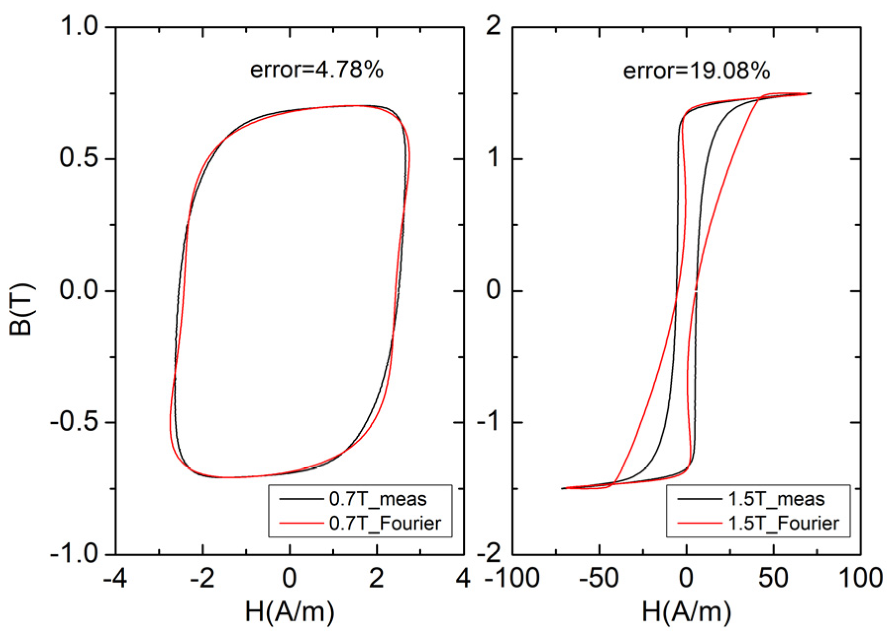
The fitting results of the hysteresis loops in the saturated region (Bm = 1.5 T) and unsaturated region (Bm = 0.7 T) obtained from the Fourier model are shown in Figure 2.
From the results in Figure 1 and Figure 2, it can be concluded that the J–A model is more suitable for fitting hysteresis loops in the saturation region, while the Fourier model is more suitable for fitting hysteresis loops in the unsaturation region. Therefore, a combination of both models can be used to fit hysteresis loop families of the same material.

4. Hybrid Hysteresis Model

4.1. Hybrid Hysteresis Model

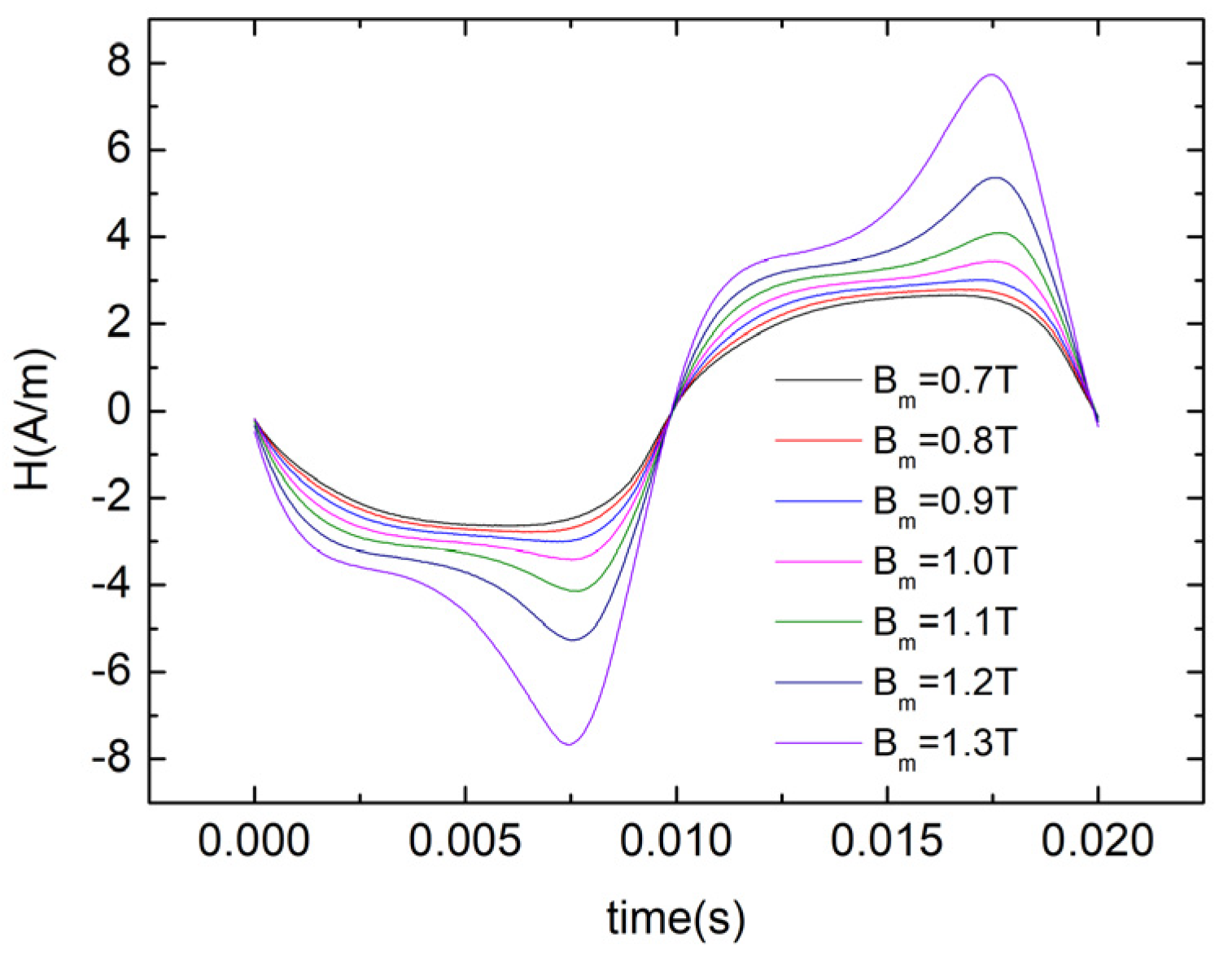
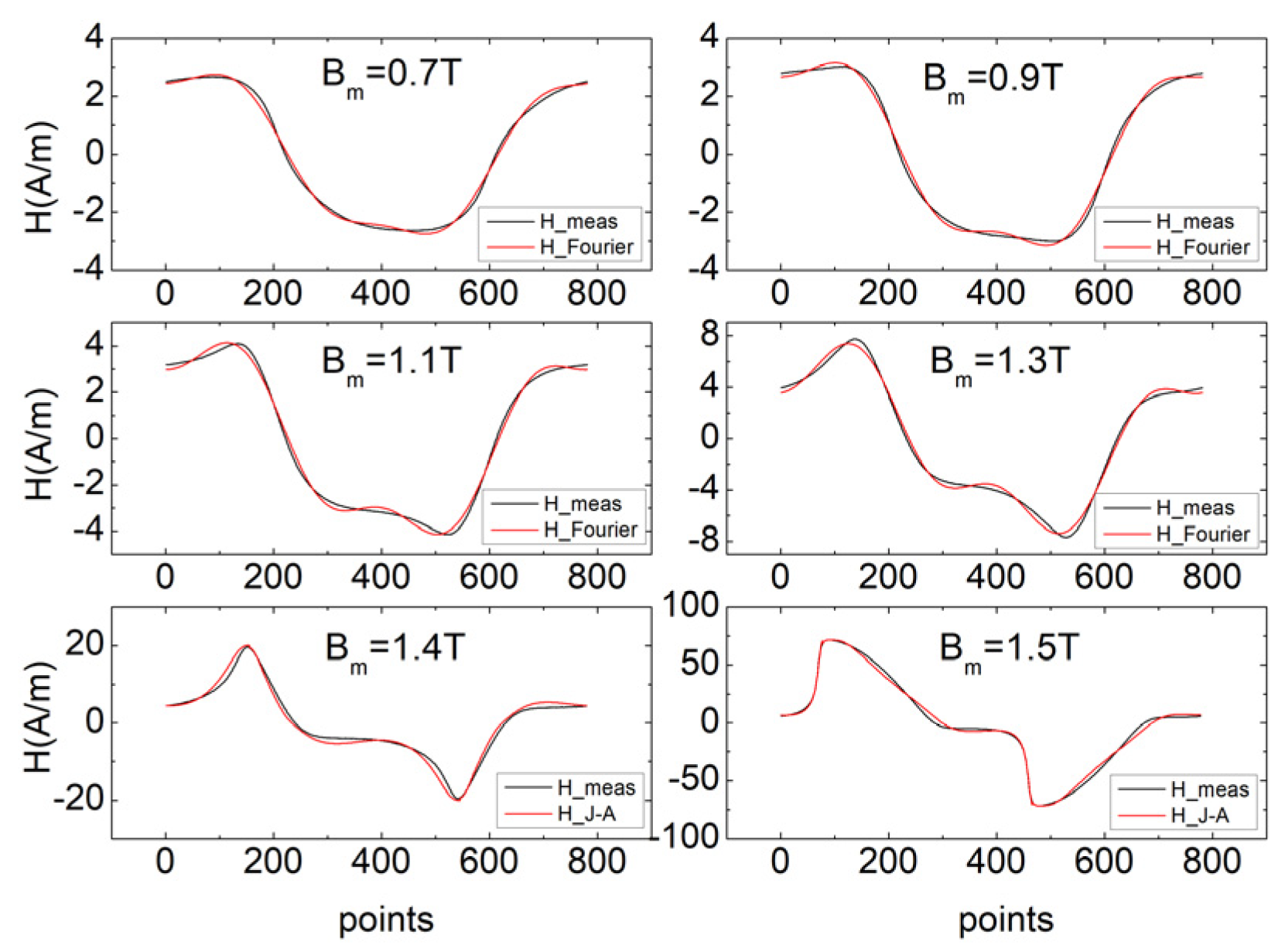
For hysteresis loops generated under sinusoidal excitation of voltage, due to the nonlinearity of the material, the magnetic field intensity H will generate waveform distortion. Therefore, the distorted waveform of H can be expressed using a Fourier series expansion. Since the distortion of H in unsaturated hysteresis loops is small, as shown in Figure 3, (especially when the saturation level is lower), fewer terms of the Fourier expansion can be used to describe it. From Figure 3, we can see that the waveform distortion of H from the measurements is increasing with the increase in B for the amorphous soft magnetic materials.
However, when it enters the saturation region, it is difficult to describe H with Fourier expansion; even though it can be described by increasing Fourier expansion terms theoretically, the parameters identification may be time-consuming work. Therefore, we can use the J–A model to obtain H easily and accurately on this occasion.
From Figure 1 and Figure 2 it can be observed that the shoulder shapes of the hysteresis loops of the amorphous soft magnetic material under research in this paper show significant differences in the unsaturated region (Bm = 0.7 T) and saturated region (Bm = 1.5 T). The unsaturated hysteresis loop has an evident elliptical shape at the shoulder, whereas the J–A model is based on the anhysteretic magnetization curve, i.e., the Langevin function with an S-like shape, which can accurately describe the shape of the saturation loops through a similar translation operation. Therefore, the elliptical character may be difficult to describe by the J–A model in unsaturated hysteresis loops. As previously mentioned, the H waveform distortion is small at this time, and the Fourier model is more suitable to be used for its description. Thus, the combination of both models can improve the overall fitting accuracy.

4.2. Calculation Time of Hybrid Hysteresis Model

Since the Fourier model has a simple functional form and does not require solving differential equations, the parameter fitting computational effort is smaller compared to the J–A model. Therefore, this paper proposes to use a hybrid model composed of the dynamic inverse J–A model and the Fourier hysteresis model to jointly fit the hysteresis loop families at different magnetic induction intensities. Experimental results show that the hybrid hysteresis model has higher fitting accuracy compared to a single hysteresis model, and it effectively reduces the computation time. Using the particle swarm optimization algorithm for parameter identification of two single hysteresis models, the computation time when the iterative number is set to 500 and 1000, respectively, was compared. The computation time of parameter identification for the fitting of a single hysteresis loop is shown in Table 1.

4.3. Critical Point of Hybrid Hysteresis Model

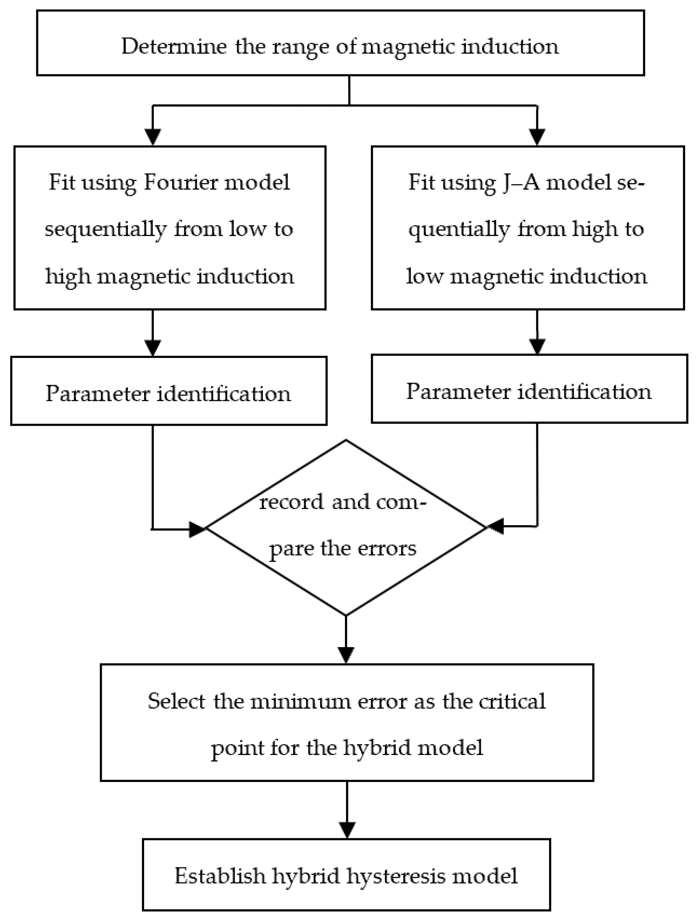
For the hybrid hysteresis model proposed in this paper, it is necessary to determine the critical point of the model. Combining theory and experimental data, it can be easily observed that when fitting using the Fourier hysteresis model in ascending order of Bm, the fitting error gradually increases, while when fitting using the J–A model in descending order of Bm, the fitting error gradually increases. The point with the smallest error is chosen as the critical point between the two models, as shown in Figure 4. The flowchart of the hybrid hysteresis model critical point testing program is shown in Figure 5.

5. Experimental Results

5.1. Testing and Fitting Results of Hysteresis Loop Families

The experimental sample studied in this paper was an amorphous soft magnetic material with a grade of 1K101. The material composition was Fe78Si9B13. It is a new type of soft magnetic material. Compared with traditional crystalline soft magnetic materials, such as oriented silicon steel and non-oriented silicon steel, it has a special microstructure without grains, which determines that it has excellent comprehensive AC soft magnetic properties such as high resistivity, high permeability, low coercivity, and low iron loss, and is an ideal soft magnetic material. The performance parameters of the experimental materials are shown in Table 2.
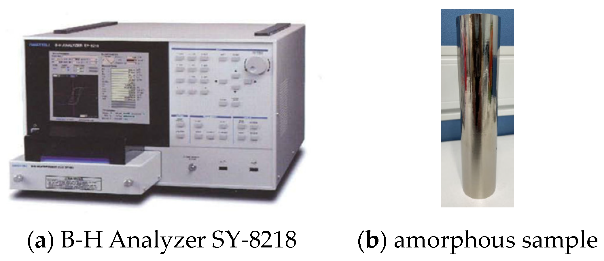
The toroidal method was adopted as the measurement method of the magnetic properties of the material, and the testing standard met the requirements of IEC international magnetic performance testing [25]. The measurement instrument and the sample are shown in Figure 6.
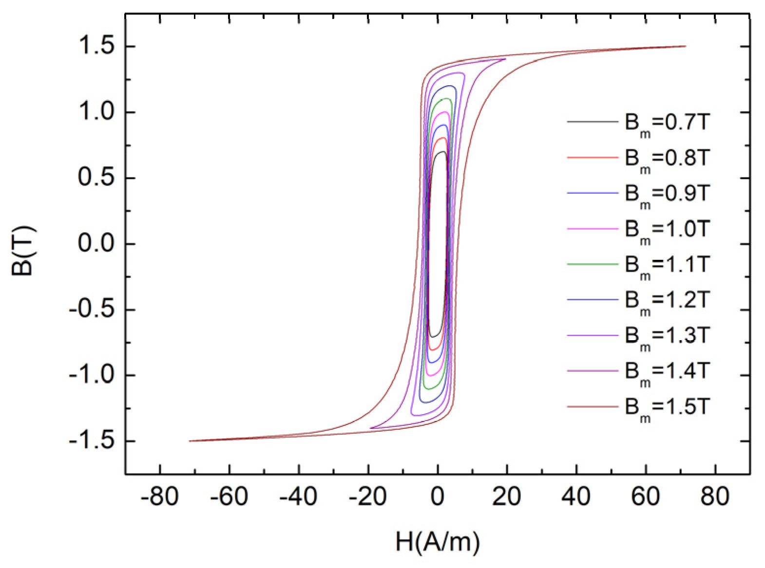
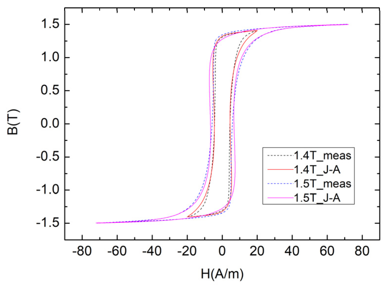
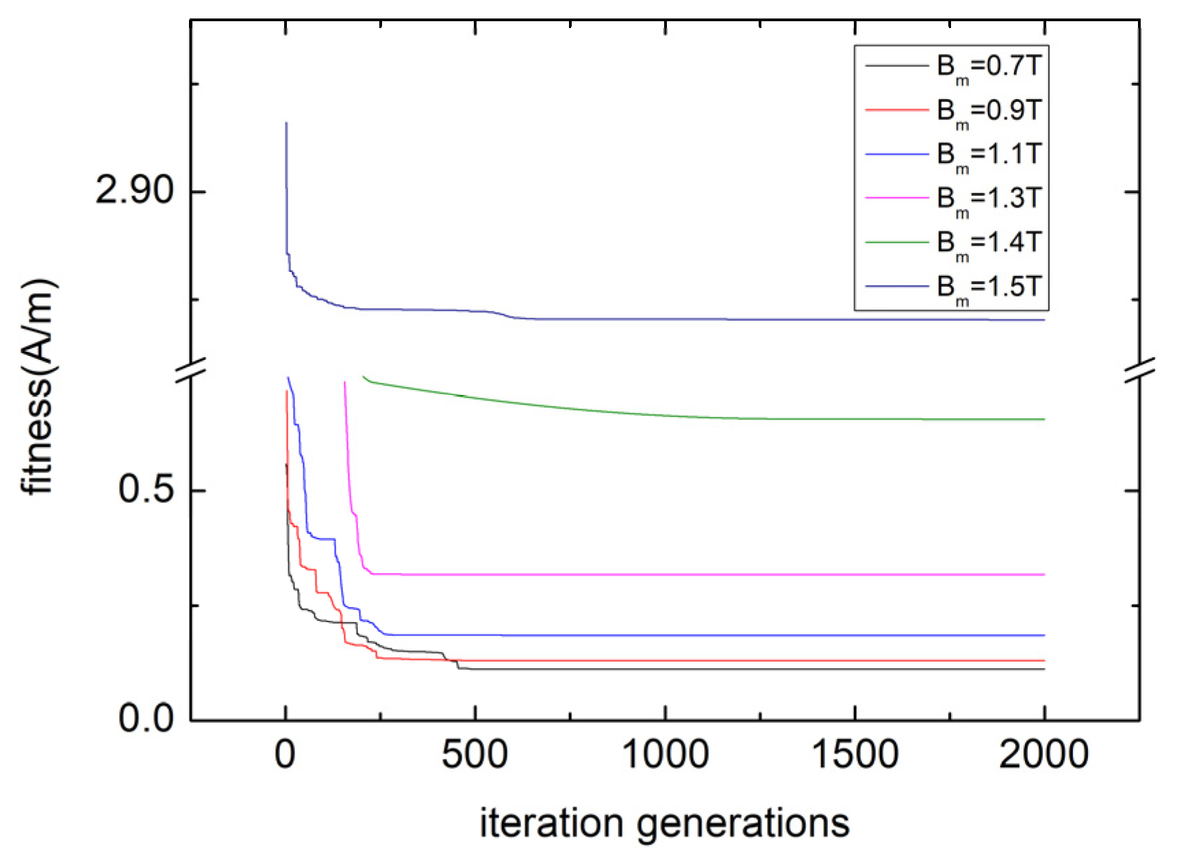
The hysteresis loops of the material were measured in the range of Bm = 0.7–1.5 T, and the measurement frequency was 50 Hz, as shown in Figure 7. Six hysteresis loops were selected for fitting using the proposed hybrid hysteresis model. According to the aforementioned critical point for the hybrid hysteresis models, the Fourier hysteresis model was used for Bm = 0.7 T, 0.9 T, 1.1 T, and 1.3 T, and the dynamic inverse J–A model was used for Bm = 1.4 T and 1.5 T. The fitting results are shown in Figure 8 and Figure 9. The waveforms of H from the hybrid models and measurements are shown in Figure 10. The hysteresis loops for any Bm value were calculated using interpolation. Both models had four parameters that needed to be fitted. The Fourier model had the parameters μ1, μ3, θ1, and θ3 to be fitted, and the J–A model had the parameters a, α, k, and c to be fitted. The parameter Ms of the J–A model was 1.24 × 10⁶. The parameter identification results are shown in Table 3 and Table 4. The fitness error was calculated using the method in Equation (19) as follows:
f i t n e s s = i = 1 N ( H m e a s ( i ) H c a l ( i ) ) 2 N .
The change of the fitness of the hybrid hysteresis model during the PSO is shown in Figure 11.
Figure 8 shows that at low magnetic induction intensities, when fitting the hysteresis loop using the Fourier hysteresis model, the fitting error gradually increased as the magnetic induction intensity increased, which is consistent with theoretical expectations.
When Bm increased to 1.4 T, it was close to the material’s saturation magnetic induction intensity, and it was more appropriate to use the J–A model for fitting, see Figure 9.
It should be noted that the dynamic inverse J–A model also contains two dynamic parameters ke and ka, which can be calculated by (3) and (4). For the given sample, the values were ke = 1.014 × 10⁻⁷ and ka = 0.3135.

5.2. Calculation Results of Losses

For comparison purposes, the proposed hybrid hysteresis model, the Bertotti model, and the single J–A and the single Fourier hysteresis models were applied to calculate losses of the testing sample. The results are shown in Table 5, where it can be seen that the overall error of the proposed hybrid hysteresis model was relatively low, with only a slightly higher error at 1.4 T. This is because this point is close to the critical point of the hybrid model and has a relative larger fitting error, as shown in Figure 4. Further improvement is needed for the hysteresis model at this point, which is a planned research topic for the next stage. Overall, the proposed hybrid hysteresis model method has a higher accuracy for loss calculation compared to the Bertotti model.

6. Conclusions

The present study proposes a hybrid hysteresis model that combines the dynamic inverse J–A model and the Fourier hysteresis model to fit the hysteresis loops of a certain amorphous soft material. Specifically, the dynamic inverse J–A model is used near the saturation region, while the Fourier hysteresis model is used in the unsaturation region. Material losses are calculated based on the hybrid hysteresis model, and the losses are also calculated using the Bertotti empirical formula model and the single J–A and the single Fourier hysteresis models for comparison. The results demonstrate that the proposed hybrid hysteresis model provides higher accuracy in loss calculation compared to the traditional Bertotti empirical formula model and the single J–A and the single Fourier hysteresis models.

Author Contributions

Conceptualization, X.F.; Writing—original draft, X.F.; Supervision, S.Y., Z.C., X.X. and Z.R. All authors have read and agreed to the published version of the manuscript.

Funding

This work was supported by the National Natural Science Foundation of China (52277019), and the Institute of Electrical Engineering, CAS (E155620101).

Data Availability Statement

The data presented in this study are available on request from the corresponding author. The data are not publicly available due to privacy.

Conflicts of Interest

The authors declare no conflict of interest.

Appendix A

Appendix A.1. Derivation of Static J–A Model Equation

By simplifying both sides of (9), we can obtain
d M i r r d H e = M a n M k δ ( 1 c ) .
Substitute (7) into (5) as follows:
M = M i r r + c ( M a n M i r r ) .
Subtract Man at both sides of (A2) as follows:
M M a n = ( 1 c ) ( M i r r M a n ) .
Substitute (A3) into (A1) as follows:
d M i r r d H e = M a n M i r r k δ .
Differentiate both sides of (5) with respect to He as follows:
d M d H e = d M i r r d H e + d M r e v d H e = d M i r r d H e + c ( d M a n d H e d M i r r d H e ) ,
and
d M d H = d M d H e d H e H = d M d H e ( 1 + α d M d H ) .
Substituting (A5) into (A6), we can obtain (10), which is consistent with reference [21].
The derivation of the static inverse J–A model requires differentiating both sides of (5) with respect to Be:
d M d B e = d M i r r d B e + d M r e v d B e = d M i r r d B e + c ( d M a n d B e d M i r r d B e ) .
and
B = μ 0 ( H + M ) .
By combining (13), (6), and (A8) as follows:
B e = B + μ 0 α M μ 0 M .
By differentiating both sides of (A9) with respect to B:
d B e d B = 1 + ( μ 0 α μ 0 ) d M d B ,
d M d B = d M d B e d B e d B .
By substituting (A7) and (A10) into (A11) and simplifying, we obtain the static inverse J–A model, as expressed in (11), which is consistent with reference [21].

Appendix A.2. Derivation of Dynamic J–A Model Equation

Simplifying (14) as follows:
M a n = M + k δ ( 1 c ) d M i r r d H e + k e d B d t d M d H e + k a d B d t 1 / 2 d M d H e .
From (A2):
M i r r = M c M a n 1 c .
Substituting (A13) into (A12), we have
d M d H e = M a n M + k δ c d M a n d H e k δ + P d .
since
d M d B = d M d B e d B e d B .
Substituting (A10) into (A15), we get
d M d B e = d M d B 1 μ 0 ( 1 α ) d M d B .
Taking the reciprocal of both sides of (A16)
1 d M d B e = 1 d M d B μ 0 ( 1 α ) .
since:
d M d H e = μ 0 d M d B e = μ 0 d M d B 1 μ 0 ( 1 α ) d M d B
By substituting (A18) into (A14) and simplifying, we obtain the dynamic inverse J–A model, as expressed in (15).

References

  1. Liu, R.; Gu, C.; Sun, J.; Shu, F.; Tang, B. Analytical Inverse Preisach Model and Its Comparison with Inverse Jiles-Atherton Model in Terms of Accuracy and Computational Speed. IEEE Trans. Magn. 2023, 59, 7300605. [Google Scholar] [CrossRef]
  2. Li, Y.; Zou, J.; Li, Y.; Zhu, J. Prediction of Core Loss in Transformer Laminated Core under DC Bias Based on Generalized Preisach Model. IEEE Trans. Magn. 2023, 60, 8400405. [Google Scholar] [CrossRef]
  3. Steinmetz, C. On the law of hysteresis (originally published in 1892). Proc. IEEE 1984, 72, 197–221. [Google Scholar] [CrossRef]
  4. Reinert, J.; Brockmeyer, A.; De Doncker, R. Calculation of losses in ferro and ferrimagnetic materials based on the modified Steinmetz equation. IEEE Trans. Ind. Appl. 2001, 37, 1055–1061. [Google Scholar] [CrossRef]
  5. Bertotti, G. Physical interpretation of eddy current losses in ferromagnetic materials. I. theoretical considerations. J. Appl. Phys. 1985, 57, 2110–2117. [Google Scholar] [CrossRef]
  6. Bertotti, G. Physical interpretation of eddy current losses in ferromagnetic materials. II. analysis of experimental results. J. Appl. Phys. 1985, 57, 2118–2126. [Google Scholar] [CrossRef]
  7. Bertotti, G.; Di Schino, G.; Milone, A.F.; Fiorillo, F. On the effect of grain size on magnetic losses of 3% non-oriented SiFe. J. Phys. Colloq. 1985, 46, 385. [Google Scholar] [CrossRef]
  8. Fiorillo, F.; Novikov, A. An improved approach to power losses in magnetic laminations under nonsinusoidal induction waveform. IEEE Trans. Magn 1990, 26, 2904–2910. [Google Scholar] [CrossRef]
  9. Jordan, H. Die ferromagnetischen konstanten für schwache wechselfelder. Elektr. Nachrichtentechnik 1924, 1, 8. [Google Scholar]
  10. Preisach, F. Über die magnetische Nachwirkung. Z. Phys. 1935, 94, 277–302. [Google Scholar] [CrossRef]
  11. Mayergoyz, I.D. Mathematical Models of Hysteresis and their Applications, 2nd ed.; Academic Press: New York, NY, USA, 2003; ISBN 9780124808735. [Google Scholar]
  12. Jiles, D.; Atherton, D. Theory of ferromagnetic hysteresis. J. Magn. Magn. Mater. 1986, 61, 48–60. [Google Scholar] [CrossRef]
  13. Jiles, D.C.; Thoelke, J.B.; Devine, M.K. Numerical Determination of Hysteresis Parameters for the Modeling of Magnetic Properties using the Theory of Ferromagnetic Hysteresis. IEEE Trans. Magn. 1992, 28, 27–35. [Google Scholar] [CrossRef]
  14. Jiles, D.C. Frequency dependence of hysteresis curves in conducting magnetic materials. J. Appl. Phys. 1994, 76, 5849–5855. [Google Scholar] [CrossRef]
  15. Rosenbaum, S.; Ruderman, M.; Strohla, T.; Bertram, T. Use of Jiles–Atherton and Preisach hysteresis models for inverse feedforward control. IEEE Trans. Magn. 2010, 46, 3984–3989. [Google Scholar] [CrossRef]
  16. Leite, J.V.; Benabou, A.; Sadowski, N. Accurate minor loops calculation with a modified Jiles-Atherton hysteresis model. COMPEL-Int. J. Comput. Math. Electr. Electron. Eng. 2009, 28, 741–749. [Google Scholar] [CrossRef]
  17. Wei, Y.; Yang, X.; Chen, Y.; Zheng, H.; Su, L. Prediction of Magnetic Losses in Giant Magnetostrictive Materials Under Different Sinusoidal Excitation Magnetic Fields. IEEE Trans. Magn. 2022, 58, 7300909. [Google Scholar] [CrossRef]
  18. Hamimid, M.; Mimoune, S.M.; Feliachi, M. Minor hysteresis loops model based on exponential parameters scaling of the modified Jiles–Atherton model. Phys. B Condens. Matter 2012, 407, 2438–2441. [Google Scholar] [CrossRef]
  19. Mörée, G.; Leijon, M. Review of hysteresis models for magnetic materials. Energies 2023, 16, 3980. [Google Scholar] [CrossRef]
  20. Krings, A.; Soulard, J. Overview and Comparison of Iron Loss Models for Electrical Machines. J. Electr. Eng. 2010, 10, 162–169. [Google Scholar]
  21. Schutte, J.F.; Groenwold, A.A. A Study of Global Optimization Using Particle Swarms. J. Glob. Optim. 2005, 31, 93–108. [Google Scholar] [CrossRef]
  22. Sadowski, N.; Batistela, N.; Bastos, J.; Lajoie-Mazenc, M. An inverse Jiles-Atherton model to take into account hysteresis in time-stepping finite-element calculations. IEEE Trans. Magn. 2002, 38, 797–800. [Google Scholar] [CrossRef]
  23. Chwastek, K. Modeling of dynamic hysteresis loops using the Jiles-Atherton approach. Math. Comput. Model. Dyn. Syst. 2009, 15, 95–105. [Google Scholar] [CrossRef]
  24. Liu, Z. Study on the Mathematical Model of Hysteresis Loop for Ferromagnetic Materials; Guangxi University: Nanning, China, 2006. [Google Scholar]
  25. IEC 60404-6:2018; Methods of Measurement of the Magnetic Properties of Magnetically Soft Metallic and Powder Materials at Frequencies in the Range 20 Hz to 100 kHz by the Use of Ring Specimens. 2018. Available online: https://webstore.iec.ch/publication/27825 (accessed on 13 April 2024).
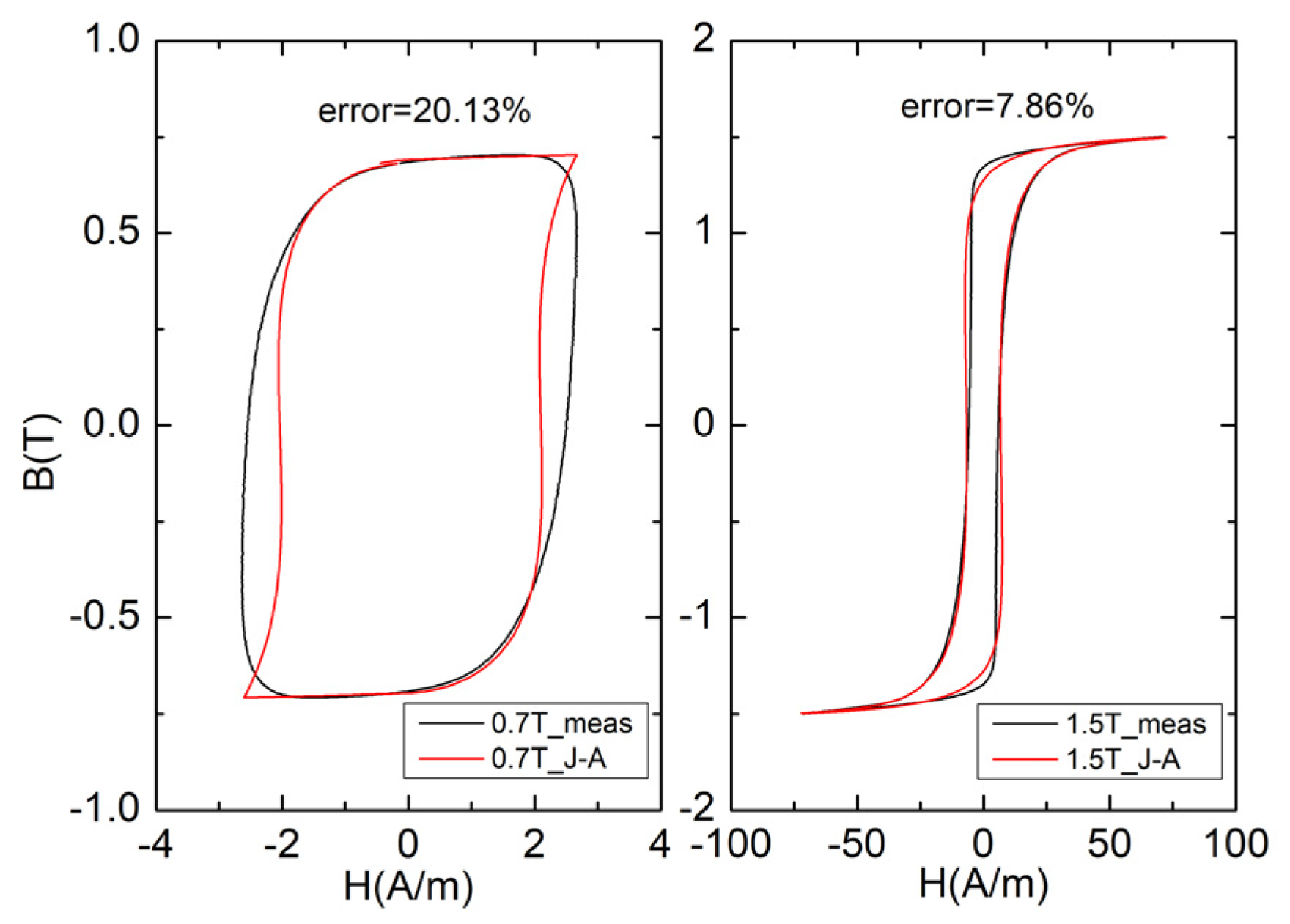
Figure 1. Fitting results of J–A model at different magnetic inductions.
Energies 17 02326 g001
Figure 2. Fitting results of Fourier hysteresis model at different magnetic inductions.
Energies 17 02326 g002
Figure 3. Waveform of H at different B.
Energies 17 02326 g003
Figure 4. The method for determining critical points of hybrid hysteresis model.
Energies 17 02326 g004
Figure 5. Flowchart for determining critical points of hybrid hysteresis models.For the material studied in this paper, the critical point for the hybrid hysteresis model is Bm = 1.35 T. When Bm > 1.35 T, the J–A model is used, and when Bm ≤ 1.35 T, the Fourier hysteresis model is used.
Energies 17 02326 g005
Figure 6. Measurement instrument (a), and sample (b).
Energies 17 02326 g006
Figure 7. Testing results of hysteresis loop families.
Energies 17 02326 g007
Figure 8. Fitting results of Fourier model for hysteresis loops.
Energies 17 02326 g008
Figure 9. Fitting results of J–A model for hysteresis loops.
Energies 17 02326 g009
Figure 10. Waveforms of H from hybrid hysteresis models and measurements.
Energies 17 02326 g010
Figure 11. Change of fitness of hybrid hysteresis model during PSO.
Energies 17 02326 g011
Table 1. Comparison of calculation times of parameter identification.
Model500 Iterations1000 IterationsComputer Configuration
J–A212.80 s423.44 s8 GB
Fourier13.38 s23.80
Table 2. Performance parameters of experimental materials.
Density
(g/cm3)
Resistivity
(μΩ·cm)
Crystallization Temperature
(T)
Saturated Magnetic Flux Density
(T)
7.181355281.56
Table 3. Results of Fourier hysteresis model parameter fitting.
Bmμ1μ3θ1θ3
0.7 T0.24−1.611.291.15
0.9 T0.39−2.21−5.050.88
1.1 T0.43−1.84−5.04−5.35
1.3 T0.21−0.641.04−5.08
Table 4. Results of J–A hysteresis model parameter fitting.
Bm (T)Ms (A/m)a (A/m)α (A/m)K (A/m)c
1.41.24 × 1061.859.88 × 10−53.740.56
1.51.24 × 10631.33 × 10−50.180.78
Table 5. Loss results by calculation and measurement.
Bm (T)Measure
(W/kg)
Hybrid Model
(W/kg)
Bertotti
(W/kg)
Error of Hybrid
Model
Error of Bertotti
0.70.044220.044290.043150.16%−2.42%
0.90.064430.06450.063090.11%−2.08%
1.10.094280.09450.09170.23%−2.74%
1.30.15150.15200.14960.33%−1.27%
1.40.20120.19500.2082−3.11%3.50%
1.50.31410.30940.3087−1.50%−1.72%
Bm (T)J–A
(W/kg)
Fourier
(W/kg)
Error of
J–A
Error of
Fourier
0.70.039940.04429−9.67%0.16%
0.90.057010.0645−11.5%0.11%
1.10.082520.0945−12.5%0.23%
1.30.12640.1520−16.5%0.33%
1.40.19500.2075−3.11%3.13%
1.50.30940.4247−1.50%35.2%
Disclaimer/Publisher’s Note: The statements, opinions and data contained in all publications are solely those of the individual author(s) and contributor(s) and not of MDPI and/or the editor(s). MDPI and/or the editor(s) disclaim responsibility for any injury to people or property resulting from any ideas, methods, instructions or products referred to in the content.