Fast Detection of the Single Point Leakage in Branched Shale Gas Gathering and Transportation Pipeline Network with Condensate Water

Abstract

The node pressure and flow rate along the shale gas flow process are analyzed according to the characteristics of the shale gas flow pipe network, and the non-leaking and leaking processes of the shale gas flow pipe network are modeled separately. The changes in pressure over time along each pipe segment in the network provide new ideas for identifying leaking pipe sections. This paper uses the logarithmic value of pressure as the basis for judging whether the flow pipe network is leaking or not, according to the process of varying flow parameters resulting in the regularity of leakage. A graph of the change in pressure of the pipe section after the leak compared to the pressure of the non-leaking section of pipe over time can be plotted, accurately identifying the specific section of pipe with the leak. The accuracy of this novel method is verified by the leakage section and statistical data of the shale gas pipeline network in situ used in this paper.

1. Introduction

1.1. Background

Rapid identification of leakage accidents in shale gas gathering and transportation pipeline networks is crucial in preventing serious consequences. Most of the research on pipeline leakage is limited to single-point or multi-point leakage identification of single pipeline, where there are relatively few studies on leakage identification of pipeline networks [1]. Existing studies have conducted a lot of research in the fields of the leak acoustic wave method [2], negative pressure wave method, optical fiber leakage identification method [3,4], pipeline real-time model method [5], most of which are applied to pipeline leakage identification and rarely applied to pipeline network leakage identification. Therefore, there is an urgent need for a rapid leak detection method to detect puncture leaks caused by corrosion or perforation in the shale gas gathering and transportation network.

1.2. Related Work

At present, there are many studies interested in the leakage problems of single-phase flow pipe networks and gas–liquid two-phase flow pipe networks, but there are very few studies on single-point leakage problems in multi-phase flow pipe networks.

1.2.1. Leak Detection and Location of Single-Phase Flow Pipe Network

In order to improve the accuracy of gas pipeline network leak location, Wu and Lee [6] proposed an improved leak location method based on AE signals and combined an improved generalized cross-correlation location method and an attenuation-based multi-layer perceptron neural network (MLPNN) location method. Kabaasha et al. [7] imported the corrected orifice plate leakage equation into the liquid pipe network formula and applied conventional and improved software to 600 random leakage distribution examples in three different pipe networks. Hongwei Li et al. [8] simulated the complex liquid pipeline network system and established an experimental platform. Based on this, a leak detection method using improved wavelet denoising and short-time Fourier transform was proposed, which can be used for real-time monitoring of pipeline network leakage. Walt et al. [9] investigated an inversion analysis technique to determine leakage in a liquid pipeline network.

1.2.2. Research on Leak Detection and Location of Multiphase Flow Pipelines

Liu et al. [10] studied a new acoustic wave-based leak detection and location method for oil and gas pipelines, and established and modified the propagation model. Rai and Kim [11] proposed a method based on multi-scale analysis, Kolmogorov–Smirnov (KS) test, and Gaussian Mixture Model (GMM) to determine the leakage of oil and gas pipelines. Oyedeko and Balogun [12] studied the transient flow analysis of the fluid in the pipeline to develop a control system to detect leaks, locate leaks, and determine their flow. Lukonge et al. [13] summarized the techniques for identifying and extracting wave features in detail and revised the leak location formula for pipelines.

1.2.3. Research on Leak Detection and Location of Multiphase Flow Pipe Network

Sarkamaryan et al. [14] proposed a corrected inverse transient analysis (ITA) for leak detection and calibration of pipeline networks. Aida-zade [15] numerically solved the inverse problem of a pipeline network with a complex loop structure to determine the location and number of leaks. At present, there are relatively few studies on the identification of single point leaks in multiphase flow pipe networks, so it is necessary to investigate a method that will identify the leakage of the multiphase flow pipe network and reduce the safety accidents and economic losses caused by the leakage.

1.3. The Contribution of This Work

This paper mainly studies the identification of the leaking pipe section after a single- point leakage in the dendritic shale gas gathering and transportation network. First, the pressure changes after the leak of the shale gas gathering pipeline network are analyzed, and then the leaking section of the shale gas flow pipe network is preliminarily assessed. Finally, based on the rate of pressure drop, a method is proposed to quickly identify leaking pipe sections.

2. Materials and Methods

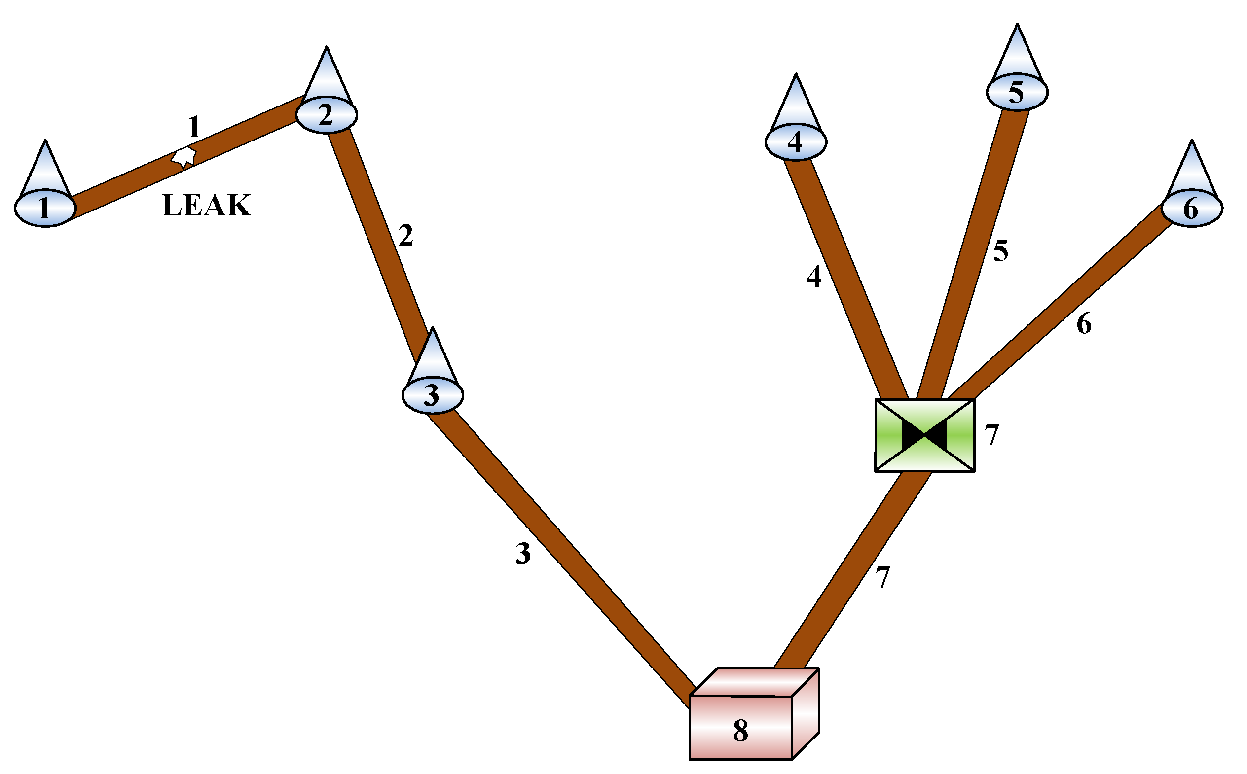
2.1. Problem Description and Model Assumptions

This paper focuses on the leakage identification problem of shale gas containing condensate water gathering and transportation network. The topological structure diagram of shale gas gathering and transportation network, and the schematic diagram of leakage points, are shown in Figure 1.

The pipe length, pipe diameter, leakage aperture, temperature, pressure, flow rate, gas–liquid ratio and other parameters of the trunk and branch lines of the shale gas gathering, and transportation network are known. Based on the calculation of the hydraulic and thermal energy of the pipe network, the changes in pressure, temperature, liquid holdup rate, and gas and liquid flow rate of the pipe network are analyzed. Based on the rate of change in these key fluid parameters, this research proposes a method for rapid leak detection.

2.2. Transient Model for Gas–Liquid Two Phase Pipe Network Flow and Single Point Leakage

The shale gas gathering and transportation network model is established by using the control equation set of one-dimensional flow in a two-phase gas–liquid pipeline network. Then, the different leakage situations of the pipeline network are simulated, where the effects of single-point leakage in different pipeline sections on the temperature, pressure, liquid holdup, and gas–liquid flow rate of the pipeline network are separately analyzed. A three-dimensional diagram of the change in the parameters of the entire pipeline network before and after the leakage is drawn to conduct in-depth research on the leakage identification of the pipeline network.

The two-fluid model [16,17] usually contains the following six equations: the mass equation, momentum equation, and energy equation of the gas and liquid phases, respectively. In this study, a two-fluid model is established based on the following three assumptions: (1) It is a one-dimensional flow; (2) there is no axial heat conduction or heat radiation along the pipe; and (3) the liquid and gas phases have the same pressure at the same cross section of the pipe. The two-fluid model is a set of quasi-linear partial differential equations, in which the main variables are P, ${\alpha }_g$, v_g, v_l, u_l and u_g, and other parameters can be calculated from the closed relationship.

The mass conservation equation is as follows:

$$\frac{\mathit{\partial }}{\mathit{\partial }t}\left({\rho }_{\mathrm{g}}{\alpha }_{\mathrm{g}}\right)+\frac{\mathit{\partial }}{\mathit{\partial }x}\left({\rho }_{\mathrm{g}}{\alpha }_{\mathrm{g}}{v}_{\mathrm{g}}\right)=\Delta {\dot{m}}_{\mathrm{gl}}$$

(1)

$$\frac{\mathit{\partial }}{\mathit{\partial }t}\left({\rho }_1{\alpha }_1\right)+\frac{\mathit{\partial }}{\mathit{\partial }x}\left({\rho }_1{\alpha }_1{v}_1\right)=\Delta {\dot{m}}_{\lg }$$

(2)

where the subscripts l and g represent the liquid and gas phases, respectively; t is for time, s; x is the distance, m; $\rho$ is the density, kg/m³; v is the velocity, m/s, ${\alpha }_g$ is the vapor void ratio; ${\alpha }_1$ is the liquid void fraction; $\Delta {\dot{m}}_{\mathrm{gl}}$ is the liquid mass transfer rate per unit volume, kg/(m³·s); $\Delta {\dot{m}}_{\lg }$ is the mass transfer rate of gas per unit volume, kg/(m³·s).

The momentum conservation equation is as follows:

$$\frac{\mathit{\partial }}{\mathit{\partial }t} \left({\alpha }_{\mathrm{g}}{\rho }_{\mathrm{g}}{v}_{\mathrm{g}}\right)+\frac{\mathit{\partial }}{\mathit{\partial }x}\left({\alpha }_{\mathrm{g}}{\rho }_{\mathrm{g}}{v}_{\mathrm{g}}^2\right)+{\tau }_{\mathrm{wg}}{\mathrm{S}}_{\mathrm{g}}+{\tau }_{\mathrm{i}}{S}_{\mathrm{i}}=-{\alpha }_{\mathrm{g}}{\rho }_{\mathrm{g}}g\sin \theta -{\alpha }_{\mathrm{g}}\frac{\mathit{\partial }{P}_{\mathrm{g}}}{\mathit{\partial }\mathrm{x}}+\Delta {\dot{m}}_{\mathrm{gl}}{v}_{\mathrm{i}}$$

(3)

$$\frac{\mathit{\partial }}{\mathit{\partial }t}\left({\alpha }_1{\rho }_1{v}_1\right)+\frac{\mathit{\partial }}{\mathit{\partial }x}\left({\alpha }_1{\rho }_1{v}_1^2\right)+{\tau }_{\mathrm{wl}}{S}_1-{\tau }_{\mathrm{i}}{S}_{\mathrm{i}}=-{\alpha }_1{\rho }_{1}g\sin \theta -{\alpha }_1\frac{\mathit{\partial }{P}_1}{\mathit{\partial }x}+\Delta {\dot{m}}_{\lg }{v}_{\mathrm{i}}$$

(4)

where the subscript i refers to the phase between the liquid and gas phases; P is the total pressure, Pa; S is the wall circumference in contact with the liquid or gas phase, 1/m; ${\tau }_{\mathrm{i}}$ is the shear stress between phases at the interface, Pa; ${\tau }_{\mathrm{wg}}$ and ${\tau }_{\mathrm{wl}}$ are respectively the gas phase and liquid phase shear stresses acting on the tube wall, Pa; $\theta$ is the Angle of the pipe, rad.

The energy conservation equation is as follows:

$$\begin{array}{l}\frac{\mathit{\partial }}{\mathit{\partial }t}\left\{{\rho }_{\mathrm{g}}{\alpha }_{\mathrm{g}}\left(u_{\mathrm{g}}+\frac{v_{\mathrm{g}}^2}{2}\right)\right\}+\frac{\mathit{\partial }}{\mathit{\partial }x}\left\{{\rho }_{\mathrm{g}}{\alpha }_{\mathrm{g}}{v}_{\mathrm{g}}\left(u_{\mathrm{g}}+\frac{v_{\mathrm{g}}^2}{2}\right)\right\}+q_{\mathrm{i}}{S}_{\mathrm{i}}\hfill \\ =-{\rho }_{\mathrm{g}}{\alpha }_{\mathrm{g}}{v}_{\mathrm{g}}g\sin \theta -\frac{\mathrm{a}\left(P_{\mathrm{g}}{\alpha }_{\mathrm{g}}{v}_{\mathrm{g}}\right)}{\mathit{\partial }x}+{\tau }_{\mathrm{i}}{S}_{\mathrm{i}}{v}_{\mathrm{i}}-q_{\mathrm{wg}}{S}_{\mathrm{g}}+\Delta {\dot{m}}_{\mathrm{gl}}\left(u_{\mathrm{i}}+\frac{v_{\mathrm{i}}^2}{2}\right)\hfill \end{array}$$

(5)

$$\begin{array}{l}\frac{\mathit{\partial }}{\mathit{\partial }t}\left\{{\rho }_1{\alpha }_1\left(u_1+\frac{v_1^2}{2}\right)\right\}+\frac{\mathit{\partial }}{\mathit{\partial }x}\left\{{\rho }_1{\alpha }_1{v}_1\left(u_1+\frac{v_1^2}{2}\right)\right\}-q_{\mathrm{i}}{S}_{\mathrm{i}}\\ =-{\rho }_1{\alpha }_1{v}_{1}g\sin \theta -\frac{\mathit{\partial }\left(P_1{\alpha }_1{v}_1\right)}{\mathit{\partial }x}-{\tau }_{\mathrm{i}}{S}_{\mathrm{i}}{v}_{\mathrm{i}}-q_{\mathrm{wl}}{S}_1+\Delta {\dot{m}}_{\lg }\left(u_{\mathrm{i}}+\frac{v_{\mathrm{i}}^2}{2}\right)\end{array}$$

(6)

where u is for inner energy; h is enthalpy, J/kg; $q_{\mathrm{wg}}$ and $q_{\mathrm{wl}}$ are the heat transferred from the tube wall to the liquid and gas phases, respectively, J/(m²·s); $q_{\mathrm{i}}$ is the heat transfer exchanged at the interface, J/(m²·s).

Gas leakage in pipeline transportation is a complex process. After a leak occurs, the gas flows from the pipeline to the surrounding environment. During the flow process, the real gas undergoes a sudden reduction in cross-section, resulting in a Joule Thomson effect and a decrease in gas temperature. At the same time, the pressure at the leakage hole will attenuate and transmit pressure relief waves upstream and downstream of the pipeline. The huge pressure difference inside and outside the pipeline can easily generate a jet at the leakage point [18]. Based on engineering practice, a pipeline large hole leakage model is selected [19], the leakage aperture size is set to 25 mm, and the backpressure at the leak hole is set at 1 atmosphere. The gas flow at the leakage hole is supersonic. At this time, the pressure, temperature, and density at various points on the same cross-section are not equal. The leakage rate of natural gas is as follows:

$$Q=C_d{A}_h{p}_b\sqrt{\frac{Mk}{ZR{T}_b}·{\left(\frac{2}{k+1}\right)}^{\frac{k+1}{k-1}}}$$

(7)

where C_d is the flow coefficient of the gas at the leakage point; A_h is the leakage area, m²; P_b is the pressure at the center point of the leak, Pa; M is the molecular weight of natural gas, kg/kmol; k is the Gas adiabatic index, dimensionless; Z is the Gas compressibility factor; T_b is the temperature at the center point of the leak, K; R is the gas constant, usually taken as 8.314 kJ/(kmol k) for natural gas.

The flash method is used to calculate the physical properties of the fluid and the fluid flow inside the pipeline. Based on this, the fluid flowing process model is established, where the mutual influence of condensate and pressure is clarified.

2.3. Verification Method for the Effectiveness of Leak Detection Technology

The effectiveness of pipeline leak detection technology refers to its ability to continuously detect pipeline leaks. Currently, the most widely used and promising leak detection methods include the distributed fiber-optic method, the transient model method, and the acoustic wave method.

The distributed fiber-optic method detects leaks through the vibration and temperature changes of the soil around the leakage point. Currently, the temperature threshold method is commonly used to alert the leakage location. By using optical fibers laid along the pipeline to obtain temperature changes at various points, the difference T₀ between the temperature T and the average temperature along the pipeline is compared with the temperature threshold set by the distributed optical fiber monitoring system. If $T-T_{{ }_0}>3\mathrm{\sigma }$, the system sounds an alarm indicating that a specific point in the pipework is leaking [20]. The temperature measurement accuracy of this method is around 1 °C, the positioning error range is within 5 m and the response time is within 5 s.

The transient model method is a method that combines flow rate and pressure to determine whether a pipeline has occurred the leakage. By simulating the changes in parameters such as temperature, pressure and flow rate at the start and end points and comparing them with the parameters before the leak. If the relative error between the two exceeds a certain threshold, it can be determined that the pipeline is leaking. Based on previous experience, a leakage rate of 4% of the internal flow rate was chosen as the flow rate threshold, and an empirical value of 0.15 MPa/min for the gas transmission main line shut-off valve was chosen as the pressure drop rate threshold [21]. This method can control the leakage accuracy to about 1%.

The acoustic wave method receives and collects acoustic signals through acoustic sensors installed at both ends of the pipe. The acoustic signal is usually represented by the change in amplitude of the acoustic wave over time. After de-noising and extracting the collected wave signal, the acoustic wave amplitude without leakage is taken as the threshold value and compared with the real time acoustic signal, to determine whether leakage has occurred in the pipeline [22]. When used for gas pipeline leak detection, the minimum detectable leak is 0.01% of the transported volume. For long distance pipelines, the positioning accuracy is approximately 50 m and the response time is less than 3 min.

By comparing the above three pipeline leak detection technologies, the validity verification indexes, and threshold names of each detection technology are obtained as shown in

Table 1. Threshold value of validity verification method of leakage detection technology.

Pipeline Leak Detection Technology	Threshold Variable Name	Representative Formula	Value Position	Value Sequence
Distributed fiber optic method	Vibration amplitude, temperature	δA, δA/δt	Starting and ending points, intermediate nodes	Time series
Transient model method	change/rate of change value	δT, δT/δt	Starting and ending points,	Time series
Acoustic wave method	Pressure simulation value	δP, δP/δt	Starting and ending points, intermediate nodes	Time series

.

2.4. Identification Method for Single Point Leakage in Gas-Liquid Two-Phase Flow Pipeline Network Based on Pressure Drop Rate

The NPW (negative pressure wave) produced by the leakage propagating up and down simultaneously at the speed $a$. The produced NPW is detected by the sensors at $t$ and $t+\Delta t$ time, respectively, with pressure signals $p_u(t+\Delta t)$ and $p_d(t)$ when l₁ > l₂. According to the leakage data, the $\frac{\mathit{\partial }p}{\mathit{\partial }t}$ in the upstream and downstream are functions related to $t$, and the shapes of line A and B are very similar.

The sum of the pressure node values of pipe section i in the non-leaking pipe network is $\sum P_0\left(i\right)$, while in the leaking pipe network, it is $\sum P_t\left(i\right)$. The average value of the pressure node value of pipe section i in the non-leaking pipe network is $\overline{\sum {P_0}_{\left(i\right)} }$, while in the leaking pipe network, it is $\overline{\sum {P_t}_{\left(i\right)} }$. Therefore, when the leakage time is t, the pressure drop in pipe section i in the pipe network is:

$$Nt\left(i\right)=\frac{\overline{\sum {P_t}_{\left(i\right)} }-\overline{\sum {P_0}_{\left(i\right)} }}{\overline{\sum {P_0}_{\left(i\right)} }}$$

(8)

where i represents a certain pipe section in the pipe network; t represents the leakage time of the pipe network; N_t(i) represents the pressure change range of the pipe section i after the leakage time t. After the sum of the pressure node values of pipe section i with different leakage time t being simulated, the pressure change range N_t(i) of pipe section i is then calculated. The leakage time log(t) and N_t(i) are applied to plot the pressure variation amplitude curve of the pipe section with leaked point after leakage. Then, the change amplitude curve is shown in Figure 2.

3. Application Example of Leaking Pipe Segment Identification Method Based on Pressure Drop Rate

The non-leakage pipeline network and single-point leakage pipeline network models of gas-liquid two-phase flow are established. The selected block is a gathering and transportation network consisting of seven pipelines. The basic parameters of the network are shown in

Table 2. Parameters of the pipe network.

Pipe Segment No.	1	2	3	4	5	6	7
Diameter (mm)	160	160	225	160	160	160	325
Length (km)	1.00	1.00	0.60	1.14	1.20	1.00	1.20
Thickness (mm)	6.00	6.00	9.50	6.00	6.00	6.00	12.80

. The annual average surface temperature of this block is 273 K and the initial conditions of the pipe network are shown in

Table 3. Initial conditions of the pipe network.

Pipe Segment No.	1	2	3	4	5	6	7	8
Mass flowrate (kg/s)	1	1	1	2	2	2	0	9
Pressure (MPa)	—	—	—	—	—	—	—	0.3
Temperature (K)	305	305	295	305	305	305	295	285
Gas content ratio (-)	0.9	0.9	0.9	0.9	0.9	0.9	0.9	0.9

. The boundary conditions and initial conditions used for establishing the pipeline model are shown in the

Table 4. Boundary conditions and initial conditions.

Parameter	Equation
Initial Condition	$Q_{i,j,0}=Q_{i,j,initial},x_{i,j,0}=x_{i,j,initial},T_{i,j,0}=T_{i,j,initial},P_{i,j,0}=P_{i,j,initial}$
Entrance Boundary Conditions	$G_{i,1,k}=G_{i,in,k},T_{i,1,k}=T_{i,in,k}$
Export Boundary Conditions	$P_{CPF,k}^{out}=P_{CPF,k}^{in}$
Node Boundary Conditions	$P_{in,1,k}=P_{in,2,k}=P_{out,k},x_{out,k}=\left(\sum x_{in,k}{G}_{in,k}\right)/G_{out,k}$ $G_{out,k}=\sum G_{in,k},T_{out,k}=\left(\sum {c_p}_{,in,k}{T}_{in,k},G_{in,k}\right)/\left({c_p}_{,out,k}{G}_{out,k}\right)$

.

The transmission fluid of the pipeline network is shale gas and water. Two single point leakage models of pipe section 4 and pipe section 7 are constructed using the given initial conditions and basic parameters of the pipe network (shown in Figure 3), respectively. Both pipe section 4 and pipe section 7 leak at 500 m, where the leak hole diameter is 25 mm, and the leak time is 10 min. The one-dimensional flow control equations are used to calculate the two leakage conditions of the pipe network, giving the changes in pressure, temperature, liquid holdup, and gas-liquid flow rate of the leaking pipe section and the entire pipe network before and after the leakage.

3.1. Change Rule of Pipeline Parameters before and after Leakage

3.1.1. The Law of Pressure Change

The pressure changes in pipe section 4 and pipe section 7 before and after the leak occurred are shown in Figure 4 and Figure 5, respectively. The pressure in the pipe sections before and after the leak is reduced, and the pressure after the leak is lower than before the leak. The pressure of pipe section 4 decreases from 0.69 MPa to 0.45 MPa before the leak, and the pressure decreases from 0.65 MPa to 0.45 MPa after the leak. The pressure in pipe section 7 drops from 0.44 MPa to 0.36 MPa before the leak, and from 0.43 MPa to 0.35 MPa after the leak.

3.1.2. The Law of Temperature Change

The temperature changes in pipe section 4 and pipe section 7 before and after the leakage occurred are shown in Figure 6 and Figure 7, respectively. The temperature along the pipe network before and after the leak is reduced, and the temperature after the leak is lower than before the leak. The temperature of pipe section 4 dropped from 31.8 °C to 26.3 °C before the leak and from 31.7 °C to 26.2 °C after the leak. The temperature of pipe section 7 dropped from 26.7 °C to 23.9 °C before the leak and from 26.3 °C to 23.1 °C after the leak.

3.1.3. Change Law of Liquid Holdup

The changes in liquid holdup of the pipe sections before and after the leak in pipe section 4 and pipe section 7 are shown in Figure 8 and Figure 9, respectively. The liquid holdup of the pipe section before and after the leak shows a general downward trend, and the liquid holdup after the leak is lower than before the leak.

3.1.4. The Law of Gas Flow Rate Change

The changes in gas flow velocity in the pipe sections before and after the leak in pipe section 4 and pipe section 7 are shown in Figure 10 and Figure 11, respectively. The gas flow rate of the pipe network before and after the leak shows an overall upward trend. The gas velocity increases from 23.5 m/s to 36.2 m/s before the leak in pipe section 4 and increases from 25.4 m/s to 29.6 m/s after the leak, with a sudden change at the 500 m leak. The gas velocity increases from 26.7 m/s to 32.8 m/s before the leak in pipe section 7 and increases from 27.5 m/s to 32.1 m/s after the leak, which also shows a sudden change at the 500 m leak.

3.1.5. The Law of Change in Liquid Flow Rate

The changes in liquid flow rate in the pipe sections before and after the leak in pipe section 4 and pipe section 7 are shown in Figure 12 and Figure 13 respectively. The liquid flow rate before and after the leak shows an overall downward trend, and the liquid flow rate after the leak is lower than before the leak.

3.2. Changes in the Parameters of the Entire Pipeline Network before and after the Leak

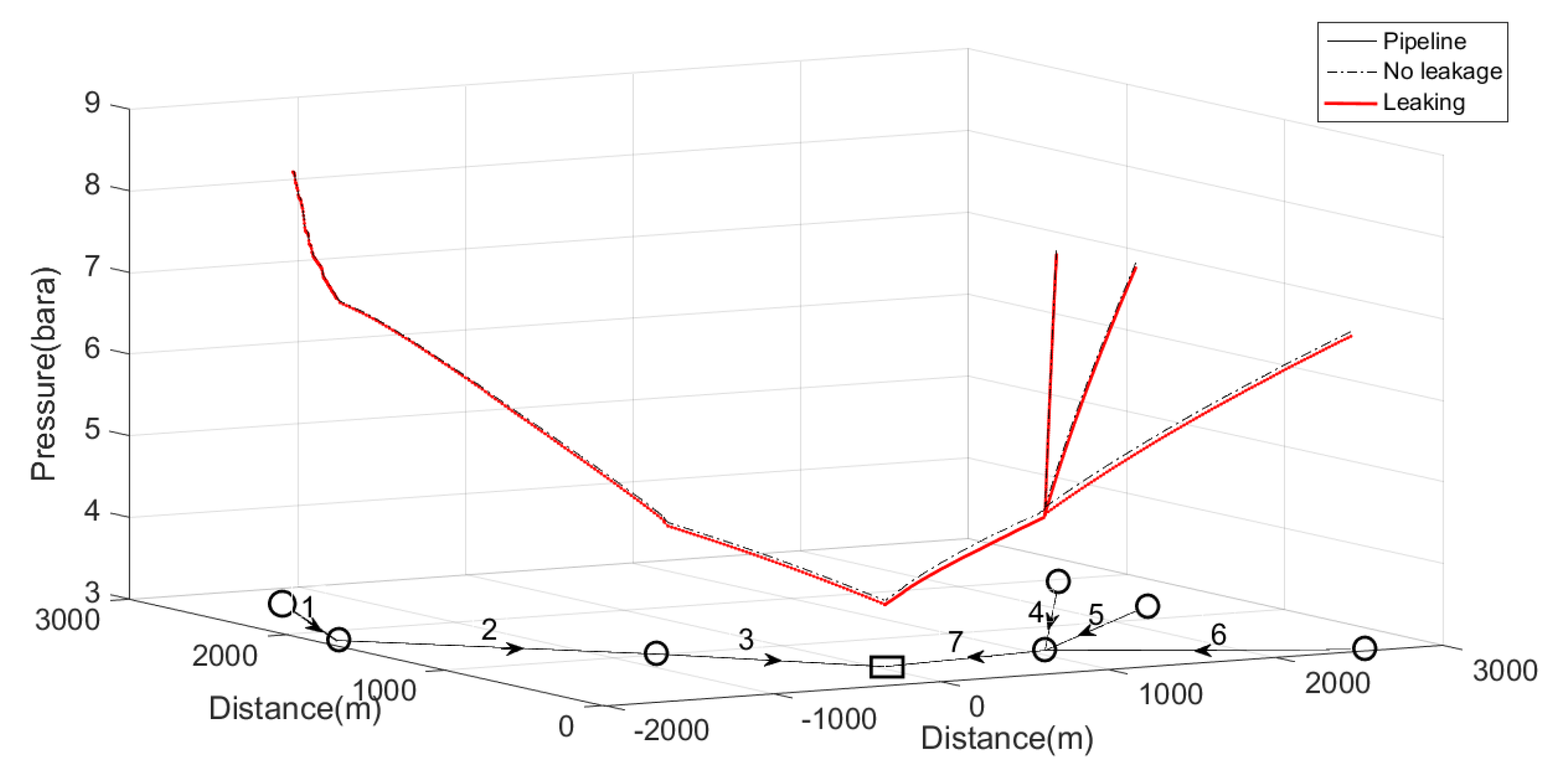
3.2.1. The Law of Pressure Changes along the Pipeline

The changes in the network pressure before and after the leakage of pipe section 4 and pipe section 7 are shown in Figure 14 and Figure 15. The pressure of all pipe sections before and after the leakage decreased, and the pressure after the leak was lower than that before the leak, especially the pressure drop of the leaking pipe section is greater than that of the other non-leaking pipe sections. Numbers 1–7 represent the numbering of each pipe segment in the pipeline network. Same as Figure 15, Figure 16, Figure 17, Figure 18, Figure 19, Figure 20, Figure 21, Figure 22 and Figure 23.

Figure 14. Changes in pressure in pipeline network before and after the leakage happened in pipe section 4.

Figure 14. Changes in pressure in pipeline network before and after the leakage happened in pipe section 4.

Figure 15. Changes in pressure in pipeline network before and after the leakage happened in pipe section 7.

Figure 15. Changes in pressure in pipeline network before and after the leakage happened in pipe section 7.

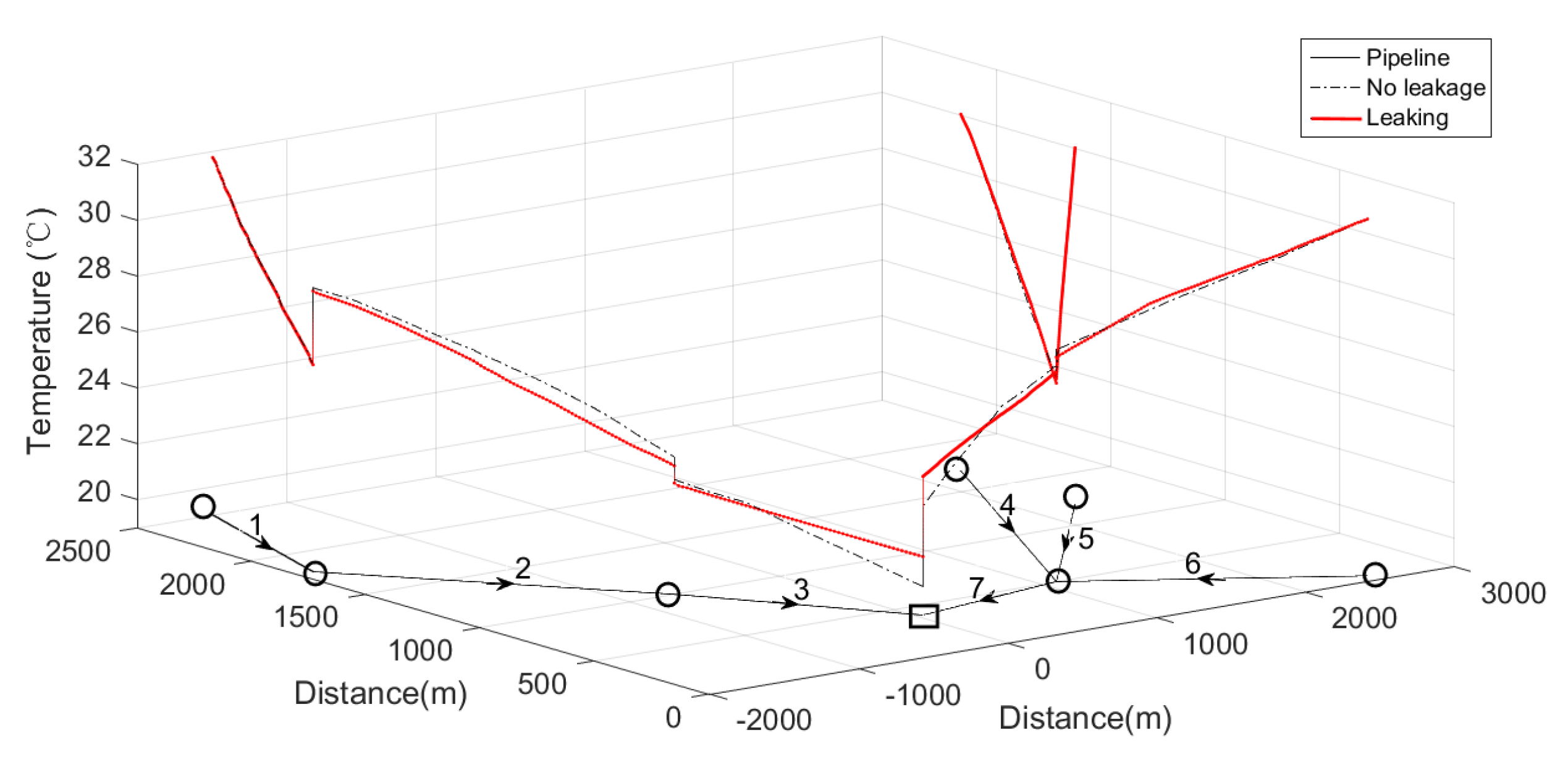
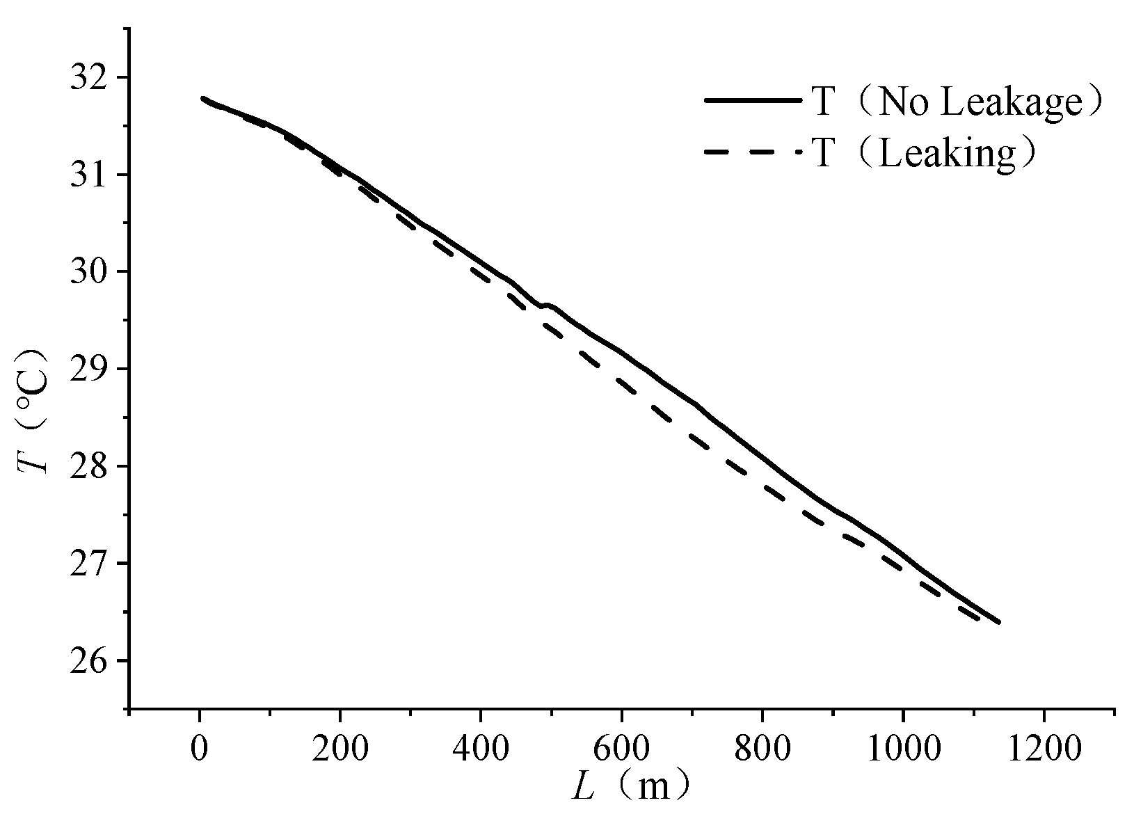
3.2.2. The Law of Temperature Changes along the Pipeline

The temperature changes in the pipe network before and after the leak in pipe section 4 and pipe section 7 are shown in Figure 16 and Figure 17. The temperature of all pipe sections decreased before and after the leak, and the temperature decrease trend after the leak is the same as before the leak.

Figure 16. Change in temperature in pipeline network before and after leakage happened in pipe section 4.

Figure 16. Change in temperature in pipeline network before and after leakage happened in pipe section 4.

Figure 17. Change in temperature in the pipeline network before and after the leakage happened in pipe section 7.

Figure 17. Change in temperature in the pipeline network before and after the leakage happened in pipe section 7.

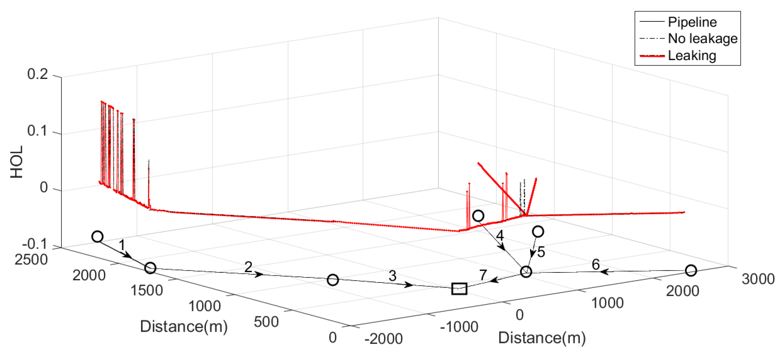
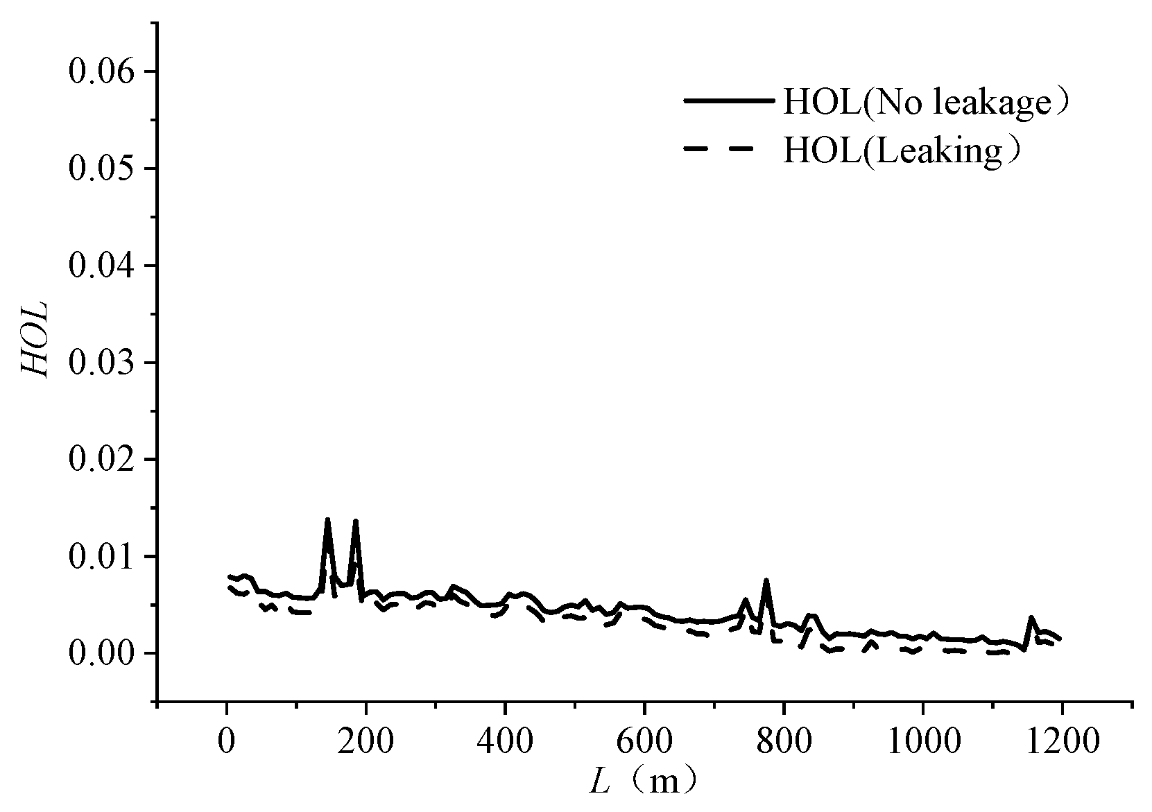
3.2.3. The Law of Liquid Holdup Changes along the Pipeline

The change rule of the liquid holdup of the pipe network before and after the leak of pipe section 4 and pipe section 7 is shown in Figure 18 and Figure 19. The liquid holdup rate before and after the leak showed a downward trend, and the liquid holdup rate after the leak is slightly lower than before the leak.

Figure 18. Changes in liquid holdup in pipeline network before and after the leakage happened in pipe section 4.

Figure 18. Changes in liquid holdup in pipeline network before and after the leakage happened in pipe section 4.

Figure 19. Changes in liquid holdup in pipeline network before and after the leakage happened in pipe section 7.

Figure 19. Changes in liquid holdup in pipeline network before and after the leakage happened in pipe section 7.

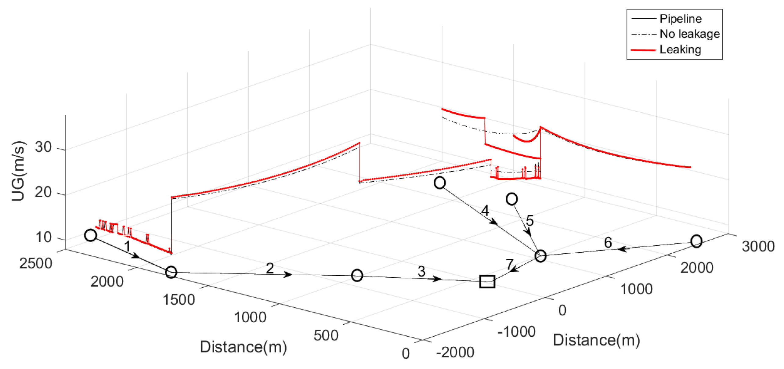
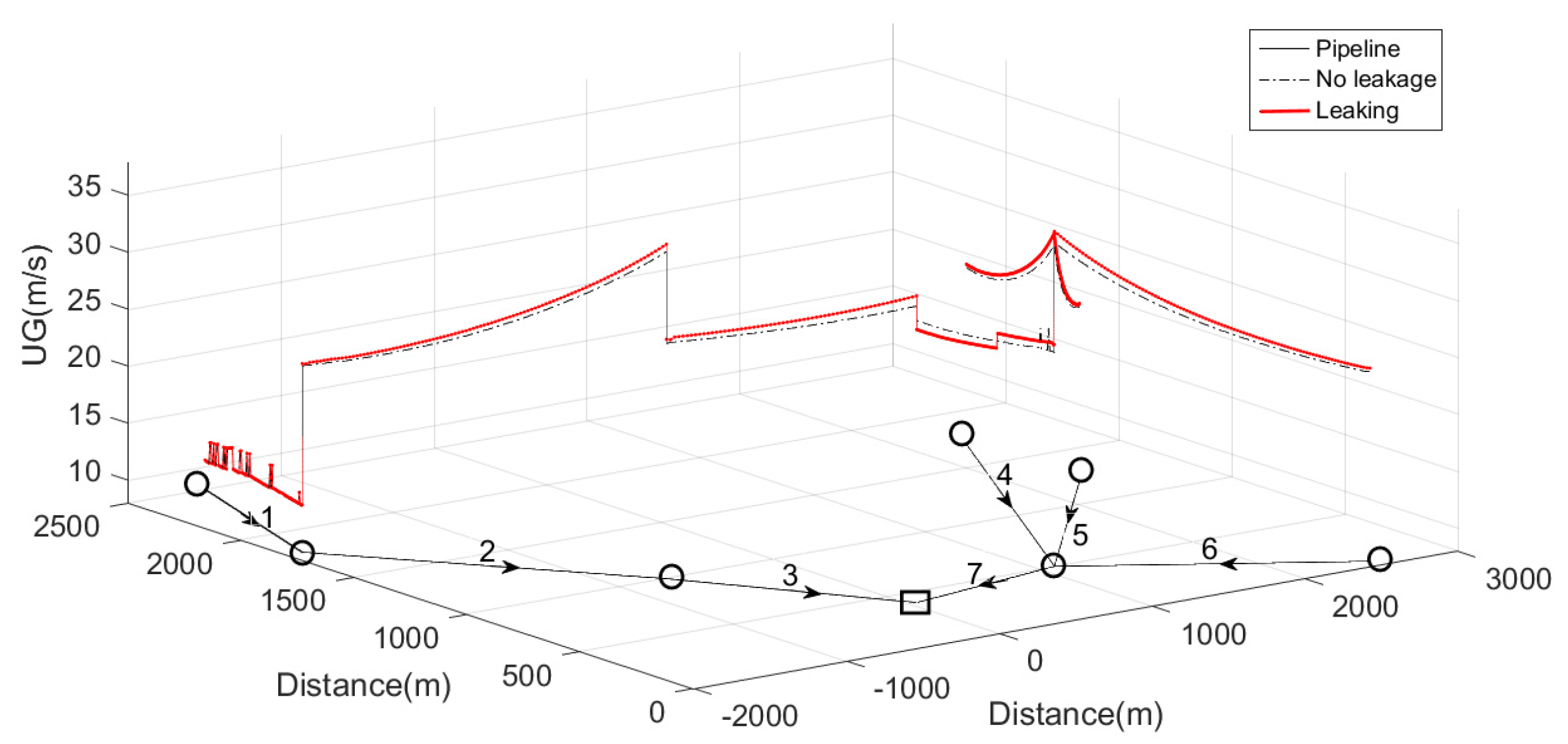
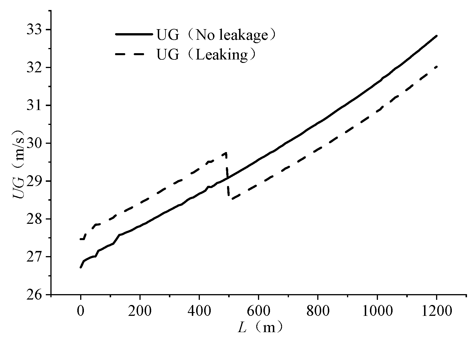
3.2.4. The Gas Flow Rate Changes along the Pipeline

The change rule of the gas flow rate of the pipe network before and after the leakage of pipe section 4 and pipe section 7 is shown in Figure 20 and Figure 21. The gas flow rate before and after the leak showed an upward trend. The gas flow rate at the leak point of the leaking pipe section shows a sudden change. The gas flow rate before the leak is higher than without the leak and the gas flow rate after the leak is lower than without the leak.

Figure 20. Changes in gas flow rate in pipeline network before and after the leakage happened in pipe section 4.

Figure 20. Changes in gas flow rate in pipeline network before and after the leakage happened in pipe section 4.

Figure 21. Changes in gas flow rate in pipeline network before and after the leakage happened in pipe section 7.

Figure 21. Changes in gas flow rate in pipeline network before and after the leakage happened in pipe section 7.

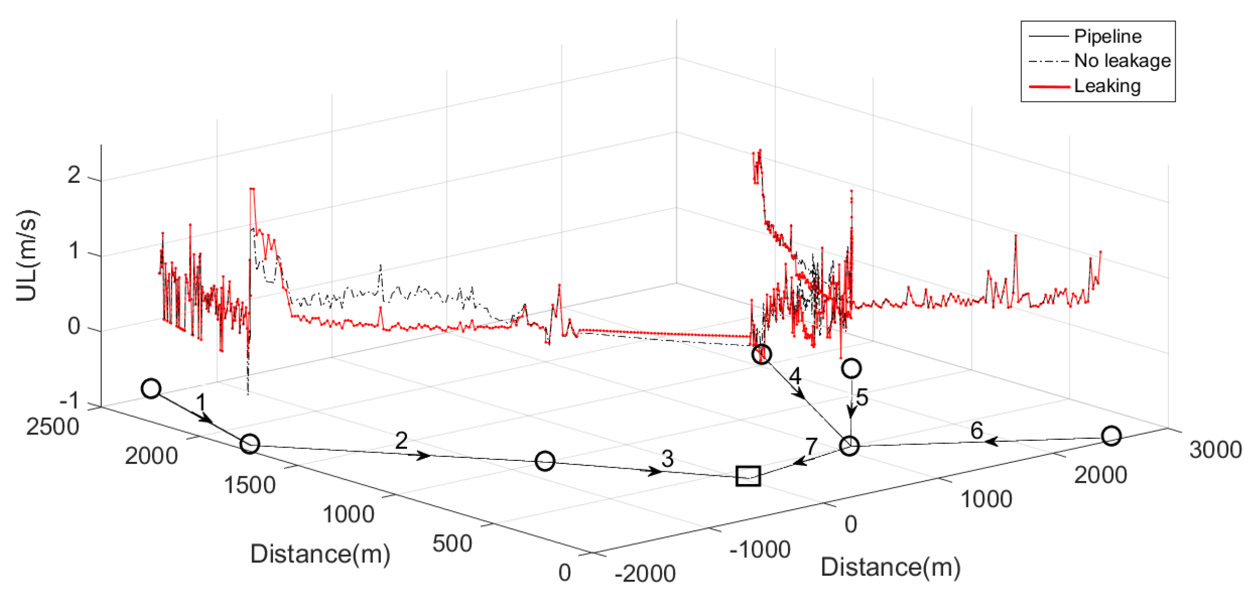
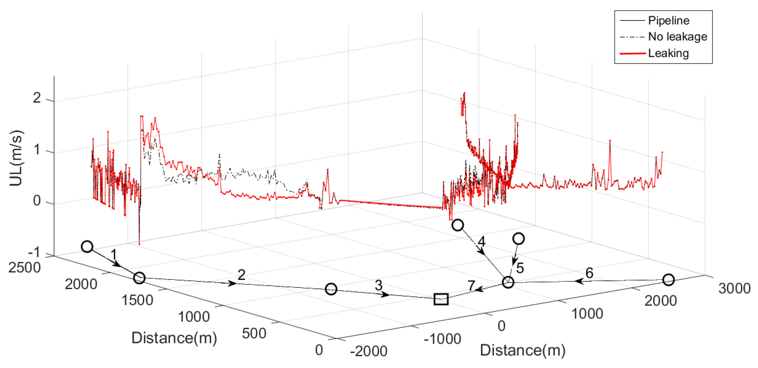
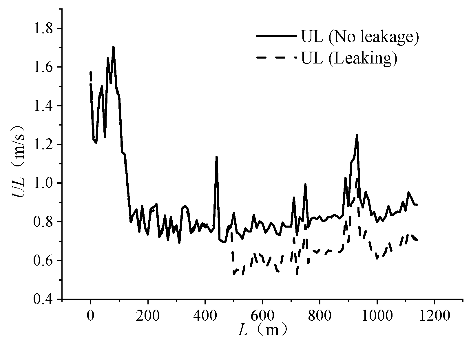
3.2.5. The Law of Liquid Flow Rate Change along the Pipeline

The change rule of the liquid flow rate of the pipe network before and after the leakage of pipe section 4 and pipe section 7 is shown in Figure 22 and Figure 23. The liquid flow rate before and after the leak shows a downward trend, and the total change trend of the liquid flow rate after the leak is the same as before the leak.

Figure 22. Change in liquid flow rate in pipeline network before and after leakage happened in pipe section 4.

Figure 22. Change in liquid flow rate in pipeline network before and after leakage happened in pipe section 4.

Figure 23. Change in liquid flow rate in pipeline network before and after leakage happened in pipe section 7.

Figure 23. Change in liquid flow rate in pipeline network before and after leakage happened in pipe section 7.

3.3. Identify Leaking Pipe Section Based on Pressure Changes

After a pipeline leak occurs, the parameters of the pipeline network will change accordingly. According to the pressure changes in the pipeline network, it can be seen that the pressure changed in the leaking pipe section are significantly higher than those of other non-leaking pipe sections. And the gas flow rate of the leaking pipe section will undergo an obvious sudden change after pipe section 4 or pipe section 7 leaks. This allows a preliminary assessment of the leaking section of pipe.

It can be seen from Figure 24 that pipe section 4 intersects the horizontal axis first, indicating that the pressure of pipe section 4 decreases the fastest with time, which also verifies that pipe section 4 is a leaking pipe section. The amplitude of the pressure changes of pipe section 7 before and after the leak is the same as that of pipe section 4, which verifies the accuracy of identifying the leaking pipe section based on the pressure change amplitude.

It can be seen from Figure 25 that the pipe section 7 and the horizontal axis intersect first, indicating that the pipe section 7 is a leaking pipe section, which also verifies that the leaking pipe section can be identified based on the speed of pressure change with time before and after the leak. At the same time, from the intersection of each pipe section with the abscissa, it can be seen that when pipe section 4 leaks, the pressure starts to drop 31.5% earlier than the other non-leaking pipe sections. When pipe section 7 leaks, the pressure starts to drop 20.7% earlier than other non-leaking pipe sections. It can be concluded that the time at which the pressure of the leaking pipe section starts to drop is more than 20% earlier than that of the non-leaking pipe section according to the analysis.

4. Conclusions

As this shale gas is a water-bearing (wet) shale gas, it flows in a gas–liquid two-phase flow in the pipeline network. As the gas pipeline is a very complex, non-linear, time-varying system, it is difficult to achieve satisfactory results using traditional methods for leak detection in pipeline networks. The use of the single-point leakage parameter change law of the pipe network to identify the leaking pipe sections in the pipe network is of great importance for maintaining pipeline safety, protecting human life and property safety, saving energy and reducing environmental pollution. Therefore, the accuracy of the pipe network leakage identification method based on the pressure drop rate model is effective to achieve the desired effect. Based on detailed theoretical research and actual field conditions, the following main conclusions can be drawn:

(1) By analyzing the law of change before and after leakage of these parameters such as pressure, temperature, liquid holdup, and gas-liquid flow rate, it is found that the pressure at the leak point in the leaking section of pipe changes suddenly. In addition, the pressure of the leaking section of pipe changes more than other non-leaking sections of pipe, which can help to identify leaking sections of pipe in the network early on.

(2) Based on the example of gas–liquid two-phase flow pipe network, the pressure change rate model is used to make the pressure change amplitude curve after leakage, which can identify the leakage pipe section more quickly and accurately.

(3) The statistical data of the shale gas gathering and transportation network verified the correctness of the method of identifying the leaking pipe section using the proposed method, where the start time of the pressure drop of the leaking pipe section is more than 20% earlier than the non-leaking pipe section.

References

1. Kumar, P.; Mohapatra, P.K. Simple graphical method for detection of a partial blockage or leak in a single pipeline. J. Press. Vessel Technol. 2021, 143, 054501. [Google Scholar] [CrossRef]
2. Qian, F.; Hu, M. Numerical simulation of leakage flow field and acoustic characteristics for safety valve. In MATEC Web of Conferences; EDP Sciences: Les Ulis, France, 2021; Volume 336, p. 01007. [Google Scholar]
3. Yang, L.; Guo, Y.; Gao, S. Multi-leak detection in pipeline based on optical fiber detection. Optik 2020, 220, 164996. [Google Scholar] [CrossRef]
4. Kim, H.J.; Shin, H.Y.; Pyeon, C.H.; Kim, S.; Lee, B. Fiber-optic humidity sensor system for the monitoring and detection of coolant leakage in nuclear power plants. Nucl. Eng. Technol. 2020, 52, 1689–1696. [Google Scholar] [CrossRef]
5. Quy, T.B.; Kim, J.M. Real-Time Leak Detection for a Gas Pipeline Using ak-NN Classifier and Hybrid AE Features. Sensors 2021, 21, 367. [Google Scholar] [CrossRef] [PubMed]
6. Wu, Q.; Lee, C.M. A modified leakage localization method using multilayer perceptron neural networks in a pressurized gas pipe. Appl. Sci. 2019, 9, 1954. [Google Scholar] [CrossRef]
7. Kabaasha, A.M.; Piller, O.; van Zyl, J.E. Incorporating the modified orifice equation into pipe network solvers for more realistic leakage modeling. J. Hydraul. Eng. 2018, 144, 04017064. [Google Scholar] [CrossRef]
8. Li, H.; Li, H.; Pei, H.; Li, Z. Leakage detection of HVAC pipeline network based on pressure signal diagnosis. In Building Simulation; Tsinghua University Press: Beijing, China, 2019; Volume 12, pp. 617–628. [Google Scholar]
9. Van der Walt, J.C.; Heyns, P.S.; Wilke, D.N. Pipe network leak detection: Comparison between statistical and machine learning techniques. Urban Water J. 2018, 15, 953–960. [Google Scholar] [CrossRef]
10. Liu, C.-W.; Li, Y.-X.; Yan, Y.-K.; Fu, J.-T.; Zhang, Y.-Q. A new leak location method based on leakage acoustic waves for oil and gas pipelines. J. Loss Prev. Process Ind. 2015, 35, 236–246. [Google Scholar] [CrossRef]
11. Rai, A.; Kim, J.M. A novel pipeline leak detection approach independent of prior failure information. Measurement 2021, 167, 108284. [Google Scholar] [CrossRef]
12. Oyedeko, K.F.K.; Balogun, H.A. Modeling and simulation of a leak detection for oil and gas pipelines via transient model: A case study of the Niger delta. J. Energy Technol. Policy 2015, 5, 16–27. [Google Scholar]
13. Lukonge, A.B.; Cao, X.; Pan, Z. Experimental study on leak detection and location for gas pipelines based on acoustic waves using improved Hilbert–Huang transform. J. Pipeline Syst. Eng. Pract. 2021, 12, 04020072. [Google Scholar] [CrossRef]
14. Sarkamaryan, S.; Haghighi, A.; Adib, A. Leakage detection and calibration of pipe networks by the inverse transient analysis modified by Gaussian functions for leakage simulation. J. Water Supply Res. Technol.-AQUA 2018, 67, 404–413. [Google Scholar] [CrossRef]
15. Aida-zade, K.R.; Ashrafova, Y.R. Numerical solution of inverse problem on determination of leakage for unsteady flow in a pipeline network. IFAC-Pap. 2018, 51, 21–26. [Google Scholar] [CrossRef]
16. Jia, W.; Wu, X.; Li, C.; He, Y. Characteristic analysis of a non-equilibrium thermodynamic two-fluid model for natural gas liquid pipe flow. J. Nat. Gas Sci. Eng. 2017, 40, 132–140. [Google Scholar] [CrossRef]
17. Coelho, R.C.; Ilha, A.; Doria, M.M.; Pereira, R.M.; Aibe, V.Y. Lattice Boltzmann method for bosons and fermions and the fourth-order Hermite polynomial expansion. Phys. Rev. E 2014, 89, 043302. [Google Scholar] [CrossRef] [PubMed]
18. Sun, J.; Li, Y.; Liang, Y. Research progress on leakage rate models for gas pipelines. Oil Gas Storage Transp. 2020, 39, 512–518. [Google Scholar]
19. Jin, J. Numerical Simulation Study on Leakage and Diffusion of Buried Gas Pipelines. Master’s Thesis, Zhejiang Ocean University, Zhoushan, China, 2021. [Google Scholar]
20. Zhang, S.; Zhang, Y.; Sheng, H.; Wei, P.; Wang, T. A Distributed Optical Fiber Thermal Pipeline Leakage Monitoring Experimental System and Implementation Method. CN115164116B, 30 December 2022. [Google Scholar]
21. Cui, Z.; Tian, L.; Duan, P.; Li, L.; Li, Y.; Liu, C. Setting of pressure drop rate threshold for cut-off valves in mixed hydrogen natural gas pipelines. Oil Gas Storage Transp. 2021, 40, 1293–1298. [Google Scholar]
22. Liu, C. Research on Sound Wave Generation and Propagation Characteristics of Gas Pipeline Leakage. Ph.D. Thesis, China University of Petroleum (East China), Qingdao, China, 2016. [Google Scholar]
Figure 1. Topological structure diagram of shale gas gathering and transportation pipeline network and leakage schematic diagram of pipeline section 1.
Energies 17 02464 g001
Figure 2. Pressure variation amplitude curve of the pipe section with leaked point after leakage.
Energies 17 02464 g002
Figure 3. Single point leakage model of pipe section 4 or pipe section 7.
Energies 17 02464 g003
Figure 4. Law of pressure change before and after leakage of pipe section 4.
Energies 17 02464 g004
Figure 5. Law of pressure change before and after leakage of pipe section 7.
Energies 17 02464 g005
Figure 6. Temperature changes before and after leakage in pipe section 4.
Energies 17 02464 g006
Figure 7. Temperature changes before and after leakage in pipe section 7.
Energies 17 02464 g007
Figure 8. Changes in liquid holdup before and after leakage in pipe section 4.
Energies 17 02464 g008
Figure 9. Changes in liquid holdup before and after leakage in pipe section 7.
Energies 17 02464 g009
Figure 10. Changes in gas flow velocity before and after leakage in pipe section 4.
Energies 17 02464 g010
Figure 11. Changes in gas flow velocity before and after leakage in pipe section 7.
Energies 17 02464 g011
Figure 12. Changes in liquid flow velocity before and after leakage in pipe section 4.
Energies 17 02464 g012
Figure 13. Changes in liquid flow velocity before and after leakage in pipe section 7.
Energies 17 02464 g013
Figure 24. Pressure variation amplitude of each pipe segment in the pipeline network with time after leakage of pipe segment 4.
Energies 17 02464 g024
Figure 25. Pressure variation amplitudes of each pipe segment in the pipeline network with time after leakage of pipe segment 7.
Energies 17 02464 g025