Comparison Study of the Wideband Oscillation Risk of MMC between Grid-Following and Grid-Forming Control

Abstract

Currently, research on the small-signal stability of grid-forming converters under two control modes, grid-following and grid-forming, mainly focuses on low-level converters. However, studies on the differences between grid-following modular multilevel converters (MMC) and grid-forming MMC are limited. A comprehensive analysis of the wideband oscillation risk differences in MMC-HVDC systems under these two control modes from the perspective of impedance characteristics is necessary. Therefore, based on the harmonic state-space (HSS) modeling theory, this article establishes wideband sequence impedance models for grid-forming and grid-following MMC. Subsequently, this article identifies key control parameters affecting the impedance characteristics of MMC under two control modes. The wideband oscillation risks of MMC-HVDC systems under both control modes are compared. The study indicates that when the grid strength weakens, grid-following MMC faces instability risks, while grid-forming MMC can maintain stability. In instances where high-frequency resonance peaks exist in the impedance of the grid, both control modes of MMC may face instability risks. Furthermore, by adjusting the obtained key control parameters of MMC, this article effectively suppresses the oscillation risk discussed above. Finally, the analysis results are verified through an electromagnetic transient simulation.

1. Introduction

Under grid-forming control, inverters can achieve self-synchronization while providing inertia and damping to the system [1,2]. This control mode has great potential in various applications such as flexible DC transmission [3,4], islanded power supply [5,6], and integration of renewable energy sources [7]. However, compared to grid-following control, grid-forming control also faces challenges such as high short-circuit currents [8,9]. Therefore, for a considerable period in the future, the coexistence of grid-following and grid-forming inverters, or the switching between control modes, will be the norm in new power systems. Revealing the wideband oscillation risks of inverters under both control modes is crucial for the safe and stable operation of the power grid.

Impedance analysis is one of the main methods for wideband oscillation analysis in flexible DC systems. The wideband impedance model, which is based on the small-signal linearized mathematical equations of converters, provides an intuitive reflection of the damping characteristics of converters at various frequencies. This model clarifies the oscillation mechanism and guides the design of oscillation suppression strategies. In the research on wideband impedance modeling of grid-forming converters: Ref. [10] establishes an impedance model for grid-connected converters, indicating that its virtual synchronization method partially avoids the interaction between the converter and weak grids caused by phase-locked loops (PLL), making it easier to maintain stability under weak grid conditions. Ref. [11] addresses the problem of sub-synchronous oscillations in weak grids of grid-forming direct-drive permanent magnet synchronous wind turbine units. It establishes a sequence impedance model of a grid-side converter based on harmonic linearization theory. By introducing dual-loop control, the grid-forming direct-drive wind turbine displays negative damping and capacitive traits in certain frequency ranges. This interaction with weak grids results in sub-synchronous oscillations. However, this paper does not compare the negative damping characteristics between grid-forming and grid-following control strategies. Ref. [12] analyzes the impact of grid-following and grid-forming energy storage converters on the stability of renewable energy stations. It establishes impedance models for grid-following and grid-forming energy storage converters. The results reveal that grid-forming energy storage converters are more conducive to enhancing the stability of renewable energy stations. However, due to the rapid increase in impedance magnitude of grid-forming converters in the mid-to-high frequency range, their damping effect on renewable energy units is weakened. This paper does not explicitly illustrate the mechanism through which grid-forming control reduces the risk of oscillations. Ref. [13] establishes impedance models of grid-forming converters for oscillation issues in wind and photovoltaic grid-connected systems under weak grids. It reveals the negative damping effect of outer-loop droop control and the positive damping effect of inner-loop control. Ref. [14] aims to clarify the mechanism and characteristics of improving oscillation stability with grid-forming control. It derives the impedance characteristics of grid-forming converters and their relationship with each control loop. Grid-forming converters display “positive resistance” due to reactive power control and voltage control. This mitigates the negative damping effects caused by grid-following converters, leading to enhanced stability of sub/super-synchronous oscillations in the system. Refs. [15,16] separately establish sequence impedance models for grid-following and grid-forming inverters. They analyze the significant effects of reactive power loop parameters and control delay on impedance negative damping. Their findings indicate that grid-forming control has a suppressing effect on sub/super-synchronous oscillations. These papers preliminarily identify the key control sections that affect the impedance characteristics of grid-forming converters but do not explicitly identify the specific key control parameters. Ref. [17] establishes impedance models with single-loop voltage control and dual-loop voltage-current control of grid-forming inverters to address high-frequency oscillation issues. It further analyzes the “passive characteristics” of typical control strategies based on the constraints of the phase angle of impedance. Ref. [18] establishes node admittance matrices considering grid-following and grid-forming converters, as well as transmission networks. It reveals the instability mechanism and the influence of multiple parameters on grid-following and grid-forming heterogeneous synchronous dynamics. Refs. [19,20] compare the characteristics of voltage control and current control virtual synchronous generators (VSG) as well as conventional grid-connected inverters based on impedance analysis. These findings suggest that voltage control type VSG is more adaptable to weak grids.

Currently, research on the wideband impedance characteristics of grid-forming converters mostly focuses on low-voltage converters, such as those used in wind turbines and photovoltaic systems. However, in flexible DC transmission projects that utilize modular multilevel converters (MMC) for high-voltage and large-capacity applications, the connection to weak grids poses a risk of instability. To mitigate this risk, the implementation of grid-forming control becomes crucial [21]. Nevertheless, the modular topology of MMC is characterized by low harmonic content independent of LC filtering, circulating currents, and long control delays. Studies have shown that the characteristic of long delay causes the negative damping of MMC impedance in a high-frequency range, which may lead to instability [22]. There are significant differences in wideband output impedance characteristics compared to low-voltage converters. Consequently, it is imperative to conduct a separate analysis of the influence of different control strategies on the wideband impedance characteristics of MMC [23,24,25].

In summary, current research on the stability of converters under the control of grid-following and grid-forming modes mainly focuses on low-voltage converters. However, comparative studies on the oscillation risks between grid-forming MMC and grid-following MMC are limited. Furthermore, the key factors affecting the impedance characteristics of grid-forming MMC remain unclear. The limitation of current research is summarized as

Table 1. Summary table of the literature.

Research	References	Limitation
Impedance modeling of grid-forming MMC	[10,11,12,19,20,21,22,23,24,25]	Studies about grid-forming control mostly focus on low-voltage converters. Research on grid-forming MMC are relatively limited.
Influencing factors of grid-forming converter impedance characteristics	[13,14,15,16,17,18]	Specific key control parameters affecting impedance characteristics are not clear.

.

Therefore, based on the harmonic state-space (HSS) theory, this article establishes sequence impedance models for grid-forming and grid-following MMC. The comparison and analysis of the two control modes’ impact on impedance characteristics are then conducted. Furthermore, utilizing the established sequence impedance model, this article identifies key control parameters affecting the wideband impedance characteristics of grid-forming MMC. Additionally, this article analyzes the wideband oscillation risks of MMC-HVDC systems when MMC adopts two different control modes. Subsequently, by adjusting the obtained key control parameters of MMC, this article effectively suppresses the oscillation risk discussed above. Finally, the accuracy of the established sequence impedance model, as well as the reliability of the stability analysis results, are validated through time-domain simulations.

2. Broadband Mathematical Modeling of MMC

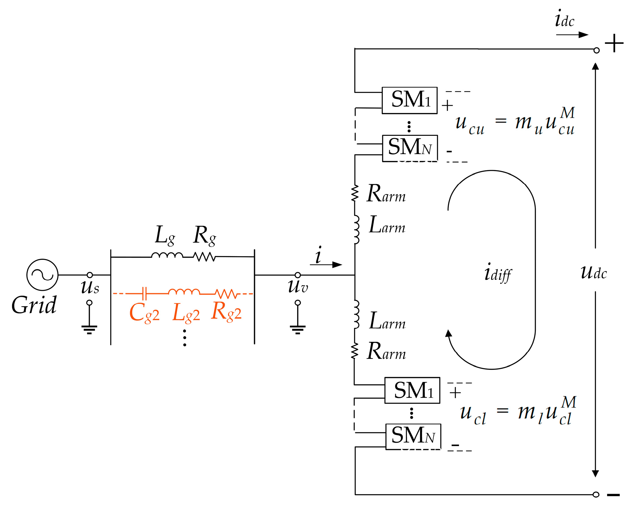
2.1. Configuration of MMC

Figure 1 illustrates the diagram of the single-phase bridge arm structure of MMC. u_v represents the AC terminal voltage of MMC. u_s represents the grid voltage. i represents the AC-side current. u_Cu and u_Cl are the upper and lower pole voltages. m_u and m_l are the corresponding modulation signals. $u_{\mathit{Cu}}^M$ and $u_{\mathit{Cl}}^M$ are the equivalent voltages of the upper and lower bridge arms. i_diff represents the differential-mode current. i_dc and u_dc are the DC-side current and voltage. R_arm and L_arm represent the equivalent resistance and equivalent inductance of the bridge arms, respectively. R_g and L_g represent the equivalent resistance and equivalent inductance of the grid, respectively. The impedance of the transformer can be integrated into the impedance of the power grid.

The average value model assumes consistent dynamic characteristics for all sub-modules and takes the sum of all capacitor voltages on each bridge arm as the system state variable. The average value model representing the dynamic behavior of a single-phase MMC is expressed as:

$$\frac{\mathrm{d}}{\mathrm{d}t}\left[\begin{array}{c}{i}_{diff}\\ i\\ u_{Cu}^M\\ u_{Cl}^M\end{array}\right]=\left[\begin{array}{llll}-\frac{R_{arm}}{L_{arm}}\hfill & 0\hfill & -\frac{m_u}{2L_{arm}}\hfill & -\frac{m_l}{2L_{arm}}\hfill \\ 0\hfill & -\frac{2R_{arm}}{L_{arm}}\hfill & \frac{m_u}{L_{arm}}\hfill & -\frac{m_l}{L_{arm}}\hfill \\ \frac{m_u}{C_{arm}}\hfill & -\frac{m_u}{2C_{arm}}\hfill & 0\hfill & 0\hfill \\ \frac{m_l}{C_{arm}}\hfill & \frac{m_l}{2C_{arm}}\hfill & 0\hfill & 0\hfill \end{array}\right]\left[\begin{array}{c}{i}_{diff}\\ i\\ u_{Cu}^M\\ u_{Cl}^M\end{array}\right]+\left[\begin{array}{cc}\frac{1}{2L_{arm}}& 0\\ 0& \frac{2}{L_{arm}}\\ 0& 0\\ 0& 0\end{array}\right]\left[\begin{array}{c}{u}_{dc}\\ u_v\end{array}\right]$$

(1)

where C_arm represents the equivalent capacitance of the bridge arm, which can be calculated as C_SM/N. C_SM represents the capacitance of each submodule and N represents the number of submodules in a single bridge arm.

The average model of MMC is a nonlinear time-periodic (NTP) model, which is difficult to analyze directly. The linear time-invariant (LTI) model of MMC is established using the harmonic state-space (HSS) modeling method, followed by the derivation of the small-signal impedance model for MMC.

2.2. Harmonic State-Space Modeling Theory

The state equation of MMC shown in Equation (1) can be expressed in the following form of NTP model:

$$\left\{\begin{array}{l}\frac{d\mathit{x}}{\mathit{dt}}=\mathit{f}(\mathit{x},\mathit{u})\hfill \\ \mathit{y}=\mathit{g}(\mathit{x},\mathit{u})\hfill \end{array}\right.$$

(2)

where x, u, and y represent the state vector, input vector, and output vector, respectively, while f and g are nonlinear algebraic functions.

By employing the HSS modeling method, the time-domain model is transformed into the harmonic domain in the authors’ previous work [26].

$$\left\{\begin{array}{l}(\mathrm{s}{\mathit{I}}_{\mathrm{X}}+\mathit{N})\widehat{\mathit{X}}={\mathit{A}}_{\mathrm{H}}\widehat{\mathit{X}}+{\mathit{B}}_{\mathrm{H}}\widehat{\mathit{U}}\hfill \\ \widehat{\mathit{Y}}={\mathit{C}}_{\mathrm{H}}\widehat{\mathit{X}}+{\mathit{D}}_{\mathrm{H}}\widehat{\mathit{U}}\hfill \end{array}\right.$$

(3)

The model of the MMC can be expressed as:

$$\Delta \dot{\mathit{x}}={\mathit{A}}_{\mathrm{Tx}}\Delta \mathit{x}+{\mathit{A}}_{\mathrm{Tz}}\Delta \mathit{z}+{\mathit{B}}_{\mathrm{T}}\Delta \mathit{u}$$

(4)

where the state variable $\Delta \mathit{x}={\left[\begin{array}{cccc}\Delta i_{\mathit{diff}}& \Delta i& \Delta u_{\mathit{Cu}}^M& \Delta u_{\mathit{Cl}}^M\end{array}\right]}^T$, input variable $\Delta \mathit{u}={\left[\begin{array}{cc}\Delta u_{\mathit{dc}}& \Delta u_v\end{array}\right]}^T$, and intermediate variable $\Delta \mathit{z}=\left[\begin{array}{cc}\Delta m_u& \Delta m_l\end{array}\right]$. The expressions for the coefficient matrices in Equation (4) are provided in Appendix A.

In the HSS model, the coefficient matrices can be represented as A_Hx = Γ(A_Tx)_,A_Hz = Γ(A_Tz), B_H = Γ(B_T). Therefore, these matrices are represented by complex Fourier coefficients of different harmonic orders, which are expressed in terms of amplitude and phase angle rather than time-varying signals. For instance, A_Hx1 and A_Hx−1, the two elements of A_Hx, are composed of the positive and negative sequence fundamental frequency components of A_Tx, respectively. These Fourier coefficients can be obtained through simulation or calculated using the method described in ref. [27]. Oscillation frequencies in current engineering applications are all below 2500 Hz. Within this frequency range, the inductance of reactors and the capacitance of capacitors can be considered constant. Therefore, the frequency-dependent effects of power electronic devices can be neglected in this article.

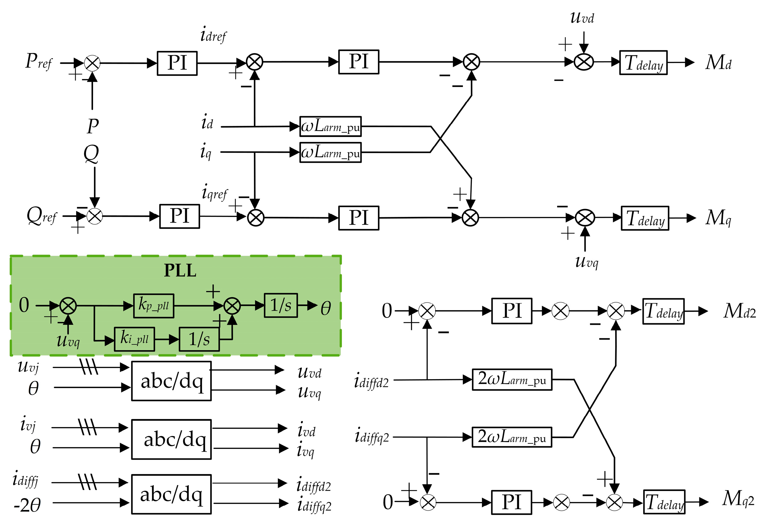
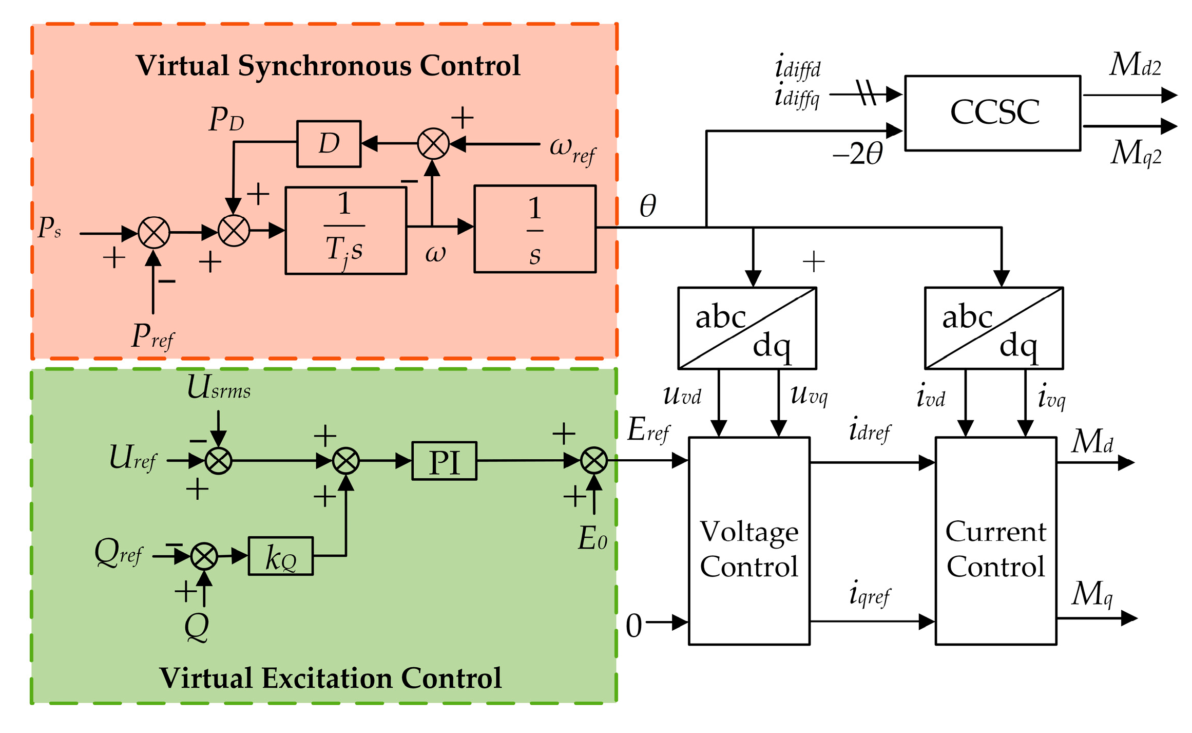
2.3. Broadband Impedance Model of Grid-Forming MMC

The open-loop impedance model of MMC serves as the basis for closed-loop impedance models under control. Therefore, this section illustrates the derivation process from the state equation to the open-loop impedance model by introducing the HSS modeling method.

In open-loop control conditions, the disturbance of the modulation signal is zero, hence ∆z = 0. Then, $\Delta \dot{\mathit{x}}={\mathit{A}}_{\mathrm{Tx}}\Delta \mathit{x}+{\mathit{B}}_{\mathrm{T}}\Delta \mathit{u}$, the simplified time-domain LTP equation can be transformed from the time domain to the harmonic domain. By letting the output variable be the state variable, i.e., $\widehat{\mathit{Y}}=\widehat{\mathit{X}}$, the harmonic input-output relationship can be expressed as:

$$\widehat{\mathit{Y}}={\mathit{H}}_{\mathrm{MMC}}^{\mathrm{tf}}\widehat{\mathit{U}}$$

(5)

The expression for the harmonic transfer matrix ${\mathit{H}}_{\mathrm{MMC}}^{\mathrm{tf}}$ can be found in Appendix A.

The definition of Y_pn11 is the MMCs sequence admittance when the third and higher harmonics are neglected. Clearly, Y_pn11 is a sub-matrix of ${\mathit{H}}_{\mathrm{MMC}}^{\mathrm{tf}}$. Considering the dynamics of the h-th higher harmonic, where the length of the column vectors $\widehat{\mathit{X}}$ and $\widehat{\mathit{U}}$ are 4 × (2h + 1) and 2 × (2h + 1), respectively, the fundamental frequency sequence admittance of the MMC is:

$${\mathit{Y}}_{\mathit{pn}}=\left[\begin{array}{cc}{H}_{\mathrm{MMC}}^{\mathrm{tf}}\left(4h+6,2h+4\right)& H_{\mathrm{MMC}}^{\mathrm{tf}}\left(4h+6,2h\right)\\ H_{\mathrm{MMC}}^{\mathrm{tf}}\left(4h-2,2h+4\right)& H_{\mathrm{MMC}}^{\mathrm{tf}}\left(4h-2,2h\right)\end{array}\right]$$

(6)

where $H_{\mathrm{MMC}}^{\mathrm{tf}}\left(i,j\right)$ denotes the element of matrix ${\mathit{H}}_{\mathrm{MMC}}^{\mathrm{tf}}$ in the i-th row and the j-th column. When higher harmonics are considered in the HSS model, higher harmonic Fourier series coefficients need to be added to all harmonic transfer matrices using a similar modeling approach. Based on the fundamental frequency sequence admittance of the MMC, the open-loop sequence impedance of the MMC can be obtained by matrix inversion.

To study the oscillation risk of the MMC-HVDC system under grid-forming control and compare it with grid-following control, this article selects conventional dual-loop control with constant PQ as the outer loop, provided by a phase-locked loop to supply phase, as a typical grid-following control method. For the grid-forming control method, it selects virtual synchronous control with virtual excitation control (internal potential amplitude calculation) providing voltage control’s preference value and virtual rotor motion equations (virtual angle generation) providing phase. The control block diagrams for both control modes are shown in Figure 2 and Figure 3, respectively.

Due to the consistency of the current control, circulating current suppression control (CCSC), and modulation section under both control modes, this article will briefly introduce the basic method of closed-loop impedance modeling and the modeling process of obtaining phase under grid-forming control. In the following derivation, only textual explanations will be provided for certain matrices in the equations. The specific expressions can be found in the author’s previous work [26].

When the controller is added, Δz ≠ 0, it is necessary to incorporate the controller dynamics into the system dynamic equations. For the convenience of implementing the impedance model in computer programming, the HSS model of the MMC is divided into four parts:

$$\left\{\begin{array}{l}\left(\mathrm{s}\mathit{I}+\mathit{N}\right)\widehat{\mathit{X}}={\mathit{A}}_{\mathrm{Hx}}\widehat{\mathit{X}}+{\mathit{A}}_{\mathrm{Hz}}\widehat{\mathit{Z}}+{\mathit{B}}_{\mathrm{H}}\widehat{\mathit{U}}\hfill \\ \widehat{\mathit{Z}}={\mathit{C}}_{\mathrm{Hm}1}{\widehat{\mathit{M}}}_1+{\mathit{C}}_{\mathrm{Hm}2}{\widehat{\mathit{M}}}_2\hfill \\ {\widehat{\mathit{M}}}_1={\mathit{D}}_{\mathrm{H}1}\widehat{\mathit{X}}+{\mathit{E}}_{\mathrm{H}1}\widehat{\mathit{U}}\hfill \\ {\widehat{\mathit{M}}}_2={\mathit{D}}_{\mathrm{H}2}\widehat{\mathit{X}}+{\mathit{E}}_{\mathrm{H}2}\widehat{\mathit{U}}\hfill \end{array}\right.$$

(7)

The first equation in (7) represents the dynamics of the electrical system. The intermediate variables $\widehat{\mathit{Z}}$ are the modulation signals for the upper and lower bridge arms. The second equation in (7) represents the transformation of the modulation signals. ${\widehat{\mathit{M}}}_1$ and ${\widehat{\mathit{M}}}_2$ represent the modulation signals outputted by the main control and CCSC, respectively. Based on the relationship between the modulation signals of the upper and lower bridge arms and the controller modulation signals, the expressions for the constant matrices C_Hm1 and C_Hm2 can be obtained [23]. And $\widehat{\mathit{Z}}$ can be calculated from ${\widehat{\mathit{M}}}_1$ and ${\widehat{\mathit{M}}}_2$. The third and fourth equations in (7) represent the dynamics of the main controller and CCSC, respectively. Therefore, the specific expressions of D_H1, E_H1, D_H2, and E_H2 depend on the control method used by the MMC. After obtaining the expressions of the transfer function matrices in Equation (7), the transfer function matrix from $\widehat{\mathit{U}}$ to $\widehat{\mathit{X}}$ can be written as:

$$\begin{array}{l}{\mathit{H}}_{\mathrm{MMC}}^{\mathrm{tf}}={\left(\mathrm{s}\mathit{I}+\mathit{N}-{\mathit{A}}_{\mathrm{Hx}}-{\mathit{A}}_{\mathrm{Hz}}\left({\mathit{C}}_{\mathrm{Hm}1}{\mathit{D}}_{\mathrm{H}1}+{\mathit{C}}_{\mathrm{Hm}2}{\mathit{D}}_{\mathrm{H}2}\right)\right)}^{-1}·\\ \left({\mathit{A}}_{\mathrm{Hz}}\left({\mathit{C}}_{\mathrm{Hm}1}{\mathit{E}}_{\mathrm{H}1}+{\mathit{C}}_{\mathrm{Hm}2}{\mathit{E}}_{\mathrm{H}2}\right)+{\mathit{B}}_{\mathrm{H}}\right)\end{array}$$

(8)

Once the expressions for ${\mathit{H}}_{\mathrm{MMC}}^{\mathrm{tf}}$ are obtained, the derivation process for the open-loop impedance is consistent with the process outlined in Equation (6), yielding the fundamental frequency sequence admittance and impedance of the MMC.

Next, this paper derives the expressions for D_H1, E_H1, D_H2, and E_H2 under grid-forming control, obtaining the closed-loop broadband impedance model of grid-forming MMC.

The key disparity distinguishing the control system of the MMC under grid-forming control from that under grid-following control lies in the provision of phase information by the virtual rotor motion equation. Therefore, the crucial step in establishing the wideband impedance model of the grid-forming MMC is to express the HSS form of the virtual angle generation.

To illustrate the process of obtaining the phase through virtual synchronous control, the virtual rotor dynamics equation under grid-forming control can be written as:

$$\left\{\begin{array}{l}\frac{\mathrm{d}\omega }{\mathrm{d}t}=\frac{1}{T_j}\left(P_s-P_{ref}+D\left(100\mathsf{\pi }-\omega \right)\right)\hfill \\ \frac{\mathrm{d}\theta }{\mathrm{d}t}=\omega \hfill \end{array}\right.$$

(9)

where T_j represents the inertia time constant, D stands for the damping coefficient, and ω denotes the virtual angular velocity used in control. P_s represents the output active power and P_ref represents the reference value of active power.

Linearizing Equation (9) and transforming it into the frequency domain, its HSS form can be expressed as:

$$\begin{array}{l}{{\mathit{G}}^{\prime }}_{\mathrm{HPLL}}\widehat{\mathit{\theta }}=\left[\begin{array}{cc}{\mathit{U}}_{\mathrm{Hvd}}^{\mathrm{c}}& {\mathit{U}}_{\mathrm{Hvq}}^{\mathrm{c}}\end{array}\right]\left[\begin{array}{c}{\widehat{\mathit{I}}}_{\mathrm{d}}^{\mathrm{c}}\\ {\widehat{\mathit{I}}}_{\mathrm{q}}^{\mathrm{c}}\end{array}\right]+\left[\begin{array}{cc}{\mathit{I}}_{\mathrm{Hd}}^{\mathrm{c}}& {\mathit{I}}_{\mathrm{Hq}}^{\mathrm{c}}\end{array}\right]\left[\begin{array}{c}{\widehat{\mathit{U}}}_{\mathrm{vd}}^{\mathrm{c}}\\ {\widehat{\mathit{U}}}_{\mathrm{vq}}^{\mathrm{c}}\end{array}\right]\\ =\left[\begin{array}{cc}{\mathit{U}}_{\mathrm{Hvd}}^{\mathrm{c}}& {\mathit{U}}_{\mathrm{Hvq}}^{\mathrm{c}}\end{array}\right]\left(\frac{{\mathit{P}}_{\mathrm{H}}}{U_{\mathrm{base}}}\left[\begin{array}{c}{\hat{I}}_a\\ {\hat{I}}_b\\ {\hat{I}}_c\end{array}\right]+\left[\begin{array}{c}{\mathit{I}}_{\mathrm{Hq}}^{\mathrm{c}}\\ -{\mathit{I}}_{\mathrm{Hd}}^{\mathrm{c}}\end{array}\right]\widehat{\mathit{\theta }}\right)+\left[\begin{array}{cc}{\mathit{I}}_{\mathrm{Hd}}^{\mathrm{c}}& {\mathit{I}}_{\mathrm{Hq}}^{\mathrm{c}}\end{array}\right]\left(\frac{{\mathit{P}}_{\mathrm{H}}}{{\mathit{U}}_{\mathrm{base}}}\left[\begin{array}{c}{\widehat{\mathit{U}}}_{\mathrm{v}a}^{\mathrm{c}}\\ {\widehat{\mathit{U}}}_{\mathrm{v}b}^{\mathrm{c}}\\ {\widehat{\mathit{U}}}_{\mathrm{v}c}^{\mathrm{c}}\end{array}\right]+\left[\begin{array}{c}{\mathit{U}}_{\mathrm{Hvq}}^{\mathrm{c}}\\ -{\mathit{U}}_{\mathrm{Hvd}}^{\mathrm{c}}\end{array}\right]\widehat{\mathit{\theta }}\right)\\ =\left[\begin{array}{cc}{\mathit{U}}_{\mathrm{Hvd}}^{\mathrm{c}}& {\mathit{U}}_{\mathrm{Hvq}}^{\mathrm{c}}\end{array}\right]\frac{{\mathit{P}}_{\mathrm{H}}}{U_{\mathrm{base}}}\left[\begin{array}{c}{\hat{I}}_a\\ {\hat{I}}_b\\ {\hat{I}}_c\end{array}\right]+\left[\begin{array}{cc}{\mathit{I}}_{\mathrm{Hd}}^{\mathrm{c}}& {\mathit{I}}_{\mathrm{Hq}}^{\mathrm{c}}\end{array}\right]\frac{{\mathit{P}}_{\mathrm{H}}}{U_{\mathrm{base}}}\left[\begin{array}{c}{\widehat{\mathit{U}}}_{\mathrm{v}a}^{\mathrm{c}}\\ {\widehat{\mathit{U}}}_{\mathrm{v}b}^{\mathrm{c}}\\ {\widehat{\mathit{U}}}_{\mathrm{v}c}^{\mathrm{c}}\end{array}\right]\end{array}$$

(10)

where, ${{\mathit{G}}^{\prime }}_{\mathrm{HPLL}}=\mathrm{diag}\left(\cdots ,\left(\mathrm{s}-j{\omega }_1\right)\left(T_j\left(\mathrm{s}-j{\omega }_1\right)-D\right),\mathrm{s}\left(T_j\mathrm{s}-D\right),\left(\mathrm{s}+j{\omega }_1\right)\left(T_j\left(\mathrm{s}+j{\omega }_1\right)-D\right),\cdots \right)$

The expression for $\widehat{\mathit{\theta }}$ can be expressed as:

$$\widehat{\mathit{\theta }}=\underset{{\mathit{G}}_{\mathrm{HPLL}}^{\mathsf{\theta }\mathrm{i}}}{\underbrace{{\left({{\mathit{G}}^{\prime }}_{\mathrm{HPLL}}\right)}^{-1}\cdot \left[\begin{array}{cc}{\mathit{U}}_{\mathrm{Hvd}}^{\mathrm{c}}& {\mathit{U}}_{\mathrm{Hvq}}^{\mathrm{c}}\end{array}\right]\frac{{\mathit{P}}_{\mathrm{H}}}{U_{\mathrm{base}}}}}\left[\begin{array}{c}{\hat{I}}_a\\ {\hat{I}}_b\\ {\hat{I}}_c\end{array}\right]+\underset{{\mathit{G}}_{\mathrm{HPLL}}^{\mathsf{\theta }\mathrm{uv}}}{\underbrace{{\left({{\mathit{G}}^{\prime }}_{\mathrm{HPLL}}\right)}^{-1}\cdot \left[\begin{array}{cc}{\mathit{I}}_{\mathrm{Hd}}^{\mathrm{c}}& {\mathit{I}}_{\mathrm{Hq}}^{\mathrm{c}}\end{array}\right]\frac{{\mathit{P}}_{\mathrm{H}}}{U_{\mathrm{base}}}}}\left[\begin{array}{c}{\widehat{\mathit{U}}}_{\mathrm{v}a}^{\mathrm{c}}\\ {\widehat{\mathit{U}}}_{\mathrm{v}b}^{\mathrm{c}}\\ {\widehat{\mathit{U}}}_{\mathrm{v}c}^{\mathrm{c}}\end{array}\right]$$

(11)

According to the expression of $\widehat{\mathit{\theta }}$, we can derive the coordinate transformation equations for each variable, and subsequently deduce the HSS forms of virtual excitation control, voltage control, and current control. The detailed derivation process is provided in Appendix C.

Finally, we can obtain the expressions for D_H1 and E_H1:

$$\left\{\begin{array}{l}{\mathit{D}}_{\mathrm{H}1}=\left[\begin{array}{ccc}\mathit{I}& \mathbf{0}& \mathbf{0}\end{array}\right]\left({\mathit{G}}_{\mathrm{Hcd}}^{\mathrm{m}-1}\left({\mathit{G}}_{\mathrm{m}}^{\mathrm{i}}\left({\mathit{G}}_{\mathrm{Hcd}}^{\mathrm{i}}+{\mathit{G}}_{\mathrm{HPLLi}}^{\mathrm{i}}\right)+{\mathit{G}}_{\mathrm{m}}^{\mathrm{uv}}{\mathit{G}}_{\mathrm{HPLLi}}^{\mathrm{uv}}\right)+{\mathit{G}}_{\mathrm{HPLLi}}^{\mathrm{m}-1}\right){\mathit{S}}_{\mathrm{i}}\hfill \\ {\mathit{E}}_{\mathrm{H}1}=\left[\begin{array}{ccc}\mathit{I}& \mathbf{0}& \mathbf{0}\end{array}\right]\left({\mathit{G}}_{\mathrm{Hcd}}^{\mathrm{m}-1}\left({\mathit{G}}_{\mathrm{m}}^{\mathrm{i}}{\mathit{G}}_{\mathrm{HPLLuv}}^{\mathrm{i}}+{\mathit{G}}_{\mathrm{m}}^{\mathrm{uv}}\left({\mathit{G}}_{\mathrm{Hcd}}^{\mathrm{uv}}+{\mathit{G}}_{\mathrm{HPLLuv}}^{\mathrm{uv}}\right)\right)+{\mathit{G}}_{\mathrm{HPLLuv}}^{\mathrm{m}-1}\right){\mathit{S}}_{\mathrm{uv}}\hfill \end{array}\right.$$

(12)

Since the dynamics of $\widehat{\mathit{\theta }}$ depend on the ${\widehat{\mathit{U}}}_{\mathrm{vdq}}^{\mathrm{c}}$ and ${\widehat{\mathit{I}}}_{\mathrm{dq}}^{\mathrm{c}}$ in Appendix C, an additional coefficient matrix ${\widehat{\mathit{I}}}_{\mathrm{dq}}^{\mathrm{c}}$ needs to be added to the HSS representation of the current loop controller, denoted as F_H2. By substituting the coordinate transformation equations of each variable into the expression for the CCSC dynamics, the expressions for D_H2, E_H2, and F_H2 can be furtherly obtained:

$$\left\{\begin{array}{l}{\mathit{D}}_{\mathrm{H}2}=\left[\begin{array}{ccc}\mathit{I}& \mathbf{0}& \mathbf{0}\end{array}\right]{\mathit{G}}_{\mathrm{Hcd}}^{\mathrm{m}-2}\left({\mathit{G}}_{\mathrm{Hccsc}2}-{\mathit{G}}_{\mathrm{Hccsc}1}\right){\mathit{G}}_{\mathrm{Hcd}}^{\mathrm{idiff}}{\mathit{S}}_{\mathrm{idiff}}\hfill \\ {\mathit{E}}_{\mathrm{H}2}=\left[\begin{array}{ccc}\mathit{I}& \mathbf{0}& \mathbf{0}\end{array}\right]\left({\mathit{G}}_{\mathrm{Hcd}}^{\mathrm{m}2-1}\left({\mathit{G}}_{\mathrm{Hccsc}2}-{\mathit{G}}_{\mathrm{Hccsc}1}\right){\mathit{G}}_{\mathrm{HPLLuv}}^{\mathrm{idiff}}+{\mathit{G}}_{\mathrm{HPLLuv}}^{\mathrm{m}2-1}\right){\mathit{S}}_{\mathrm{uv}}\hfill \\ {\mathit{F}}_{\mathrm{H}2}=\left[\begin{array}{ccc}\mathit{I}& \mathbf{0}& \mathbf{0}\end{array}\right]\left({\mathit{G}}_{\mathrm{Hcd}}^{\mathrm{m}2-1}\left({\mathit{G}}_{\mathrm{Hccsc}2}-{\mathit{G}}_{\mathrm{Hccsc}1}\right){\mathit{G}}_{\mathrm{HPLLi}}^{\mathrm{idiff}}+{\mathit{G}}_{\mathrm{HPLLi}}^{\mathrm{m}2-1}\right){\mathit{S}}_i\hfill \end{array}\right.$$

(13)

The transfer function matrix from $\widehat{\mathit{U}}$ to $\widehat{\mathit{X}}$ can be represented as:

$$\begin{array}{l}{\mathit{H}}_{\mathrm{MMC}}^{\mathrm{tf}}={\left(\mathrm{s}\mathit{I}+\mathit{N}-{\mathit{A}}_{\mathrm{Hx}}-{\mathit{A}}_{\mathrm{Hz}}\left({\mathit{C}}_{\mathrm{Hm}1}{\mathit{D}}_{\mathrm{H}1}+{\mathit{C}}_{\mathrm{Hm}2}{\mathit{D}}_{\mathrm{H}2}+{\mathit{C}}_{\mathrm{Hm}2}{\mathit{F}}_{\mathrm{H}2}\right)\right)}^{-1}\cdot \\ \left({\mathit{A}}_{\mathrm{Hz}}\left({\mathit{C}}_{\mathrm{Hm}1}{\mathit{E}}_{\mathrm{H}1}+{\mathit{C}}_{\mathrm{Hm}2}{\mathit{E}}_{\mathrm{H}2}\right)+{\mathit{B}}_{\mathrm{H}}\right)\end{array}$$

(14)

Based on the expression for ${\mathit{H}}_{\mathrm{MMC}}^{\mathrm{tf}}$, the fundamental frequency sequence admittance and sequence impedance of MMC under grid-forming control mode can be obtained using Equation (6). The abbreviations table explaining the symbols appearing in the modeling process of this article are as shown in

Table A1. Abbreviations table explaining the symbols in the modeling process.

Symbols	Explanation
uv	AC terminal voltage of MMC
us	Grid voltage
i	AC-side current
uCu uCl	Upper and lower pole voltages
mu ml	Modulation signals of upper and lower bridge arms
$u_{\mathit{Cu}}^M$ $u_{\mathit{Cl}}^M$	Equivalent voltages of the upper and lower bridge arms
idiff	Differential-mode current
idc udc	DC-side current and voltage
Rarm Larm	Equivalent resistance and inductance of the bridge arms
Rg Lg	Equivalent resistance and inductance of the grid
Carm	Equivalent capacitance of the bridge arm
Tj	Inertia time constant
D	Damping coefficient
ω	Virtual angular velocity
θ	Virtual phase angle
Δx, Δu, Δy	State vector, input vector, and output vector
AHx, AHz, BH	Coefficient matrices
Ubase Ibase	Base values for voltage and current
PH	Matrix representing the dynamic of coordinate transformation
GHpll	Matrix representing the dynamic of PLL
$\widehat{\mathit{\theta }}$	Matrix representing the dynamic of virtual phase angle
${\widehat{\mathit{U}}}_{\mathrm{vdq}}^{\mathrm{c}}$ ${\widehat{\mathit{I}}}_{\mathrm{dq}}^{\mathrm{c}}$	Matrix representing the dynamic of output voltage and current
h	Highest harmonic order
$\widehat{\mathit{Z}}$	Modulation signals matrix for the upper and lower bridge arms
${\widehat{\mathit{M}}}_1$ ${\widehat{\mathit{M}}}_2$	Modulation signals matrix outputted by the main control and CCSC
${\mathit{H}}_{\mathrm{MMC}}^{\mathrm{tf}}$	Harmonic transfer matrix
Ypn11	MMCs sequence admittance matrix

.

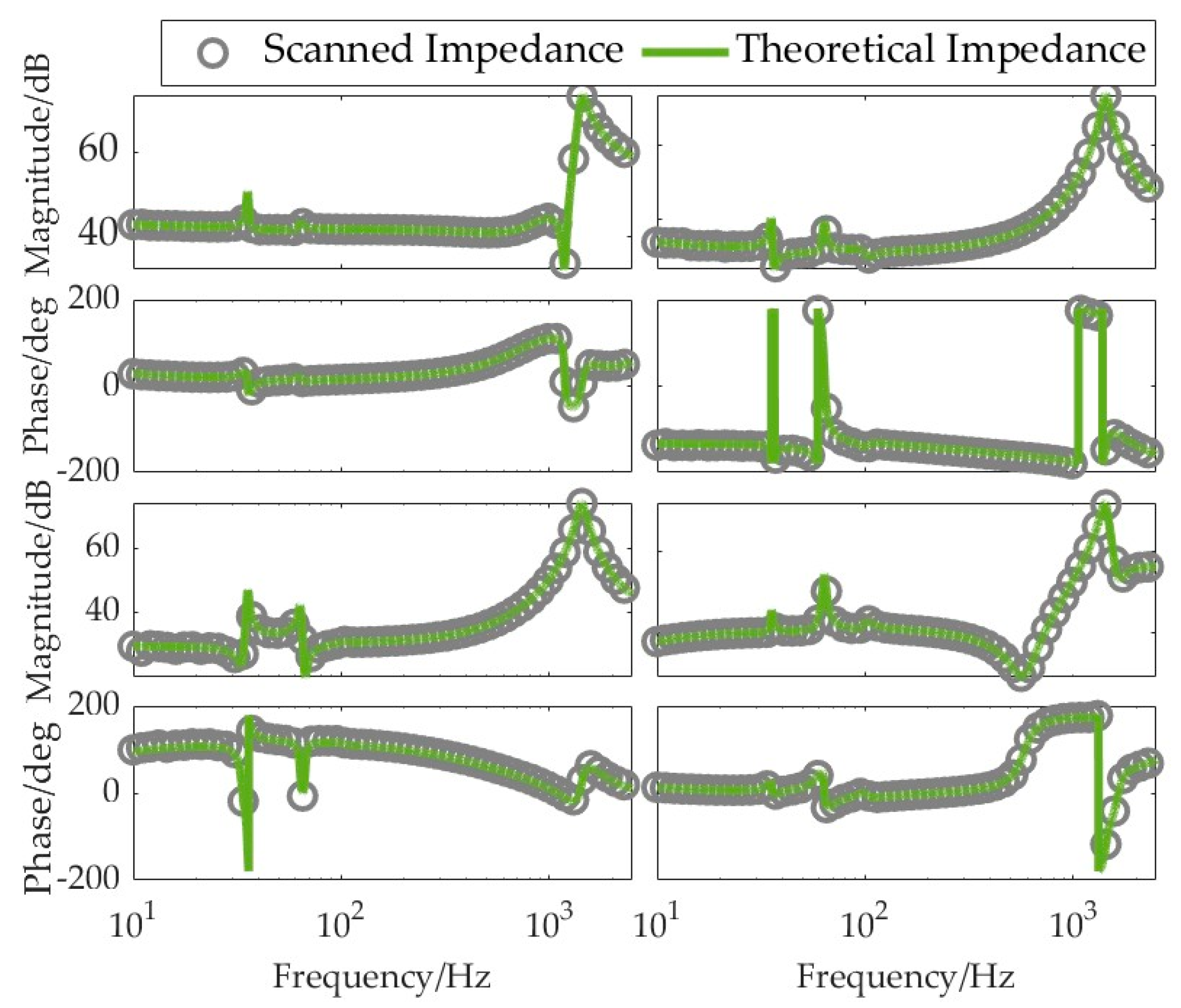
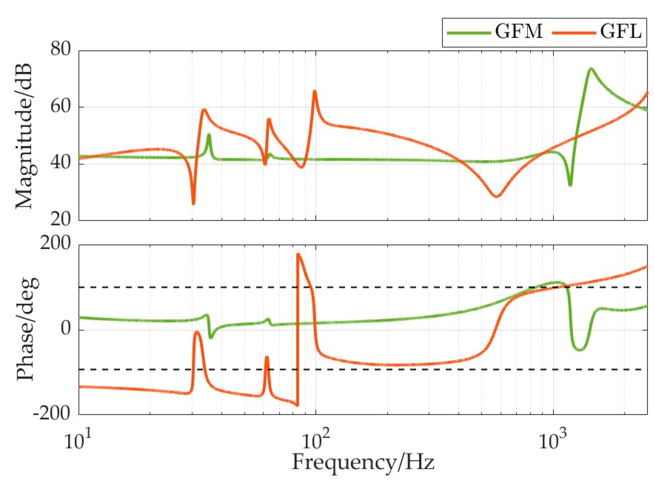
2.4. Verification of the Broadband Impedance Model

In order to compare the impedance characteristics of the grid-forming MMC with those of the grid-following MMC, an impedance model for the grid-following MMC is also established using the HSS modeling method in this article. The detailed derivation process can be found in Appendix B of this article.

To validate the accuracy of the theoretical models, three-phase transient electromagnetic simulation models of the MMC are constructed in MATLAB/Simulink, with specific parameters detailed in

Table A2. Electrical parameters of the simulation model.

Grid		MMC
Quantity	Value	Quantity	Value
Rated frequency of the system f1 (Hz)	50	Rated capacity of MMC Sbase (MVA)	1500
Rated voltage of the system us (kV)	437	Transmission power of MMC Pref (MW)	750
Equivalent resistance of the system Rg (Ω)	0	Rated DC voltage of MMC udc (kV)	840
Equivalent inductance of the system Lg (mH)	81	Number of parallel submodule units in the bridge arm N	500
		Capacitance of each submodule CSM (μF)	11,000
		Resistance of single bridge arm Rarm (Ω)	0.1
		Inductance of single bridge arm Larm (mH)	140

,

Table A3. Parameters of the high-frequency resonance branch of the simulation model.

Quantity	Grid-Following	Grid-Forming
Inductance of the branch Lg2 (mH)	156.4	156.4
Capacitance of the branch Cg2 (μF)	0.1125	0.2
Resistance of the branch Rg2 (Ω)	1.5	1.5
Resonance frequency fg2 (Hz)	1200	900

and

Table A4. Values of control parameters of the simulation model.

Grid-Following		Grid-Forming
Quantity	Value	Quantity	Value
Proportional coefficient for the power loop kpp	0.2	Proportional coefficient for the virtual excitation kpE	0.2
Integral coefficient for the power loop kip	50	Integral coefficient for the virtual excitation kiE	0.8
Proportional coefficient for the current loop kpi	0.8	Droop coefficient for reactive power-voltage kQ	3
Integral coefficient for the current loop kii	10	Inertia time constant Tj (s)	0.036
Proportional coefficient for CCSC kpccsc	1	Damping coefficient D	84.7
Integral coefficient for CCSC kiccsc	20	Proportional coefficient for the voltage control kpu	2
Proportional coefficient for PLL kppll	43.17	Integral coefficient for the voltage control kiu	50
Integral coefficient for PLL kipll	932.08	Proportional coefficient for the current control kpi	0.8
Control delay delay (μs)	250	Integral coefficient for the current control kii	101
		Proportional coefficient for CCSC kpccsc	1
		Integral coefficient for CCSC kiccsc	20
		Control delay delay (μs)	250

.

Sweeping frequency methods are employed to obtain the AC-side impedance of the MMC under grid-forming and grid-following control. The results obtained from the theoretical impedance models are compared with the impedance obtained from the frequency-sweeping simulations. The comparison results are shown in Figure 4 and Figure 5. The theoretical impedance models match well with the frequency sweeping results, which verifies the theoretical models’ accuracy.

Comparing the positive sequence small-signal wideband impedance characteristics (Z_pp) in Figure 6, it can be observed that the MMC operated with grid-following control exhibits negative damping over a wide frequency range from 10 Hz to 2500 Hz. In contrast, the MMC operated with grid-forming control only shows negative damping above 700 Hz in the high-frequency range. This suggests that employing grid-forming control restricts the distribution of negative damping from the entire frequency range to the high-frequency range compared to grid-following control.

3. Analysis of Key Factors Influencing Wideband Impedance Characteristics of MMC

Previous research suggests that the impact of steady-state operating points on MMCs wideband small-signal impedance can be ignored [27]. Except for the fundamental frequency, the steady-state values in the small-signal sequence impedance approach zero in other frequency bands, indicating a negligible effect on MMC’s impedance characteristics. Hence, this section focuses on studying the influence of changes in control system parameters on the impedance characteristics of MMC under grid-forming control and extracting the key control parameters. Since the oscillation frequencies of wideband oscillation phenomena in actual engineering projects are all below 2000 Hz, the range of impedance characteristics studied in this article is within 2500 Hz [24].

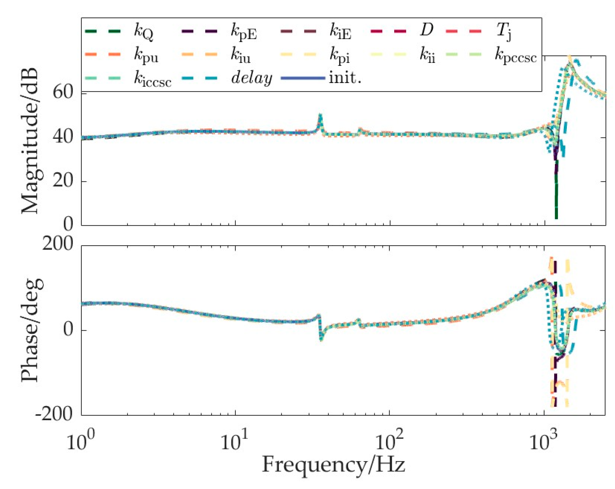
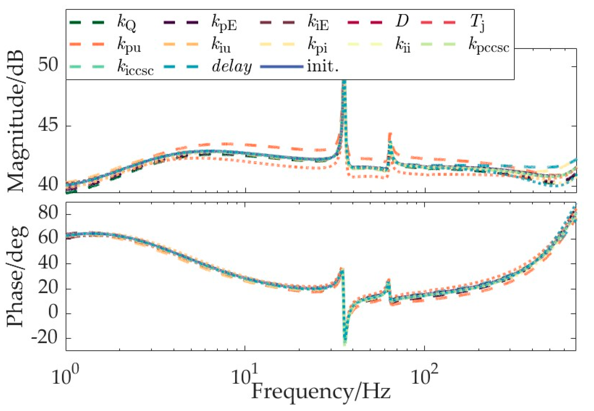
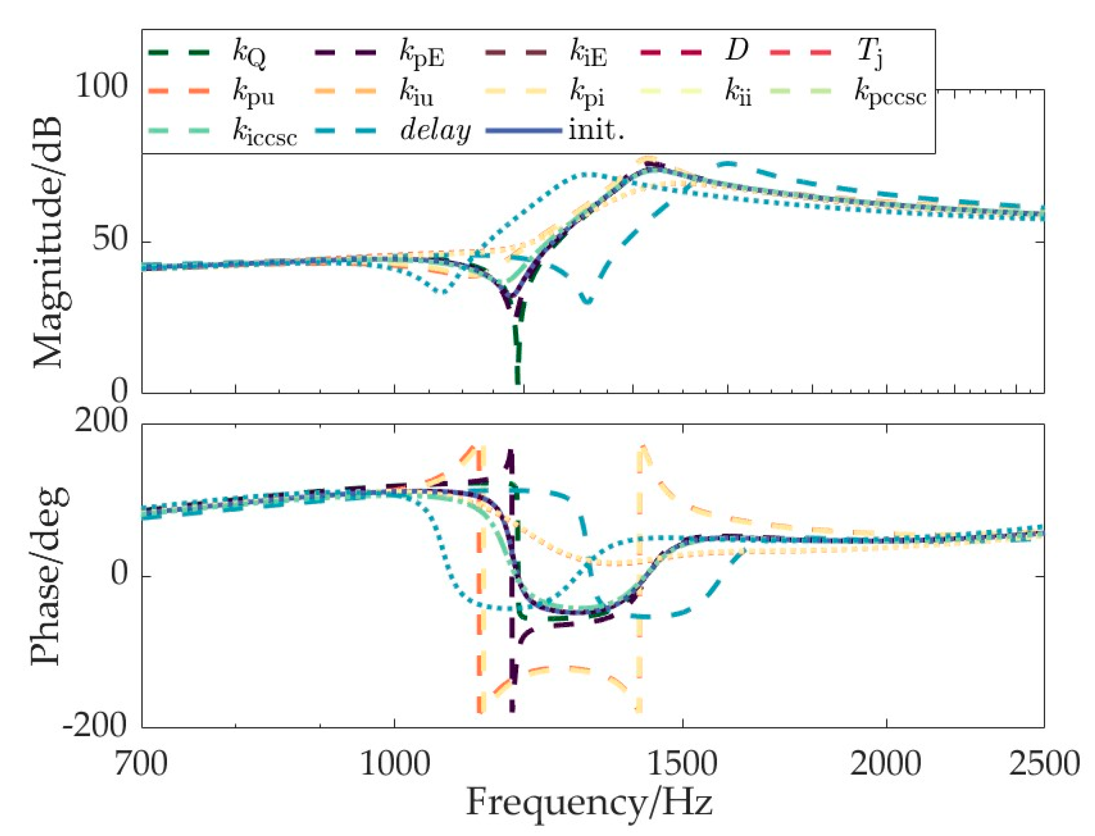
3.1. Analysis of Factors Affecting Wideband Impedance of MMC under Grid-Forming Control

For MMC employing grid-forming control, the control system parameters consist of parameters for virtual synchronous control, PI parameters for virtual excitation control, voltage control and current control, PI parameters for circulating current suppression control, and control system delay, totaling 12 parameters. For the parameters listed in Table A2, based on the wideband impedance model of grid-forming MMC established in Section 2.3, the impact of reducing each control parameter to 90% of its initial value and increasing it to 1.1 times its initial value on the impedance characteristics of grid-forming MMC is studied. Figure 7 illustrates the wideband impedance characteristics of MMC under different control parameters. (init. represents the impedance characteristics with the initial control parameters).

Based on the trend of impedance magnitude variation in Figure 7, to avoid the influence of differences in impedance magnitude on the study of influencing factors, the impedance characteristics of grid-forming MMC can be roughly divided into two frequency ranges:

Frequency range I (below 700 Hz): The impedance magnitude of the MMC is generally flat, with only one resonance peak; the phase angle ranges from 0° to 90°, indicating inductive positive damping. Additionally, there is a narrow capacitive positive damping frequency range near the resonance peak of the MMC.

Frequency range II (700–2500 Hz): Multiple resonance peaks exist in the impedance magnitude of the MMC within this frequency range; the phase angle fluctuates significantly, with both capacitive negative damping and inductive negative damping present.

Next, the key factors influencing the impedance characteristics of the grid-forming MMC are analyzed in different frequency ranges.

The wideband impedance characteristics of the grid-forming MMC under different control parameters in frequency range I are shown in Figure 8.

According to Figure 8, the main influencing factors on the impedance magnitude-frequency and phase-frequency characteristics in frequency range I are mainly the PI parameters of the voltage control. Above 100 Hz, the influence of control delay, current control proportional coefficient k_pi, and virtual excitation control proportional coefficient k_pE on the impedance gradually increases with frequency, becoming the main influencing factor around 700 Hz. Therefore, the key influencing factors on the wideband impedance characteristics of the positive-sequence small-signal MMC in frequency range I are voltage control, control delay, current control, and virtual excitation control. When there is resonance risk in this frequency range, the MMC damping level can be optimized by adjusting the parameters of the voltage control, current control, and virtual excitation.

The wideband impedance characteristics of the grid-forming MMC under different control parameters in the frequency range II are shown in Figure 9. According to Figure 9, the impedance characteristics of the MMC in frequency range II are mainly influenced by the proportional coefficient k_pu of the voltage control, the proportional coefficient k_pi of the current control, and the control delay. Therefore, the key influencing factors on the wideband impedance characteristics of the MMC in frequency range II are voltage control, current control, and control delay. When there is resonance risk in this frequency range, the MMC damping level can be optimized by adjusting the proportional coefficients of these two control loops.

3.2. Comparison of Influencing Factors for MMC under Two Control Modes

By employing the same approach as in Section 3.1 to analyze the impedance characteristics of MMC under grid-following control, the key influencing factors of impedance characteristics for the grid-following MMC are identified as the power control and the PLL below 30 Hz. Between 30 Hz and 100 Hz, both the power control, current control, and PLL significantly affect the impedance characteristics. Above 100 Hz, the crucial influencing factors are the current control proportional coefficient and the control delay.

The key influencing factors of grid-following and grid-forming MMC are summarized in

Table 2. Key influencing factors of grid-following and grid-forming MMC.

Frequency Range	Grid-Following MMC	Frequency Range	Grid-Forming MMC
Below 30 Hz	kpp, kppll	Below 700 Hz	kpu, kpi, kpE, delay
30–100 Hz	kpp, kip, kppll, kpi, kii
100–2500 Hz	kpi, delay	700–2500 Hz	kpu, kpi, delay

.

Then, the differences between grid-following and grid-forming MMC on the key influencing factors can be summarized as follows:

• From the perspective of the key influencing factors on impedance characteristics across different frequency bands: The influence of power control/voltage control is significant in the low-frequency range. In the high-frequency range, the effects of control delay and the proportional coefficient of current control are dominant. For grid-following MMC, there exists a mid-frequency band where the impact of PLL is significant. Conversely, for grid-forming MMC, the influence of virtual synchronous control parameters remains insignificant in terms of wideband impedance. Moreover, the virtual excitation control parameters of grid-forming MMC exhibit significant effects across different frequency bands;
• From the perspective of optimizing parameters to suppress oscillations: Under grid-following control, the influencing factors in each frequency band are relatively independent, with fewer factors affecting individual frequency bands, resulting in lower flexibility in parameter optimization. Under grid-forming control, oscillation risks only exist in relatively high-frequency bands, where there are more influencing factors. Therefore, there is more flexibility in parameter optimization.

4. Analysis and Simulation of Wideband Oscillation Risk in Grid-Forming MMC

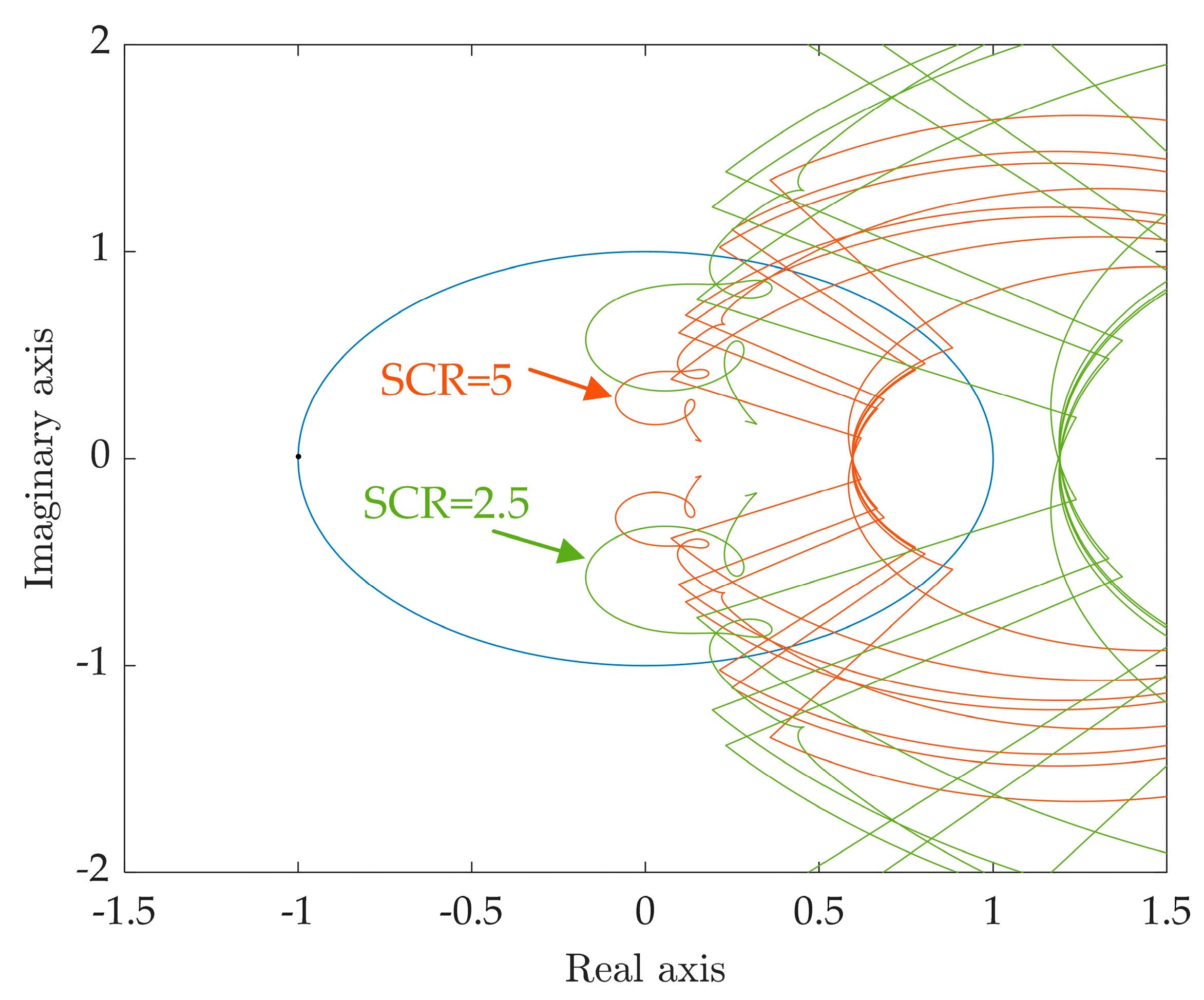
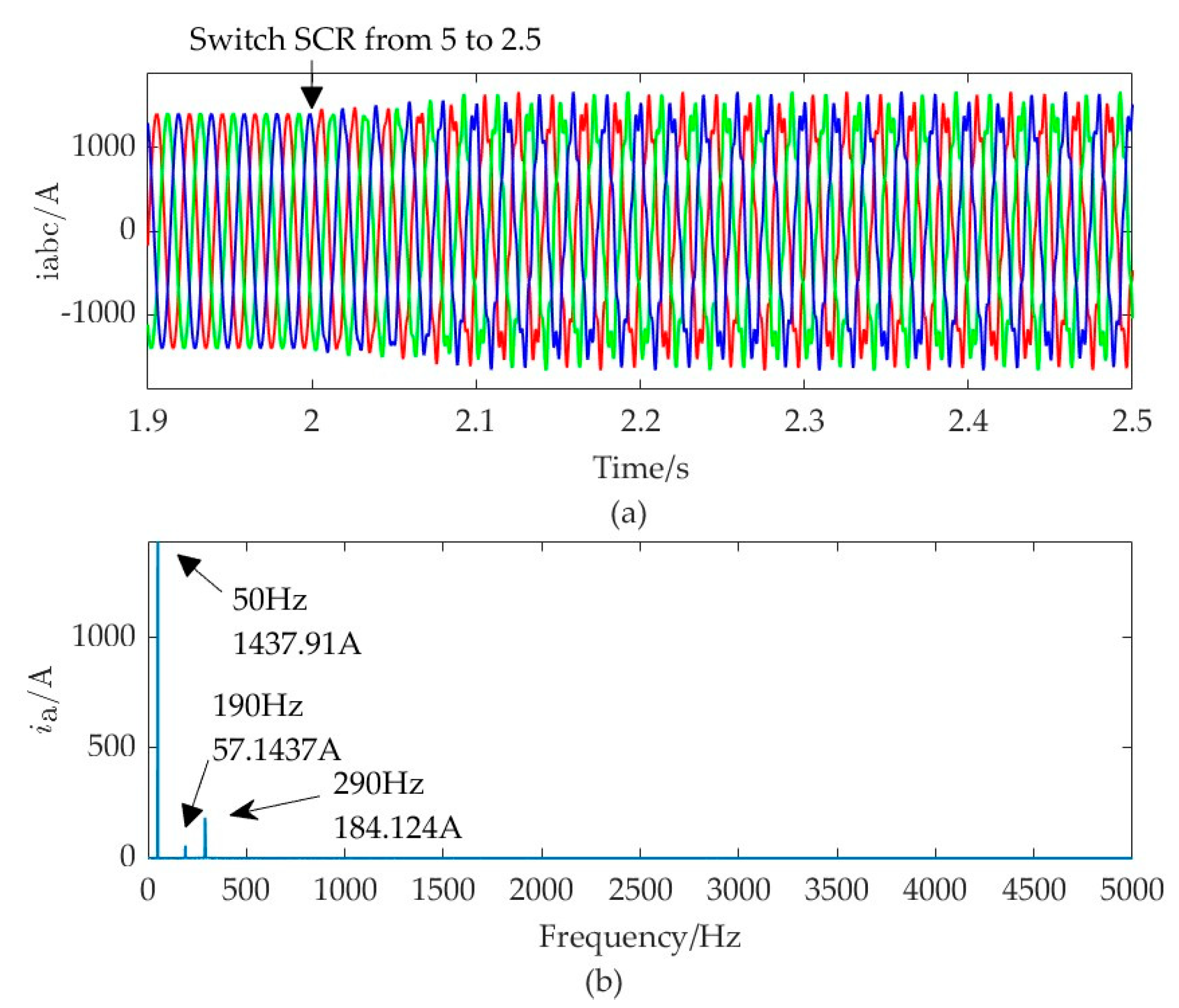
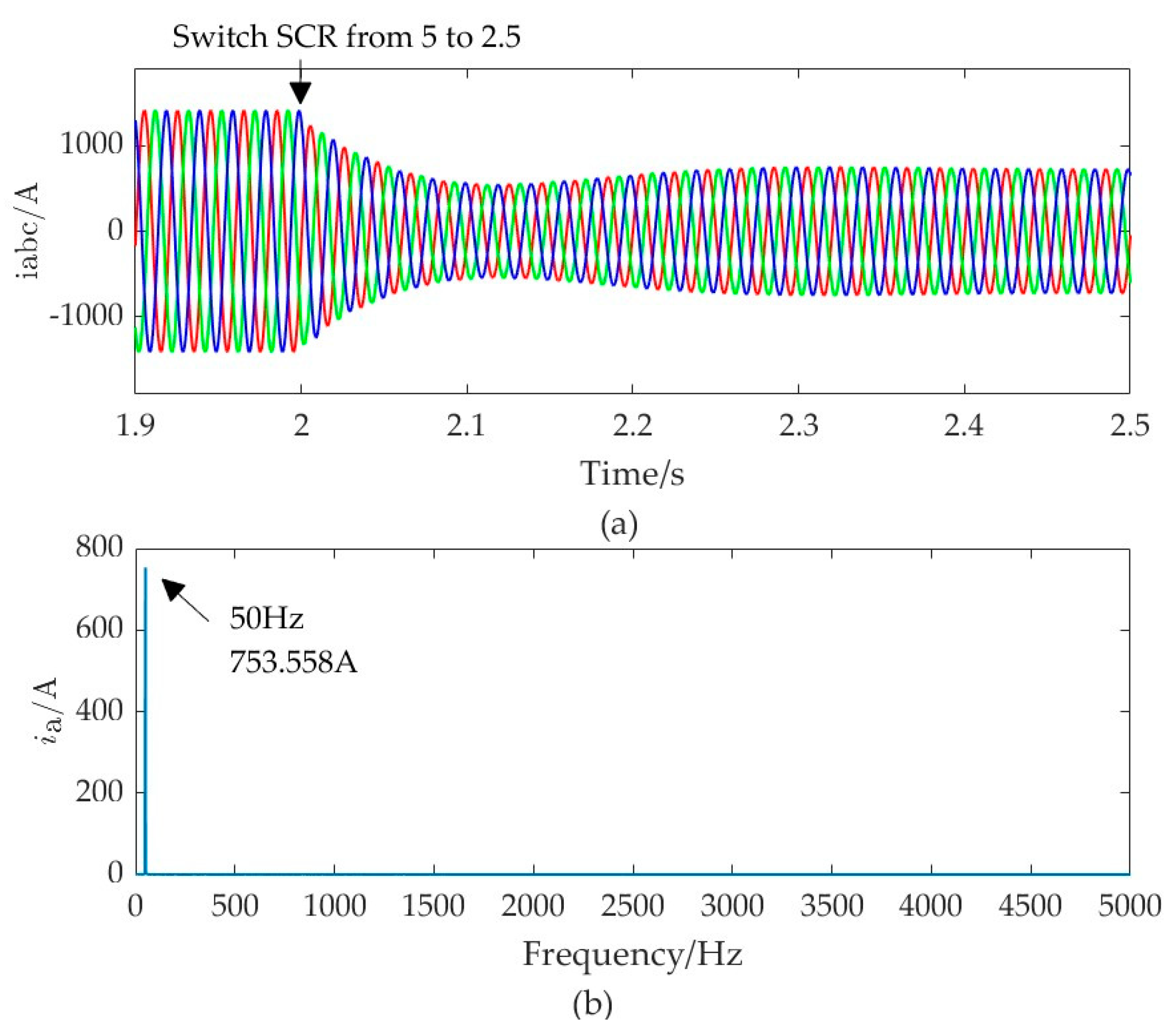
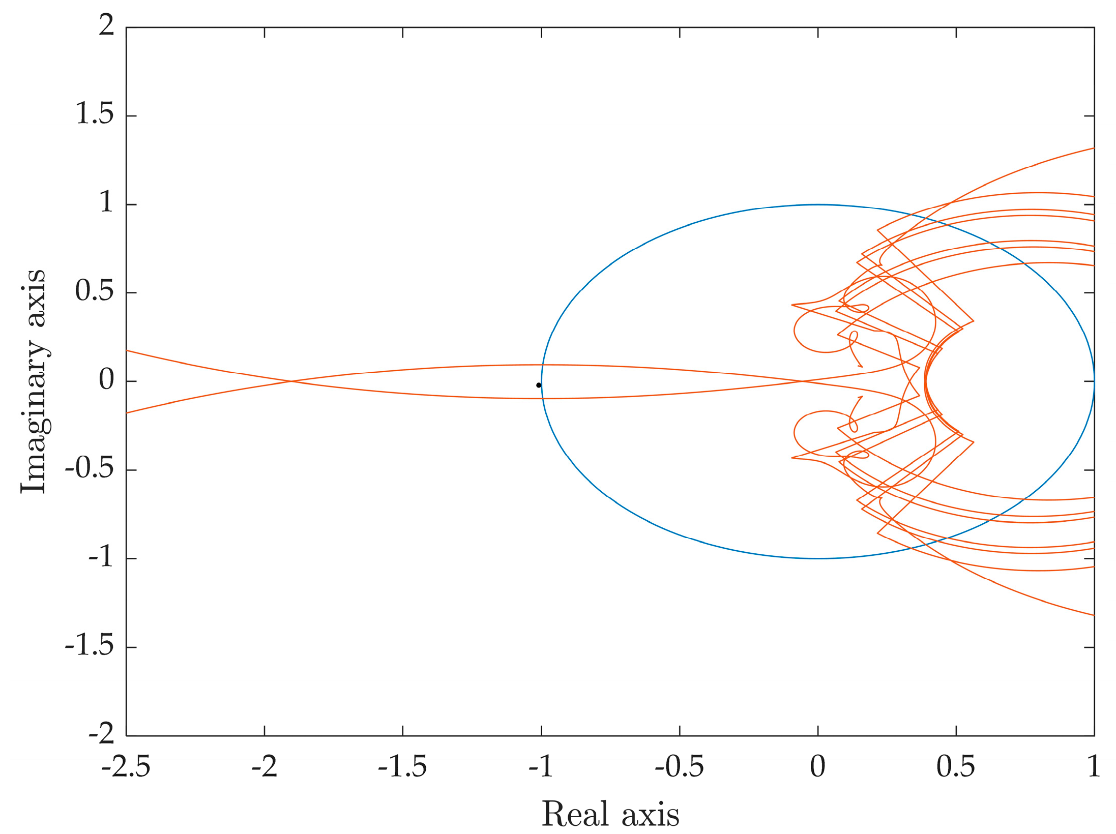
4.1. Oscillation Risk Caused by Grid Strength Variations

This section studies the oscillation risks of MMC-HVDC systems under changes in grid strength when MMC employs different control modes. The AC grid strength can be represented by the short circuit ratio (SCR). When the SCR changes from 5 to 2.5, indicating a weakening of the grid strength, the Nyquist plots of the MMC-HVDC systems under grid-following control and grid-forming control are shown in Figure 10 and Figure 11, respectively. As seen in Figure 10, when the AC grid strength weakens, the Nyquist plot of the system changes from not enclosing the (−1, 0) point to encircling it, indicating a transition from stability to instability of the system under grid-following control. At this point, the frequency at which the Nyquist curve crosses the unit circle is 242 Hz. According to the Nyquist criterion based on sequence impedance, after the grid switches from SCR = 5 to SCR = 2.5, the system will exhibit two oscillation frequency components in the time domain at 192 Hz and 292 Hz. Figure 11 shows that when the AC grid strength weakens, the Nyquist plot of the system under grid-forming control remains not encircling (−1, 0), indicating that the system remains stable under a wide range of variations in AC grid strength.

To validate the stability analysis conclusions depicted in Figure 10 and Figure 11, simulations are conducted. The initial state of the grid is set with SCR = 5, and at 2 s, the grid strength is switched to SCR = 2.5. The time-domain waveforms of the AC current for MMC under both grid-following and grid-forming control are observed, as shown in Figure 12 and Figure 13.

As for Figure 12, when MMC is under grid-following control, noticeable oscillatory components appear in the AC current waveform after the grid strength weakens. The spectrum of current reveals two distinct oscillatory components at 190 Hz and 290 Hz, closely matching the theoretically analyzed oscillation frequencies of 192 Hz and 292 Hz. This confirms the stability analysis conclusions depicted in Figure 10.

In contrast, as shown in Figure 13, when MMC is under grid-forming control, after the grid strength weakens, the spectrum of current shows only the fundamental frequency component. The AC current of the system transitions stably to a new steady-state operating point, thereby validating the stability analysis conclusions depicted in Figure 11.

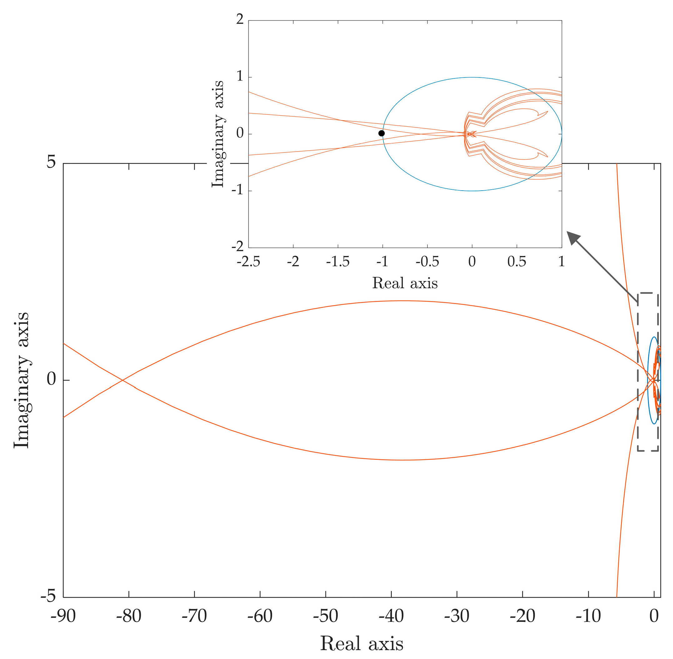
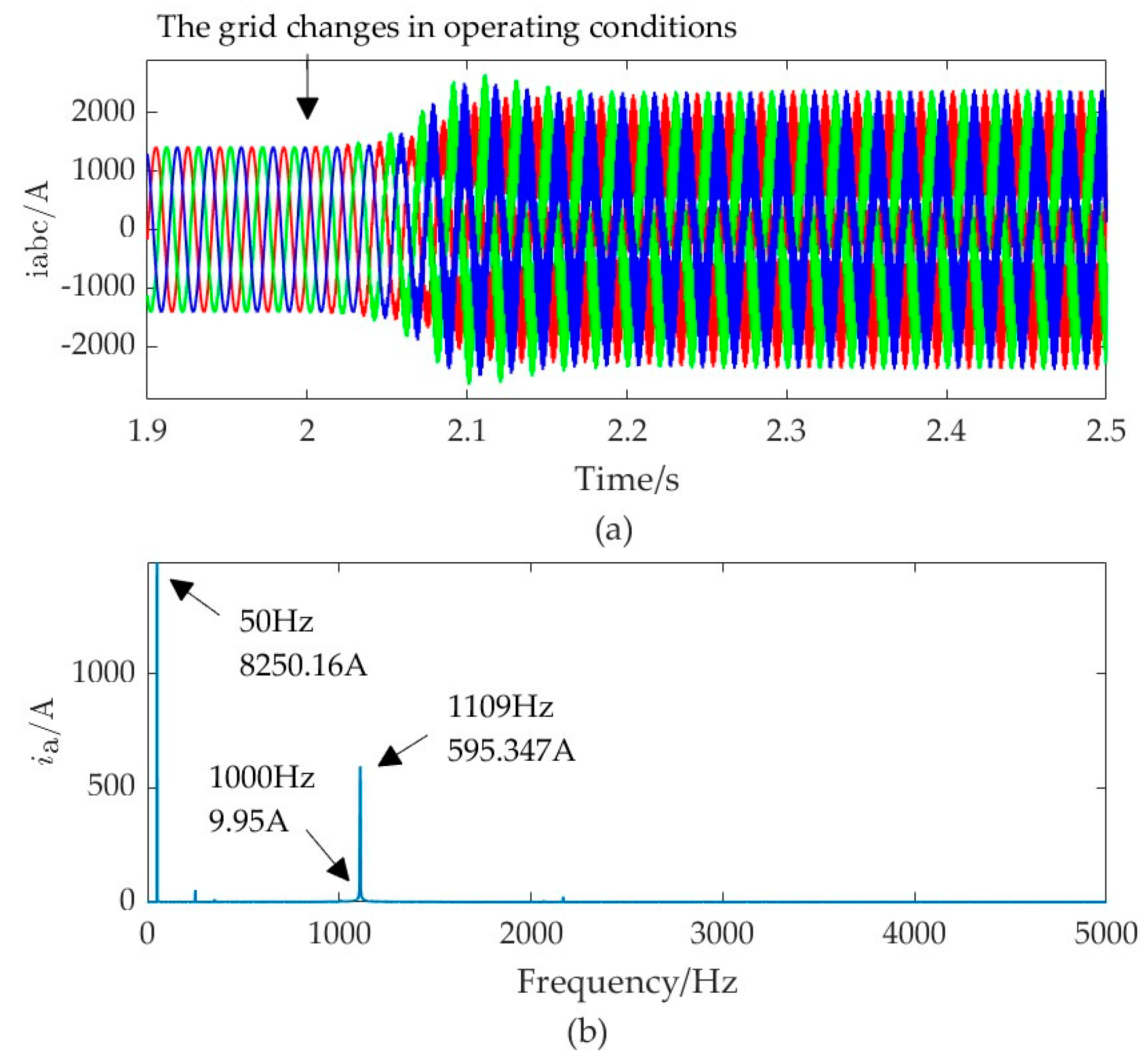
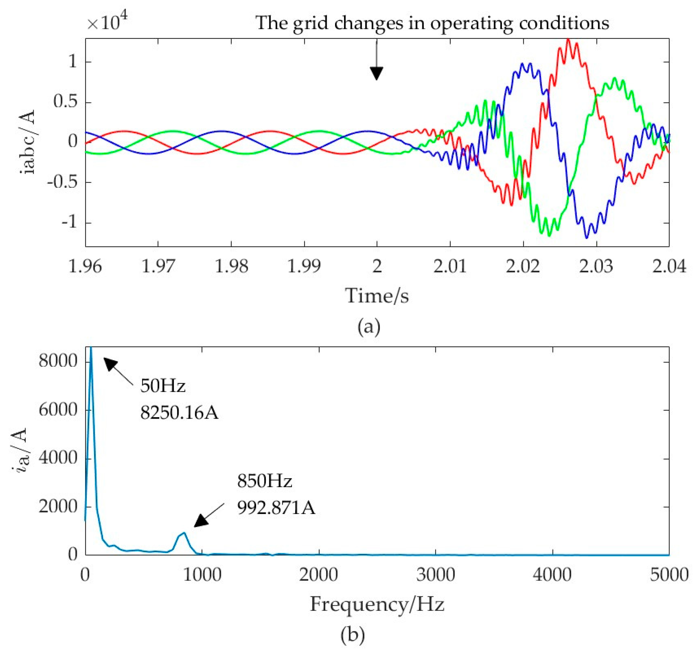
4.2. Oscillation Risk Caused by the Resonance Peak of Grid Impedance in a High-Frequency Range

This section studies the oscillation risk of MMC-HVDC systems under two control modes when there is a resonance peak in the high-frequency range of the AC grid impedance. The scenario of a resonance peak in the high-frequency range of the AC grid impedance is simulated in the simulation by modeling a series RLC resonance branch in parallel with the Thevenin equivalent impedance of the power source, with specific parameters as shown in Table A3.

When the resonance peak of the parallel resonance branch on the AC grid side is at 1200 Hz, the Nyquist plot of the system under grid-following control is shown in Figure 14. From the figure, it can be observed that the Nyquist plot of the system encircles the (−1, 0) point, indicating instability and high-frequency oscillations. According to Figure 14, when the MMC adopts the grid-following control mode, the Nyquist plot of the system crosses the unit circle at a corresponding frequency of 1071 Hz. According to the Nyquist criterion based on sequence impedance, the system will exhibit oscillation frequency components of 1021 Hz and 1121 Hz in the time domain.

When the resonance peak of the parallel resonance branch on the AC grid side is at 900 Hz, the Nyquist plot of the system under grid-forming control is shown in Figure 15. According to Figure 15, when the MMC adopts the grid-forming control, the Nyquist plot of the system crosses the unit circle at a corresponding frequency of 797 Hz. According to the Nyquist criterion based on sequence impedance, the system will exhibit oscillation frequency components of 747 Hz and 847 Hz in the time domain.

To verify the conclusions of the stability analysis presented in Figure 14 and Figure 15, simulations are conducted. In these simulations, the initial state of the grid equivalent impedance is modeled as an RL model, and at 2 s, a series RLC resonance branch is connected in parallel with the RL branch. The time-domain waveforms of the AC side currents of the system under both grid-following and grid-forming control are observed, as shown in Figure 16 and Figure 17.

From Figure 16, it can be observed that when the MMC adopts the grid-following control mode, significant oscillatory components appear in the AC side current after the grid impedance exhibits a resonance peak in the high-frequency range. The spectrum of current reveals the main oscillation component to be 1109 Hz, which matches the theoretical analysis result of 1121 Hz, confirming the stability analysis conclusion presented in Figure 14.

According to Figure 17, when the MMC adopts the grid-forming control mode, the AC side current of the system quickly diverges and exhibits significant oscillatory components after the grid impedance exhibits a resonance peak in the high-frequency range. The spectrum of current reveals the main oscillation component to be 850 Hz, matching the theoretical analysis result of 847 Hz, validating the stability analysis conclusion presented in Figure 15.

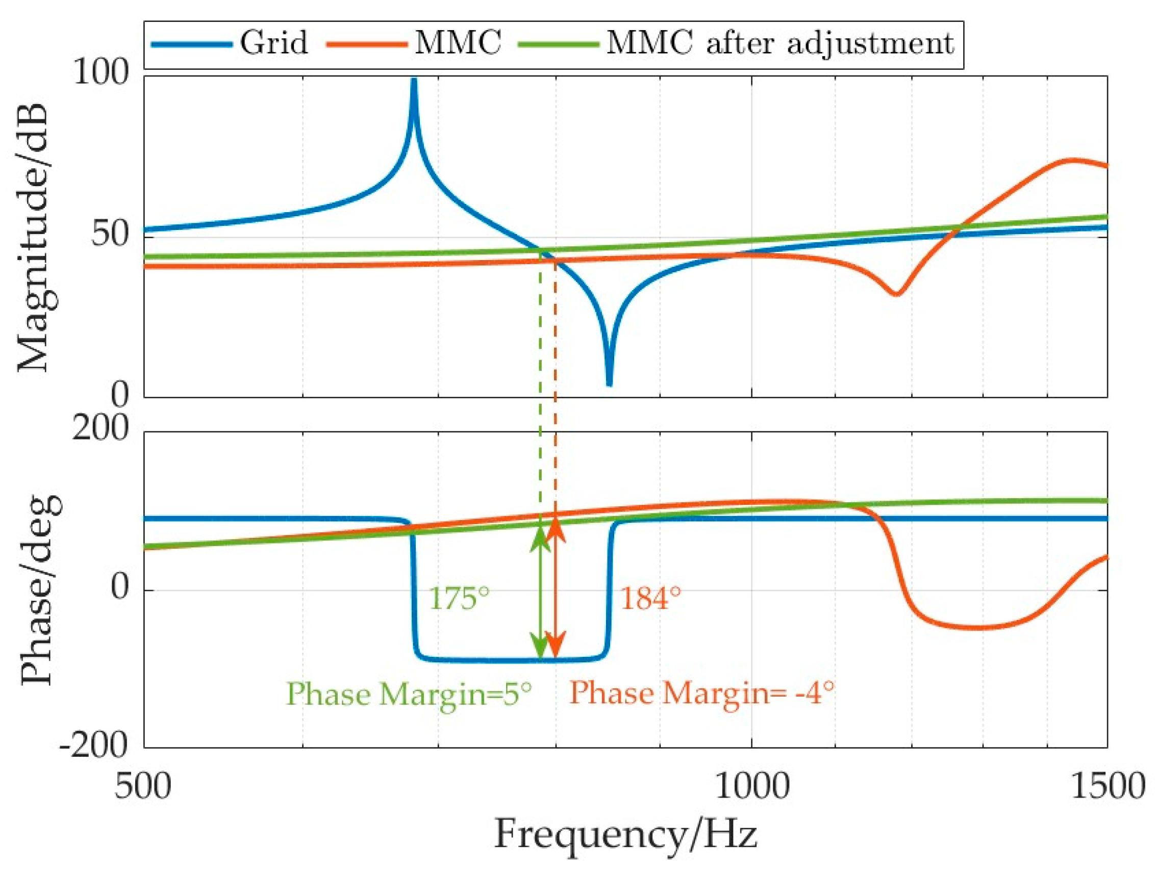
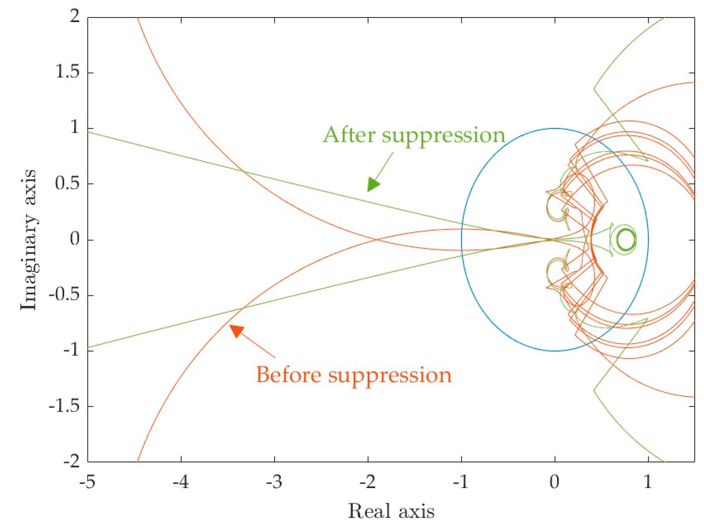
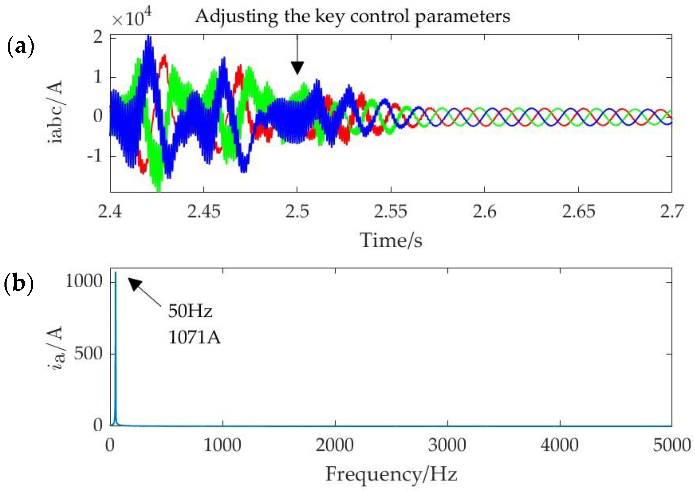
4.3. Wideband Oscillation Suppression Based on Key Control Parameter Adjustment

To verify the key control parameters of the impedance characteristics of gird-forming MMC in Section 3, this article suppresses the high-frequency oscillation risk by adjusting the key control parameters of grid-forming MMC.

According to the preceding discussion, the oscillation frequency is 850 Hz, falling within the frequency band II as outlined in Section 3.1. Consequently, the voltage control and current control parameters are the key control parameters influencing the impedance characteristics in this frequency band. Considering that the integration paths of PI controllers have little impact on the high-frequency characteristics of MMC, the suitable adjustable control parameters are the proportional coefficients of the voltage control and the current control.

The oscillation risk of the system is suppressed, and the phase margin of the system is increased by appropriately reducing k_pu and k_pi. The adjusted control parameters are shown in

Table 3. Control parameters before and after adjusting.

	Proportional Coefficient of the Voltage Control kpu	Proportional Coefficient of the Current Control kpi
Initial parameters	2.000	0.800
Adjusted parameters	1.960	0.384

.

After adjusting the control parameters, the Bode plot of the MMC and grid impedance characteristics is shown in Figure 18. It indicates that after adjusting the key control parameters, the phase margin at the oscillation risk frequency increases from −4° to 5°.

The Nyquist plot of the system after adjusting the key control parameters is shown in Figure 19. It can be observed that after adjustment, the Nyquist plot no longer encloses the (−1, 0) point, satisfying the stability criterion of the system.

In the simulation model, the key control parameters are implemented at 2.5 s. It is evident in Figure 20 that the oscillation phenomenon quickly disappears, and the current waveform rapidly returns to normal. In conclusion, the time-domain simulation results match well with the theoretical analysis.

5. Conclusions

This article establishes wideband impedance models for MMC under grid-forming and grid-following control. It compares and analyzes the differences in impedance characteristics under different control modes. The study also investigates the influencing factors and impedance characteristics of grid-forming MMC in various frequency ranges and analyzes the wideband oscillation risk of MMC. Furthermore, by adjusting the obtained key control parameters of MMC, this article effectively suppresses the oscillation risk discussed above. Finally, simulations are conducted to verify the accuracy of the wideband impedance model and the reliability of the stability analysis results. The main research conclusions of this article are summarized as follows;

• Compared to grid-following control, grid-forming control can confine the negative damping frequency band of MMC impedance characteristics from the wideband to the high-frequency band;
• Under grid-following control, the influencing factors in each frequency band are relatively independent, with fewer factors affecting individual frequency bands, resulting in lower flexibility in parameter optimization. Under grid-forming control, oscillation risks only exist in relatively high-frequency bands, where there are more influencing factors. Therefore, there is higher flexibility in parameter optimization;
• When the grid strength weakens, grid-following MMC faces instability risks, while grid-forming MMC can maintain stability. In instances where high-frequency resonance peaks exist in the impedance of the grid, both control modes of MMC may face instability risks;
• Adjusting the key control parameters of MMC can effectively suppress wideband oscillations.

References

1. Xu, J.; Liu, W.; Liu, S. Current state and development trends of power system converter grid-forming control technology. Power Syst. Technol. 2022, 46, 3586–3594. [Google Scholar]
2. Zhang, L.; Harnefors, L.; Nee, H.P. Power-synchronization control of grid-connected voltage-source converters. IEEE Trans. Power Syst. 2009, 25, 809–820. [Google Scholar] [CrossRef]
3. Ma, X.; Liu, Y.; Tian, J. Key technologies and challenges of grid-forming control for flexible DC transmission system. Autom. Electr. Power Syst. 2023, 47, 1–11. [Google Scholar]
4. Cao, Y.; Wang, W.; Li, Y. A virtual synchronous generator control strategy for VSC-MTDC systems. IEEE Trans. Energy Convers. 2017, 33, 750–761. [Google Scholar] [CrossRef]
5. Rocabert, J.; Luna, A.; Blaabjerg, F.; Rodriguez, P. Control of Power Converters in AC Microgrids. IEEE Trans. Power Electron. 2012, 27, 4734–4749. [Google Scholar]
6. Yu, J.; Wang, S.; Liu, Z. Accurate small-signal terminal characteristic model and SISO stability analysis approach for parallel grid-forming inverters in islanded microgrids. IEEE Trans. Power Electron. 2023, 38, 6597–6612. [Google Scholar] [CrossRef]
7. Ramezani, M.; Li, S.; Musavi, F. Seamless transition of synchronous inverters using synchronizing virtual torque and flux linkage. IEEE Trans. Ind. Electron. 2019, 67, 319–328. [Google Scholar] [CrossRef]
8. Zhan, C.; Wu, H.; Wang, X. An overview of stability studies of grid-forming voltage source converters. Proc. CSEE 2023, 43, 2339–2358. [Google Scholar]
9. Zhang, H.; Xiang, W.; Lin, W. Grid forming converters in renewable energy sources dominated power grid: Control strategy, stability, application, and challenges. J. Mod. Power Syst. Clean Energy 2021, 9, 1239–1256. [Google Scholar] [CrossRef]
10. Rosso, R.; Cassoli, J.; Buticchi, G. Robust stability analysis of LCL filter based synchronverter under different grid conditions. IEEE Trans. Power Electron. 2018, 34, 5842–5853. [Google Scholar] [CrossRef]
11. Chen, J.; Ren, Y.; Meng, Q. Sub-synchronous oscillation suppression strategy for grid-forming direct-drive permanent magnet synchronous generator with UDE supplementary damping branch. Trans. China Electrotech. Soc. 2023, 36, 1–16. [Google Scholar]
12. Wu, J.; Chen, X.; Zhang, D. Grid-connected stability analysis and improvement strategy for grid-forming energy storage system in new energy access scene. Proc. CSEE 2024, 44, 1–14. [Google Scholar]
13. Liu, J. Stability Mechanism and Power Oscillation Analysis of Power System with High-Penetration wind Power and Photovoltaic Generation. Ph.D. Thesis, Zhejiang University, Hangzhou, China, 2022. [Google Scholar]
14. Liu, P.; Xie, X.; Li, Y. Mechanism and characteristics of grid-forming control for improving sub/super synchronous oscillation stability of grid-following-based grid-connected converter. Power Syst. Technol. 2024, 48, 1–9. [Google Scholar]
15. Hu, Y.; Tian, Z.; Zha, X. Impedance stability analysis and promotion strategy of islanded microgrid dominated by grid-connected and grid-following converters. Autom. Electr. Power Syst. 2022, 46, 121–131. [Google Scholar]
16. Liu, Z.; Luo, J.; Liang, N. Analysis of influence of virtual synchronous control on sub-synchronous oscillation damping for grid-connected wind power system. Autom. Electr. Power Syst. 2023, 47, 135–147. [Google Scholar]
17. Wu, G. Passivity-Based High-Frequency Oscillation Mitigation Strategies for Three-Phase Grid-Forming Inverters. Master’s Thesis, Huazhong Institute of Scinence and Technology, Wuhan, China, 2022. [Google Scholar]
18. Zong, H.; Zhang, C.; Bao, Y. Frequency-domain modeling and synchronization perspective interaction mechanism of GFL-GFM converter system. J. Shanghai Jiaotong Univ. 2023, 37, 1–22. [Google Scholar]
19. Wu, W.; Chen, Y.; Zhou, L. Sequence impedance modeling and stability analysis for virtual synchronous generator connected to the weak grid. Proc. CSEE 2019, 39, 1560–1571. [Google Scholar]
20. Wu, W.; Zhou, L.; Chen, Y. Sequence-impedance-based stability comparison between vsgs and traditional grid-connected inverters. IEEE Trans. Power Electron. 2019, 34, 46–52. [Google Scholar] [CrossRef]
21. Huang, Y.; Ma, X.; Zhang, J. Study on the optimization of damping control strategy for grid-forming VSC-HVDC. Power Syst. Technol. 2023, 47, 21–29. [Google Scholar]
22. Zou, C.; Rao, H.; Xu, S. Analysis of resonance between a VSC-HVDC converter and the AC grid. IEEE Trans. Power Electron. 2018, 33, 10157–10168. [Google Scholar] [CrossRef]
23. Zhu, S. MMC Models Considering Harmonic Interaction and Their Application to Small-Signal Stability Analysis. Ph.D. Thesis, Wuhan University, Wuhan, China, 2021. [Google Scholar]
24. Yang, S.; Liu, K.; Qin, L. A broadband active damping method for high-frequency resonance suppression in mmc-hvdc system. Int. J. Electr. Power Energy Syst. 2023, 146, 108791. [Google Scholar] [CrossRef]
25. Pan, R.; Liu, D.; Liu, S. Stability comparison between grid-forming and grid-following based wind farms integrated mmc-hvdc. J. Mod. Power Syst. Clean Energy 2023, 11, 1341–1355. [Google Scholar] [CrossRef]
26. Zhu, S.; Qin, L.; Liu, K. Impedance modeling of modular multilevel converter in d-q and modified sequence domains. IEEE J. Emerg. Sel. Top. Power Electron. 2022, 10, 4361–4382. [Google Scholar] [CrossRef]
27. Zhu, S.; Liu, K.; Liao, X. Dq frame impedance modeling of modular multilevel converter and its application in high-frequency resonance analysis. IEEE Trans. Power Deliv. 2020, 36, 1517–1530. [Google Scholar] [CrossRef]
Figure 1. Schematic diagram of single-phase bridge arm in MMC.
Energies 17 02507 g001
Figure 2. Schematic diagram of typical grid-following control.
Energies 17 02507 g002
Figure 3. Schematic diagram of typical grid-forming control.
Energies 17 02507 g003
Figure 4. Verification of grid-following MMC AC-side impedance.
Energies 17 02507 g004
Figure 5. Verification of grid-forming MMC AC-side impedance.
Energies 17 02507 g005
Figure 6. Comparison of positive sequence impedance characteristics of two control modes of MMC.
Energies 17 02507 g006
Figure 7. Different control parameter effects on grid-forming MMC impedance characteristics.
Energies 17 02507 g007
Figure 8. Different control parameter effects on grid-forming MMC impedance characteristics within frequency range I.
Energies 17 02507 g008
Figure 9. Different control parameter effects on grid-forming MMC impedance characteristics within frequency range II.
Energies 17 02507 g009
Figure 10. Nyquist plot of the system under grid-following control with weakening grid strength.
Energies 17 02507 g010
Figure 11. Nyquist plot of the system under grid-forming control with weakening grid strength.
Energies 17 02507 g011
Figure 12. AC-side current under grid-following control with weakening grid strength: (a) Time-domain waveform of three-phase current; (b) FFT analysis results of phase-A current from 2.5 s to 4 s.
Energies 17 02507 g012
Figure 13. AC-side current under grid-forming control with weakening grid strength: (a) Time-domain waveform of three-phase current; (b) FFT analysis results of phase-A current from 2.5 s to 4 s.
Energies 17 02507 g013
Figure 14. Nyquist plot of the system under grid-following control with high-frequency resonance branch in the grid.
Energies 17 02507 g014
Figure 15. Nyquist plot of the system under grid-forming control with a high-frequency resonance branch in the grid.
Energies 17 02507 g015
Figure 16. AC-side current under grid-following control with the resonance peak of grid impedance in the high-frequency range: (a) Time-domain waveform of three-phase current; (b) FFT analysis results of phase-A current from 2.5 s to 4 s.
Energies 17 02507 g016
Figure 17. AC-side current under grid-forming control with the resonance peak of grid impedance in high-frequency range:(a) Time-domain waveform of three-phase current; (b) FFT analysis results of phase-A current from 2.01 s to 2.03 s.
Energies 17 02507 g017
Figure 18. Bode plot of impedance characteristics of the MMC and grid before and after adjusting the control parameters.
Energies 17 02507 g018
Figure 19. Nyquist plots of the system before and after adjusting the control parameters.
Energies 17 02507 g019
Figure 20. AC-side current under grid-forming control with high-frequency resonance peaks after adjusting the control parameters: (a) Time-domain waveform of three-phase currents. (b) FFT analysis results of phase-A current within the time interval from 2.6 s to 4 s.
Energies 17 02507 g020