2.1. Configuration of MMC
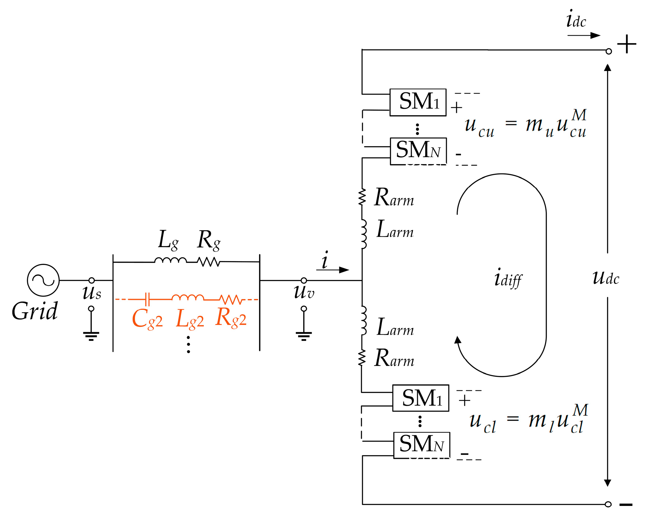
Figure 1 illustrates the diagram of the single-phase bridge arm structure of MMC.
uv represents the AC terminal voltage of MMC.
us represents the grid voltage.
i represents the AC-side current.
uCu and
uCl are the upper and lower pole voltages.
mu and
ml are the corresponding modulation signals.
and
are the equivalent voltages of the upper and lower bridge arms.
idiff represents the differential-mode current.
idc and
udc are the DC-side current and voltage.
Rarm and
Larm represent the equivalent resistance and equivalent inductance of the bridge arms, respectively.
Rg and
Lg represent the equivalent resistance and equivalent inductance of the grid, respectively. The impedance of the transformer can be integrated into the impedance of the power grid.
The average value model assumes consistent dynamic characteristics for all sub-modules and takes the sum of all capacitor voltages on each bridge arm as the system state variable. The average value model representing the dynamic behavior of a single-phase MMC is expressed as:
where
Carm represents the equivalent capacitance of the bridge arm, which can be calculated as
CSM/
N.
CSM represents the capacitance of each submodule and
N represents the number of submodules in a single bridge arm.
The average model of MMC is a nonlinear time-periodic (NTP) model, which is difficult to analyze directly. The linear time-invariant (LTI) model of MMC is established using the harmonic state-space (HSS) modeling method, followed by the derivation of the small-signal impedance model for MMC.
2.2. Harmonic State-Space Modeling Theory
The state equation of MMC shown in Equation (1) can be expressed in the following form of NTP model:
where
x,
u, and
y represent the state vector, input vector, and output vector, respectively, while
f and
g are nonlinear algebraic functions.
By employing the HSS modeling method, the time-domain model is transformed into the harmonic domain in the authors’ previous work [
26].
The model of the MMC can be expressed as:
where the state variable
, input variable
, and intermediate variable
. The expressions for the coefficient matrices in Equation (4) are provided in
Appendix A.
In the HSS model, the coefficient matrices can be represented as
AHx = Γ(
ATx)
,AHz = Γ(
ATz),
BH = Γ(
BT). Therefore, these matrices are represented by complex Fourier coefficients of different harmonic orders, which are expressed in terms of amplitude and phase angle rather than time-varying signals. For instance,
AHx1 and
AHx−1, the two elements of
AHx, are composed of the positive and negative sequence fundamental frequency components of
ATx, respectively. These Fourier coefficients can be obtained through simulation or calculated using the method described in ref. [
27]. Oscillation frequencies in current engineering applications are all below 2500 Hz. Within this frequency range, the inductance of reactors and the capacitance of capacitors can be considered constant. Therefore, the frequency-dependent effects of power electronic devices can be neglected in this article.
2.3. Broadband Impedance Model of Grid-Forming MMC
The open-loop impedance model of MMC serves as the basis for closed-loop impedance models under control. Therefore, this section illustrates the derivation process from the state equation to the open-loop impedance model by introducing the HSS modeling method.
In open-loop control conditions, the disturbance of the modulation signal is zero, hence ∆
z = 0. Then,
, the simplified time-domain LTP equation can be transformed from the time domain to the harmonic domain. By letting the output variable be the state variable, i.e.,
, the harmonic input-output relationship can be expressed as:
The expression for the harmonic transfer matrix
can be found in
Appendix A.
The definition of
Ypn11 is the MMCs sequence admittance when the third and higher harmonics are neglected. Clearly,
Ypn11 is a sub-matrix of
. Considering the dynamics of the
h-th higher harmonic, where the length of the column vectors
and
are 4 × (2h + 1) and 2 × (2h + 1), respectively, the fundamental frequency sequence admittance of the MMC is:
where
denotes the element of matrix
in the
i-th row and the
j-th column. When higher harmonics are considered in the HSS model, higher harmonic Fourier series coefficients need to be added to all harmonic transfer matrices using a similar modeling approach. Based on the fundamental frequency sequence admittance of the MMC, the open-loop sequence impedance of the MMC can be obtained by matrix inversion.
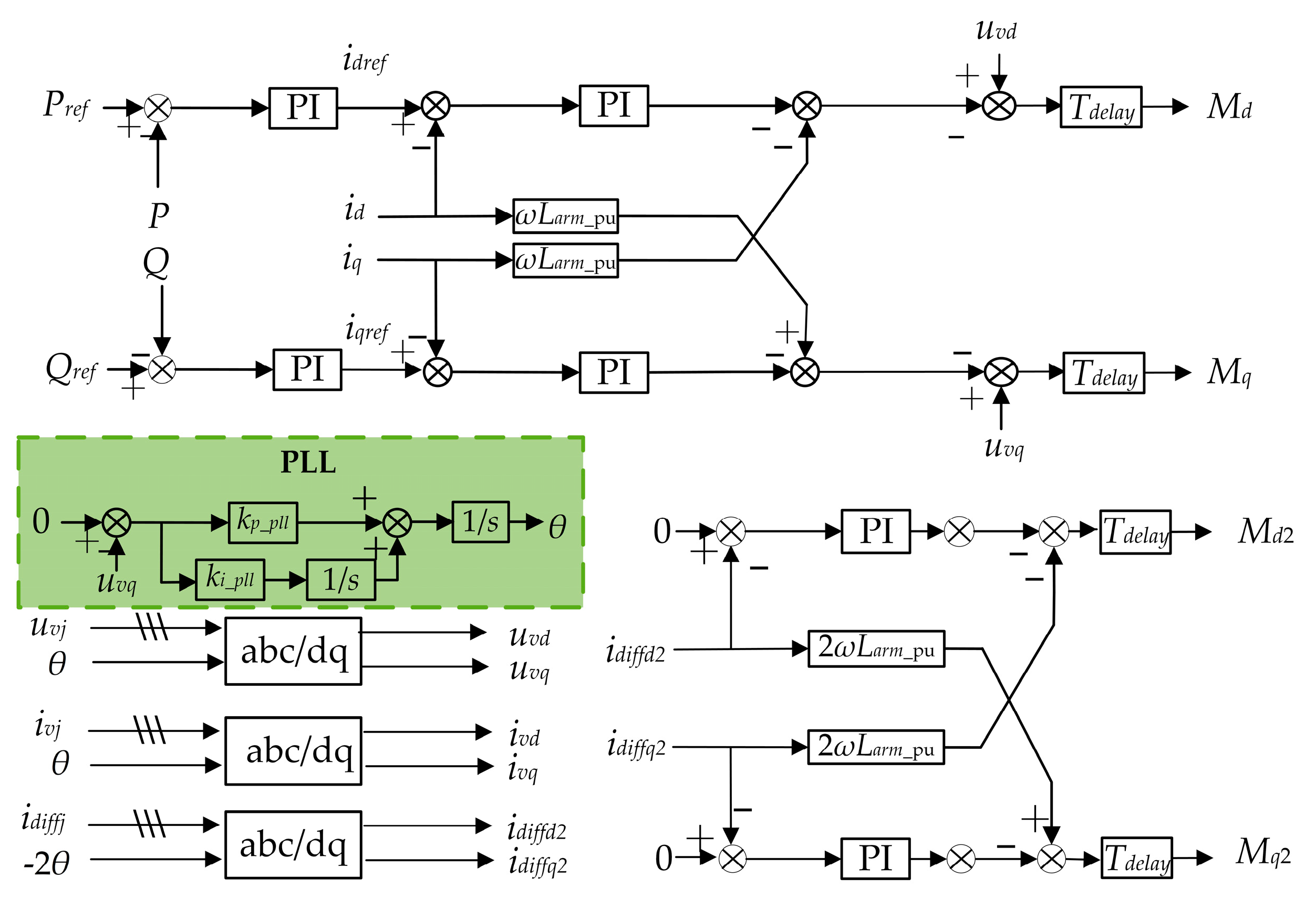
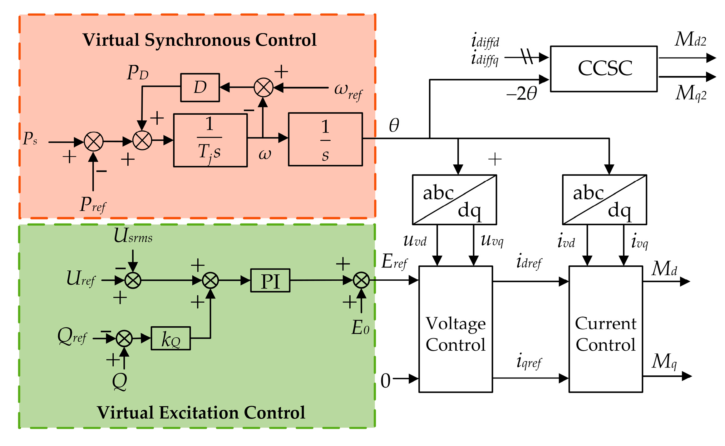
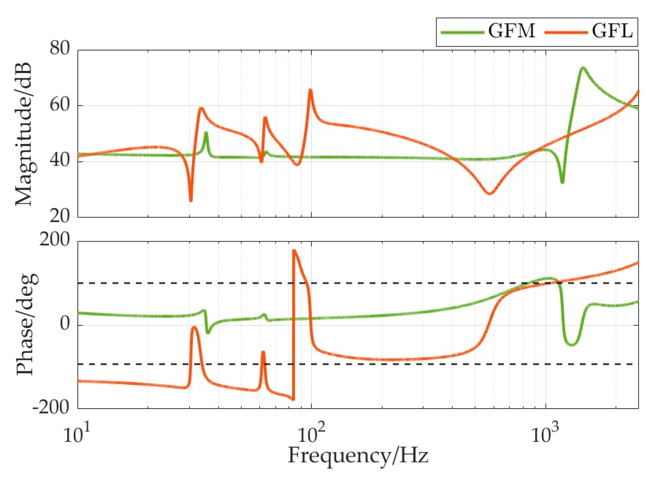
To study the oscillation risk of the MMC-HVDC system under grid-forming control and compare it with grid-following control, this article selects conventional dual-loop control with constant PQ as the outer loop, provided by a phase-locked loop to supply phase, as a typical grid-following control method. For the grid-forming control method, it selects virtual synchronous control with virtual excitation control (internal potential amplitude calculation) providing voltage control’s preference value and virtual rotor motion equations (virtual angle generation) providing phase. The control block diagrams for both control modes are shown in
Figure 2 and
Figure 3, respectively.
Due to the consistency of the current control, circulating current suppression control (CCSC), and modulation section under both control modes, this article will briefly introduce the basic method of closed-loop impedance modeling and the modeling process of obtaining phase under grid-forming control. In the following derivation, only textual explanations will be provided for certain matrices in the equations. The specific expressions can be found in the author’s previous work [
26].
When the controller is added, Δ
z ≠ 0, it is necessary to incorporate the controller dynamics into the system dynamic equations. For the convenience of implementing the impedance model in computer programming, the HSS model of the MMC is divided into four parts:
The first equation in (7) represents the dynamics of the electrical system. The intermediate variables
are the modulation signals for the upper and lower bridge arms. The second equation in (7) represents the transformation of the modulation signals.
and
represent the modulation signals outputted by the main control and CCSC, respectively. Based on the relationship between the modulation signals of the upper and lower bridge arms and the controller modulation signals, the expressions for the constant matrices
CHm1 and
CHm2 can be obtained [
23]. And
can be calculated from
and
. The third and fourth equations in (7) represent the dynamics of the main controller and CCSC, respectively. Therefore, the specific expressions of
DH1,
EH1,
DH2, and
EH2 depend on the control method used by the MMC. After obtaining the expressions of the transfer function matrices in Equation (7), the transfer function matrix from
to
can be written as:
Once the expressions for are obtained, the derivation process for the open-loop impedance is consistent with the process outlined in Equation (6), yielding the fundamental frequency sequence admittance and impedance of the MMC.
Next, this paper derives the expressions for DH1, EH1, DH2, and EH2 under grid-forming control, obtaining the closed-loop broadband impedance model of grid-forming MMC.
The key disparity distinguishing the control system of the MMC under grid-forming control from that under grid-following control lies in the provision of phase information by the virtual rotor motion equation. Therefore, the crucial step in establishing the wideband impedance model of the grid-forming MMC is to express the HSS form of the virtual angle generation.
To illustrate the process of obtaining the phase through virtual synchronous control, the virtual rotor dynamics equation under grid-forming control can be written as:
where
Tj represents the inertia time constant,
D stands for the damping coefficient, and
ω denotes the virtual angular velocity used in control.
Ps represents the output active power and
Pref represents the reference value of active power.
Linearizing Equation (9) and transforming it into the frequency domain, its HSS form can be expressed as:
where,
The expression for
can be expressed as:
According to the expression of
, we can derive the coordinate transformation equations for each variable, and subsequently deduce the HSS forms of virtual excitation control, voltage control, and current control. The detailed derivation process is provided in
Appendix C.
Finally, we can obtain the expressions for
DH1 and
EH1:
Since the dynamics of
depend on the
and
in
Appendix C, an additional coefficient matrix
needs to be added to the HSS representation of the current loop controller, denoted as
FH2. By substituting the coordinate transformation equations of each variable into the expression for the CCSC dynamics, the expressions for
DH2,
EH2, and
FH2 can be furtherly obtained:
The transfer function matrix from
to
can be represented as:
Based on the expression for
, the fundamental frequency sequence admittance and sequence impedance of MMC under grid-forming control mode can be obtained using Equation (6). The abbreviations table explaining the symbols appearing in the modeling process of this article are as shown in
Table A1.


