Grid Model of Energy Consumption Using Random Forest by Integrating Data on the Nighttime Light, Population, and Urban Impervious Surface (2000–2020) in the Guangdong–Hong Kong–Macau Greater Bay Area

Abstract

Energy consumption is an important indicator for measuring economic development and is closely related to the atmospheric environment. As a demonstration zone for China’s high-quality development, the Guangdong–Hong Kong–Macao Greater Bay Area imposes higher requirements on ecological environment and sustainable development. Therefore, accurate data on energy consumption is crucial for high-quality green development. However, the statistical data on local energy consumption in China is insufficient, and the lack of data is severe, which hinders the analysis of energy consumption at the metropolitan level and the precise implementation of energy policies. Nighttime light data have been widely used in the inversion of energy consumption, but they can only reflect socio-economic activities at night with certain limitations. In this study, a random forest model was developed to estimate metropolitan-level energy consumption in the Guangdong–Hong Kong–Macao Greater Bay Area from 2000 to 2020 based on nighttime light data, population data, and urban impervious surface data. The estimation results show that our model shows good performance with an R² greater than 0.9783 and MAPE less than 9%. A long time series dataset from 2000 to 2020 on energy consumption distribution at a resolution of 500 m in the Guangdong–Hong Kong–Macao Greater Bay Area was built using our model with a top-down weight allocation method. The spatial and temporal dynamics of energy consumption in the Greater Bay Area were assessed at both the metropolitan and grid levels. The results show a significant increase in energy consumption in the Greater Bay Area with a clear clustering, and approximately 90% of energy consumption is concentrated in 22% of the area. This study established an energy consumption estimation model that comprehensively considers population, urban distribution, and nighttime light data, which effectively solves the problem of missing statistical data and accurately reflects the spatial distribution of energy consumption of the whole Bay Area. This study provides a reference for spatial pattern analysis and refined urban management and energy allocation for regions lacking statistical data on energy consumption.

1. Introduction

Energy consumption is an important indicator that reflects social production activities and the economic development of a region [1,2,3]. It also serves as a crucial basis for assessing the ecological environment and carbon emissions [4,5,6], especially in light of the current dual carbon targets in China (achieving “peak carbon” by 2030 and “carbon neutrality” by 2060). An accurate understanding of the spatiotemporal development patterns of energy consumption is of great importance for assessing energy security, formulating science-based energy development policies, and achieving green and low-carbon development. The data on energy consumption in China mainly comes from the “China Energy Statistical Yearbook” and local “Statistical Yearbooks”, especially at the national and provincial levels. Little statistical data are available at the municipal level. For example, only 53.5% of the energy consumption statistics for cities in Guangdong Province are available for the period 2000 to 2020. Energy consumption data at the county level is almost empty. The severe lack of data has meant that current research on energy consumption focuses mainly on the national and provincial level [7,8,9], limiting micro-level studies of energy consumption within cities. This limitation also prevents the differences among cities in energy consumption from being taken into account and is an obstacle to the rational formulation of energy consumption policy.

Nighttime light data provide valuable insights into human activity patterns and urban development dynamics. These data capture the intensity and spatial distribution of artificial light emissions, offering an objective and real-time depiction of social dynamics within urban areas. Researchers have extensively utilized nighttime light data to estimate various socio-economic parameters, including urbanization levels, economic activity, and energy consumption [10,11,12,13]. Regarding the use of nightlight data to estimate energy consumption, pioneering work was conducted in 1980 by the American scientist Welch, who investigated the relationship between the area of nighttime light from DMSP/OLS data and energy consumption within the administrative boundaries of the United States. He proved that it is possible to estimate energy consumption from DMSP/OLS data at a national or regional level [14]. Since then, numerous researchers have conducted studies on energy consumption based on nighttime light data. Amaral et al. estimated energy consumption in the Brazilian Amazon basin using nocturnal DMSP nighttime satellite data and demonstrated a linear correlation between light area and electricity consumption, confirming the feasibility of assessing human activities in the Brazilian Amazon region [15]. Letu et al. investigated the correlation between nighttime DMSP/OLS light intensity and energy consumption in 12 Asian countries and found that polynomial (cubic) regression provided a better result for estimating energy consumption [16]. Wu et al. recovered the spatiotemporal variation in energy consumption in prefecture-level cities in 30 Chinese provinces from 1995 to 2009 based on the linear relationship between total nighttime light values and provincial energy statistics data [17]. Bai integrated DMSP/OLS remote sensing data with MODIS Normalized Difference Vegetation Index (NDVI) data to simulate total energy consumption at the prefecture level in China from 2000 to 2010 [18]. Xie and Weng constructed a panel model with a fixed time effect between nighttime light and total energy consumption and discovered a significant positive correlation between the two at global and regional scales [13]. Xiao et al. established a geographically and temporally weighted regression model between nighttime light and per capita energy consumption and energy consumption per unit area by simulating energy consumption in different provinces of China from 2000 to 2013. They then demonstrated the feasibility of rapid estimation of energy consumption in provinces of China using nighttime light data [19]. Tian estimated energy consumption in pre-stage cities in China using a panel model based on provincial nighttime lighting totals and energy consumption statistics and confirmed that the panel model was more reliable than the quadratic polynomial [20]. These studies have shown a linear correlation between global DMSP/OLS nighttime light data and energy consumption at the global, national, provincial, and city levels, confirming the feasibility of utilizing nighttime light data for estimating energy consumption. However, the exclusive use of nighttime light data also has its limitations, especially when it comes to mapping energy consumption with comprehensive socio-economic dynamics. To address this limitation, researchers often integrate complementary datasets such as population demographics, urban characteristics, and points of interest. Population demographic data, for example, provide insights into the demographic composition of areas, allowing for a more nuanced analysis of socio-economic trends [21,22]. Urban characteristics data, including land use patterns and infrastructure development, offer additional context for interpreting nighttime light data [23,24]. Points of interest data, such as the location of commercial establishments and cultural landmarks, contribute to a more holistic understanding of urban dynamics [25]. By integrating multiple datasets, researchers can enhance the robustness and accuracy of socio-economic estimations derived from nighttime light data, enabling more informed decision-making and policy formulation in various fields, including urban planning, environmental management, and disaster response.

The Guangdong–Hong Kong–Macao Greater Bay Area serves as an important gateway and spatial platform for China’s opening to the outside world. It plays an increasingly important role in leading the development trends of our times and driving global changes in production and lifestyle [26]. To achieve green, low-carbon, and sustainable development, it is essential to gain a detailed understanding of the spatial and temporal patterns of energy consumption within the Greater Bay Area urban cluster and the regional differences. However, the Guangdong–Hong Kong–Macao Greater Bay Area, as an urban agglomeration, has a significant lack of energy consumption statistics, which cannot support high-precision spatial–temporal analysis of energy consumption. At the same time, the current high-precision inversion of energy consumption is mainly based on a single source of nighttime light data, which does not fully reflect the actual situation of energy consumption. In this study, energy consumption is inverted and predicted based on nighttime light data, population distribution, and urban impervious surface data, which are all important factors influencing energy consumption. The brightness of nighttime light data shows a remarkable positive correlation with electricity consumption, reflecting the level of energy use in urban areas. The population distribution data provides information on the spatial distribution of energy demand, as densely populated regions tend to have higher energy consumption. In addition, the impervious surface data indirectly indicate the degree of urbanization, including building density and the development of the transport network. By integrating these three datasets, we can create an effective model to invert and predict urban energy consumption.

Based on the above analysis, the research objectives of this paper are as follows: (1) Analyze the spatiotemporal patterns of energy consumption in the Guangdong–Hong Kong–Macao Greater Bay Area. By utilizing the random forest algorithm and integrating multiple data sources including nighttime light data, population data, and urban impervious surface data, the aim is to elucidate the spatiotemporal patterns of energy consumption in the Greater Bay Area. (2) Fill the gap in city-level energy consumption data from 2000 to 2020 in the Guangdong–Hong Kong–Macao Greater Bay Area, which will provide a scientific basis for energy planning and environmental policy formulation in the region, promoting green, low-carbon, and sustainable development. (3) Provide a replicable method for energy consumption analysis. By developing the proposed methodology, a dataset of energy consumption in the Greater Bay Area with spatiotemporal characteristics at a resolution of 500 m is generated. This methodological framework can be widely applied to energy consumption studies at the city and county levels, serving as a valuable reference for regions lacking comprehensive energy statistics.

2. Materials and Methods

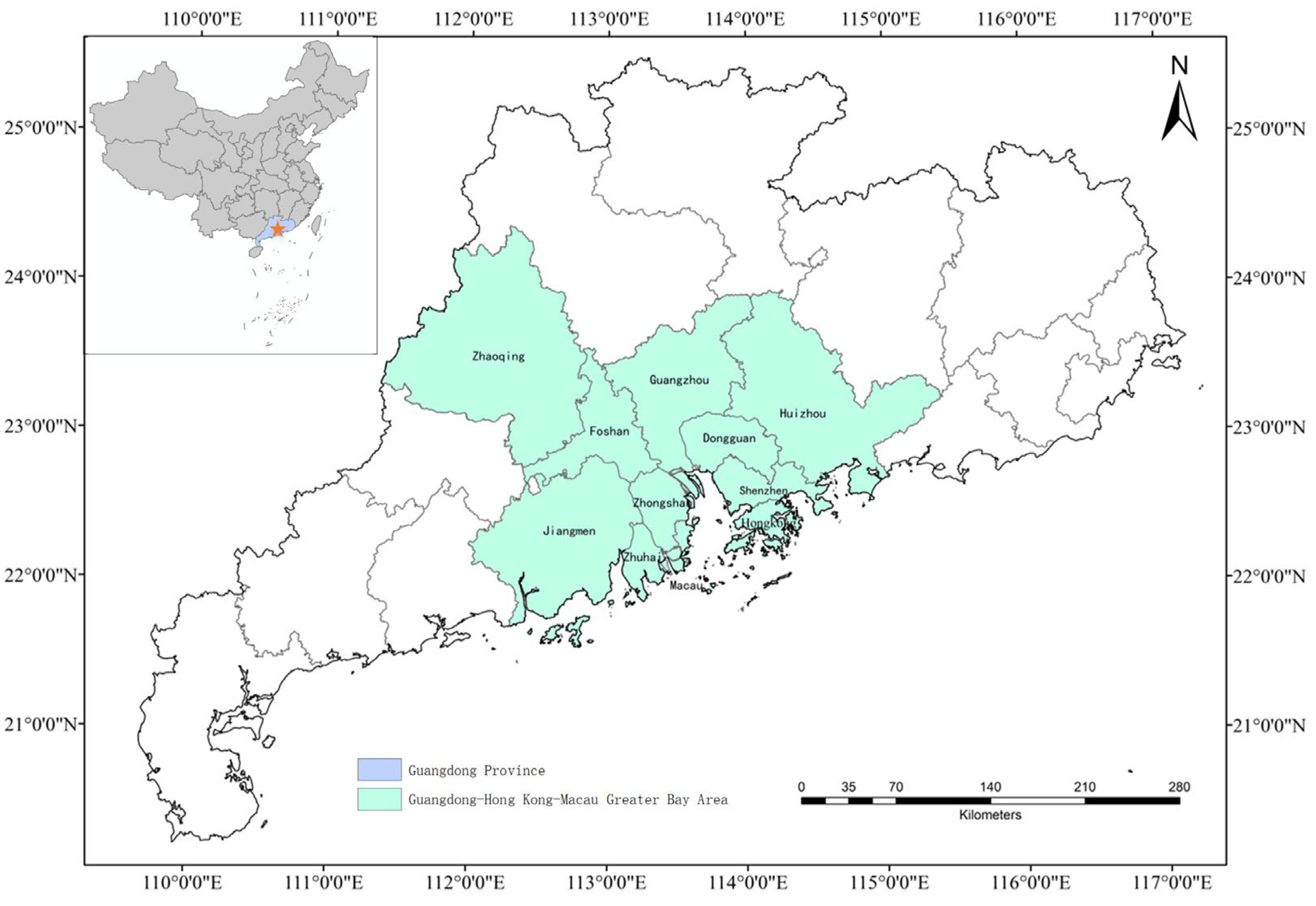
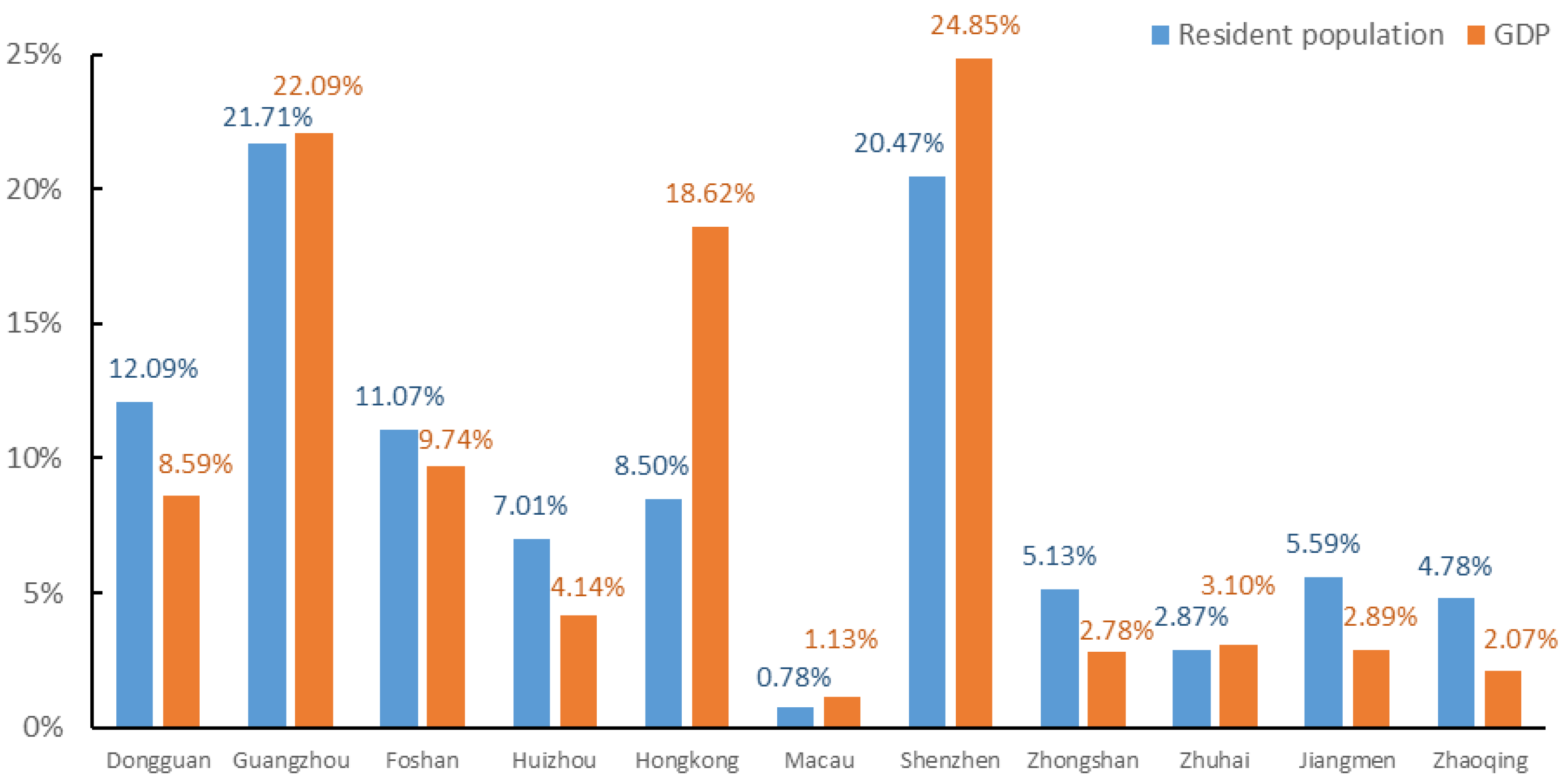
2.1. Study Area

The Guangdong–Hong Kong–Macao Greater Bay Area is an urban agglomeration consisting of the two special administrative regions of Hong Kong and Macao and nine cities in Guangdong Province, including Guangzhou, Shenzhen, Zhuhai, Foshan, Zhongshan, Dongguan, Zhaoqing, Jiangmen, and Huizhou (Figure 1). It is a key spatial unit in China’s efforts to create a world-class urban agglomeration and participate in global competition. It is comparable to the four major bay areas in the world, including the New York Bay Area and the San Francisco Bay Area in the United States and the Tokyo Bay Area in Japan. The total area of this region is 56,000 square kilometers, with a population of over 86 million in 2022. The total GDP exceeds CNY 13 trillion, making it one of the most open and economically dynamic regions in China. In the Guangdong–Hong Kong–Macao Greater Bay Area, Shenzhen, Guangzhou, and Hong Kong are the main core regions, accounting for 65.55% of the total regional GDP and 50.67% of the region’s total population (Figure 2). Over the past two decades, the GDP of the Greater Bay Area has experienced significant growth, rising from CNY 2.34 trillion in 2000 to CNY 13.04 trillion in 2022. This significant economic expansion has led to a substantial increase in energy consumption. As the rapid economic development in the Greater Bay Area continues, total energy consumption is expected to continue to rise. Currently, the structure of energy consumption in the Greater Bay Area is dominated by traditional energy sources such as coal and oil. However, as renewable energy technologies continue to advance, the region is gradually achieving a more diversified energy consumption structure, with the share of renewables in total energy consumption steadily increasing.

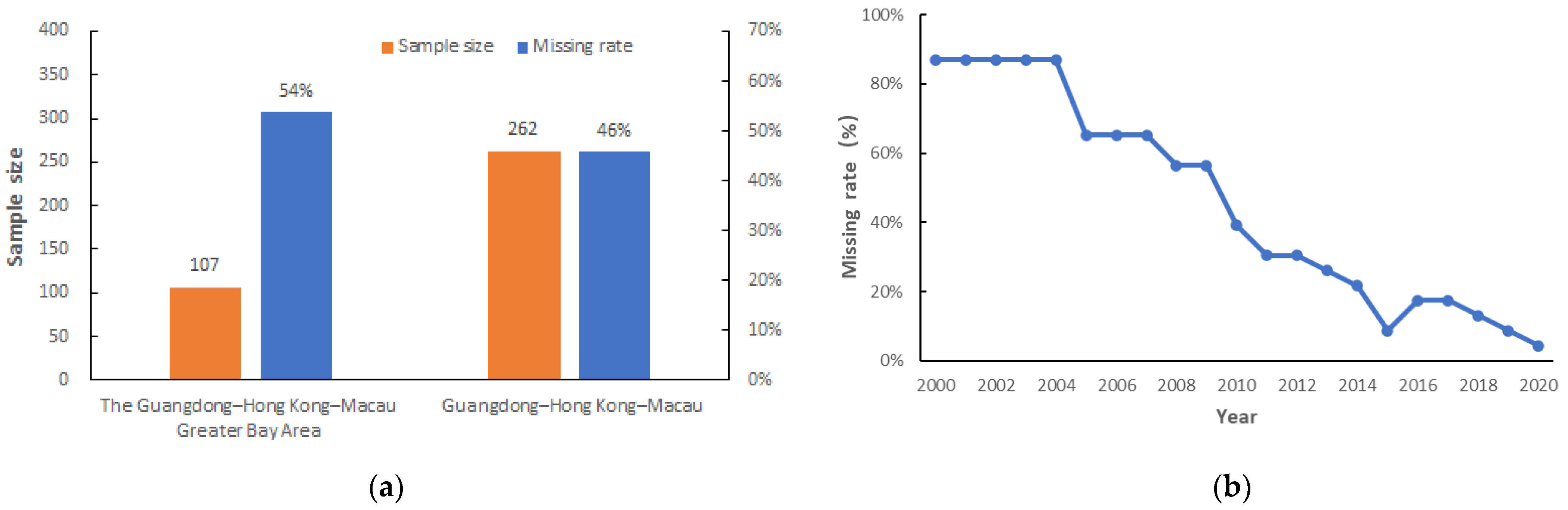
2.2. Data Sources

The nighttime light data came from the global 500-metre resolution dataset of “NPP-VIIRS-like” nighttime light data. This dataset was jointly researched and created by a team led by Professor Yu Baihang from East China Normal University, Associate Researcher Chen Zuozhi from Fuzhou University in China, and Associate Professor Shi Kaifang from Southwest University in China [27]. The team introduced a cross-sensor method for correcting nighttime light data based on autoencoders. They modified the autoencoder by using EANTLI (Enhanced and Corrected Defense Meteorological Satellite Program Operational Linescan System Imagery) data from 2013 as input and validated the output data with composite NPP-VIIRS (Visible Infrared Imaging Radiometer Suite on Suomi National Polar-orbiting Partnership) annual synthetic nighttime light data for the same year. After iterative training, the model was successively fed with EANTLI data from 2000 to 2012 to obtain corresponding “NPP-VIIRS-like” data for each year. This dataset has parameter attributes that match the NPP-VIIRS nighttime light data and has similar data quality to the NPP-VIIRS.

Spatial population distribution data were derived from LandScan Global Population Distribution data developed by the Oak Ridge National Laboratory (ORNL), part of the United States Department of Energy. LandScan uses geographic features from remote sensing imagery and population information from statistical data to estimate population distribution at a resolution of 1 km [28,29].

The impervious surface data for cities came from the annual land cover dataset in China for the years 1990 to 2022, published by Professors Yang Jie and Huang Xin of Wuhan University [30]. This dataset is based on 335,709 Landsat images processed with the Google Earth Engine (GEE) platform. It is the first annual land cover dataset for China derived from Landsat imagery on the GEE platform. The dataset contains nine land cover types including the following: cropland, forest, shrubland, grassland, water, snow and ice, bare land, impervious surface, and wetland. The impervious surface layer from this dataset was used in this study.

The energy consumption data were taken from the statistical yearbooks of the cities in Guangdong Province, Hong Kong, and Macao, as well as from the National Economic and Social Development Statistical Bulletin and the China Energy Statistical Yearbook. These books contain annual total energy consumption data for each city. There are significant gaps in the statistical data on energy consumption at the city level (Figure 3), with a missing data rate of 54% for the Greater Bay Area and 46% for the Guangdong–Hong Kong–Macao region (Figure 3a). Because of the limited sample size of 107 data points in the Greater Bay Area, data from the Guangdong–Hong Kong–Macao region (262 data points) were selected as the sample data to create the energy consumption estimation model to enlarge the dataset (Figure 3a). Over time, the rate of missing data has been gradually decreasing, with higher rates observed in previous years. For example, the rate of missing data in 2000 was 87% (Figure 3b).

The data on administrative units at the municipal level were obtained from the National Geomatics Center of China.

Table 1. Description of the data used in this study.

Data	Data Description	Year	Source
Nighttime light data	spatial resolution: 500 m × 500 m temporal resolution: annual data unit: DN	2000–2020	Yangtze River Delta Science Data Center, National Earth System Science Data Center, National Science & Technology Infrastructure of China, “Global 500-Meter Resolution ‘NPP-VIIRS-like’ Nighttime Light Dataset” http://www.geodata.cn (accessed on 20 May 2023)
Population data	spatial resolution: 1000 m × 1000 m temporal resolution: annual data unit: population per grid cell	2000–2020	Landscan Global Population database https://landscan.ornl.gov (accessed on 15 February 2023)
Urban impervious surface data	spatial resolution: 30 m × 30 m temporal resolution: annual data unit: square meter	2000–2020	National Cryosphere Desert Data Ceter, “China’s 30-m Annual Land Cover Dataset for the Years 1990 to 2022” http://www.ncdc.ac.cn (accessed on 29 August 2023)
Energy consumption data	annual total energy consumption data of cities in Guangdong–Hong Kong–Macau	2000–2020	Statistical Yearbooks, National Economic and Social Development Statistical Bulletins of cities in Guangdong–Hong Kong–Macao, and China Energy Statistical Yearbook
Administrative boundaries	shape files of cities in Guangdong–Hong Kong–Macau	2017	National Geomatics Center of China

contains a brief description of the relevant data. The nighttime light data, population data, and urban impervious surface data were subjected to processes including resampling and merging statistics to create a unified 500 × 500 m grid dataset in the WGS84 coordinate system.

2.3. Methods

The entire workflow of this study is illustrated in Figure 4. First, nighttime light data, population data, urban impervious surface data, and energy consumption data for the years 2000–2020 were organized based on the administrative boundaries of the Guangdong–Hong Kong–Macao region. The nighttime light data, population data, and urban impervious surface data were obtained from administrative district statistics from spatial grid data, while the energy consumption data were obtained from city-level statistical data. The total number of organized data samples was 262. Since the areas of administrative units vary greatly within Guangdong–Hong Kong–Macao, resulting in large differences in data size, the data were standardized by dividing each dataset by the corresponding administrative area. This transformation was performed to express the data as density as follows: nighttime light density data (brightness values per square kilometer), population density data (population per square kilometer), urban impervious surface density data (urban area per square kilometer), and energy consumption density data (ten thousand tons of standard coal per square kilometer). Then, using the random forest algorithm with the nighttime light, population data, and urban impervious surface density data as feature values, an energy consumption estimation model was built for the city-level data in the Guangdong–Hong Kong–Macao region. This model provided energy consumption values for the years 2000–2020. The accuracy of the model was evaluated by calculating the coefficient of determination (R²), mean absolute percentage error (MAPE), and root mean square error (RMSE) for each dataset. Subsequently, the importance of different feature variables determined by the random forest algorithm was used to perform a top-down weighting to calculate the energy consumption values on a 500 m grid. Finally, the spatiotemporal characteristics of energy consumption were analyzed at both the city and grid levels.

2.3.1. Random Forest Model

Random forest is a learning algorithm proposed by Breiman in 2001 that can be applied to both classification and regression problems [31]. This algorithm is effective in dealing with nonlinear relationships among high-dimensional features, does not require consideration of multicollinearity problems, and can effectively avoid overfitting. It is widely used in the field of machine learning [32,33,34].

Random forest is an ensemble learning method consisting of several decision trees. It builds numerous small decision trees using different subsets of data and features and then combines the results of these trees into an ensemble learning result. Random forest uses the bagging strategy, where different training sets are created by random sampling with replacement. During training, each decision tree uses a randomly selected subset of the entire dataset, and the selection of features is also randomized. This ensures the generalization capability of the model and enables effective predictions for new data [35]. The basic principles of random forest include the following two main components: data randomness and feature randomness. In data randomness, data are randomly selected from the entire dataset with replacement to form the training data for a decision tree model. In feature randomness, k features (where k < M) are randomly selected from the M features of the samples, and these features are then used to train the decision tree. In regression, each decision tree produces a result, and the final result is the average of all the results of the decision trees.

In this study, there are a total of 262 cities in the Guangdong–Hong Kong–Macao region with energy consumption statistics for the years 2000 to 2021. Thus, the total sample size is 262. Eighty percent (210 cities) of this total sample was randomly selected as the training set to build a random forest regression model for the data on nighttime light density, population density, urban impervious surface density, and energy consumption density. The remaining 20% (52 cities) was used as a test set to validate the accuracy of the model’s accuracy.

When building a random forest model, the model parameters must be adjusted to obtain the best generalized model. Among them, the following two parameters are particularly important: the number of sub-trees (n_estimators) and the maximum depth of the sub-trees (max_depth). n_estimators refers to the number of trees in the forest. In general, a higher number of trees leads to better generalization performance, but it also increases computational costs. Max_depth represents the maximum depth of a single decision tree and controls the growth of the tree. Since the sample size and the number of features in this study were not large, max_depth was not fixed, i.e., there was no restriction on the depth of the sub-trees. Furthermore, by comparing the accuracy of models with different numbers of sub-trees, the final value for n_estimators was set to 300.

2.3.2. Accuracy Evaluating

Model validation is a crucial step in assessing model performance. To evaluate the effectiveness of the estimation of the random forest model, the following three metrics were selected for evaluation in this study: the coefficient of determination (R²), the mean absolute percentage error (MAPE), and the root mean square error (RMSE), corresponding to Equations (1)–(3). R² represents the degree to which the estimates of the model explain the actual values, also known as goodness of fit. It ranges from 0 to 1, with a value closer to 1 indicating higher model accuracy [36]. MAPE indicates the proportion of the deviation of the estimated values in relation to the actual values and thus better reflects the relative error in percentage form. A lower MAPE value indicates a higher accuracy of the model [37]. RMSE represents the average deviation between the estimated values and the actual values. A smaller RMSE value indicates a smaller average difference between estimated and actual values, suggesting better model performance [38].

$${\mathrm{R}}^2=1-\frac{{\sum }_{i=1}^n{(y_i-\widehat{y_i})}^2}{{\sum }_{i=1}^n{(y_i-\overline{y_i})}^2}$$

(1)

$$\mathrm{M}\mathrm{A}\mathrm{P}\mathrm{E}=\frac{1}{n}{\sum }_{i=1}^n\left|\frac{y_i-\widehat{y_i}}{y_i}\right|\times 100$$

(2)

$$\mathrm{R}\mathrm{M}\mathrm{S}\mathrm{E}=\sqrt{\frac{1}{n}{\sum }_{i=1}^n{(y_i-\widehat{y_i})}^2}$$

(3)

where $y_i$ is the actual value, $\widehat{y_i}$ is the model’s estimated value, $\overline{y_i}$ is the mean of the actual values, and n is the sample size.

Regarding the quantitative evaluation of model performance, many studies have employed the evaluation criterion established by C.D. Lewis [39,40]. According to this criterion, if the MAPE is less than 10%, it indicates high model accuracy; if it is between 10% and 20%, it suggests good model accuracy; if it is between 20% and 50%, it indicates reasonable model accuracy; and if it exceeds 50%, it signifies inaccurate model accuracy [37]. This standard was utilized in this study to assess model accuracy.

2.3.3. Grid Model of Energy Consumption

When spatializing socio-economic data, the method of weight allocation is commonly used [41,42,43]. Here, the weights of the units are determined by calculating the proportion of a particular variable in the entire dataset, which allows for the socioeconomic data to be assigned to finer units. For example, Kummu et al. used population as a weight to divide the GDP of countries below a certain scale into grid cells [41]. Balk et al. formed spatial population data by weighting urban areas based on the size of urban areas [43]. The weight allocation method enables the quick and convenient establishment of spatialized data models while maintaining consistency across different data layers. The key lies in identifying appropriate variables for determining the weighting. In this study, nighttime light, population, and urban area are considered as variables to establish a comprehensive weighting factor that facilitates the decomposition of city-level energy consumption data into the grid cells covering each city.

One advantage of the random forest model is its ability to output the importance of each feature variable by indicating the respective contribution weights of these variables. This feature is often used to evaluate the impact and selection of the feature variables on the model [44]. The importance values for each feature variable range from 0 to 1, with a total sum of 1. A higher value indicates greater importance. In this study, the importance values of each feature variable were used to construct weights for each grid cell. These weights for the grid cells were then used to calculate the energy consumption values at the grid level, following Equations (4)–(6).

$${Egrid}_{ijt}={Ecity}_t\times \frac{{Qgrid}_{ijt}}{{Qcity}_t}$$

(4)

where t represents the year; ${Egrid}_{ijt}$ is the energy consumption value of grid $ij$ in year t; ${Ecity}_t$ is the energy consumption value for the city where the grid cell is located, obtained using the random forest model from Section 2.3.1; ${Qgrid}_{ijt}$ is the weight for the nighttime light, population, and urban impervious surface of that grid cell; and ${Qcity}_t$ is the total weight for the nighttime light, population, and urban impervious surface of the city where the grid cell is located.

$${Qgrid}_{ijt}=\left({Niggird}_{ijt}\times impNig+{Popgird}_{ijt}\times impPop+{Urbgird}_{ijt}\times impUrb\right)\times gridarea$$

(5)

where ${Niggird}_{ijt}$ is the nighttime light density value of grid $ij$ in year t; $impNig$ is the importance value of nighttime light density; ${Popgird}_{ijt}$ is the population density value of grid $ij$ in year t; $impPop$ is the importance value of population density; ${Urbgird}_{ijt}$ is the urban impervious surface density value of grid $ij$ in year t; $impUrb$ is the importance value of urban impervious surface density; and $gridarea$ is the area of the grid cell, which is 500 m × 500 m.

$${Qcity}_t=\left({Nigcity}_t\times impNig+{Popcity}_t\times impPop+{Urbcity}_t\times impUrb\right)\times cityarea$$

(6)

where ${Nigcity}_t$ is the nighttime light density value for the city where the grid cell is located; ${Popcity}_t$ is the population density value for the city where the grid cell is located; ${Urbcity}_t$ is the urban impervious surface density value for the city where the grid cell is located; and $cityarea$ is the area of the city where the grid cell is located.

3. Results

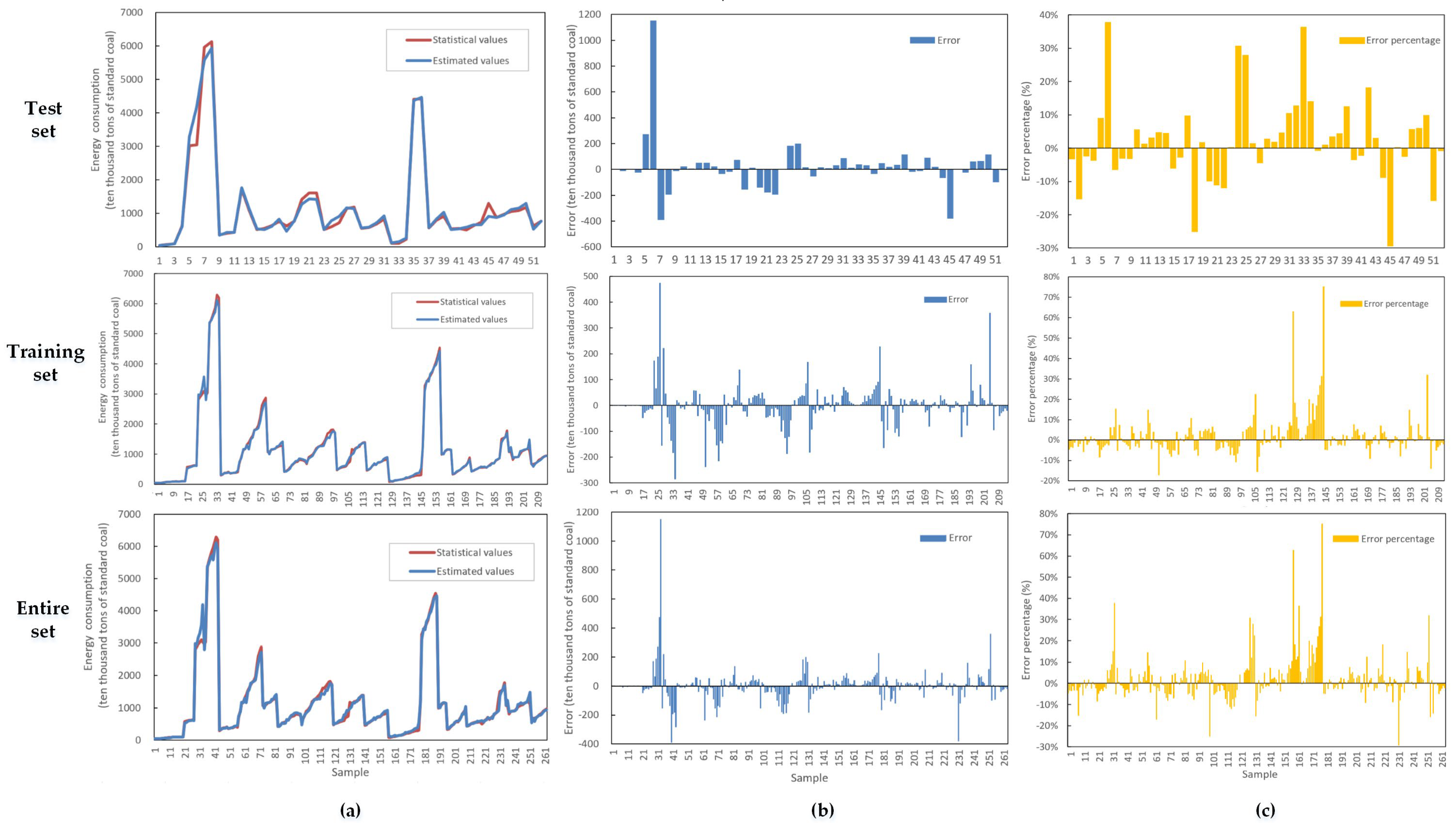
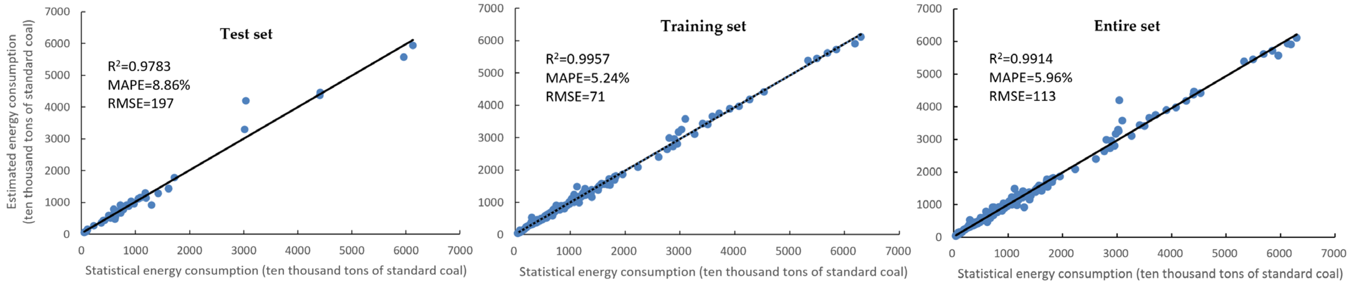
3.1. Results of Model and Accuracy Evaluation

Python 3.9 was used in this study, and the scikit-learn 1.2.0 library was used to train the random forest model and estimate the results. The estimated energy consumption data (unit: ten thousand tons of standard coal) were obtained for each city in Guangdong Province, Hong Kong, and Macao from 2000 to 2020. Figure 5 shows a comparison of the results between the estimated and statistical values of the test set, the training set, and the total set. Figure 5a shows a comparison of the statistical and estimated values for each sample. The difference between the statistical and estimated values is not significant. Figure 5b shows the error values for each sample, while Figure 5c shows the error percentages for each sample, which intuitively demonstrates the individual error situations. The overall distribution of errors appears to be random. In the test set, 27 data points (52%) had error percentages between −5% and 5%, and 37 data points (71%) had error percentages between −10% and 10%. In the training set, 145 data points (69%) had error percentages between −5% and 5%, and 189 data points (90%) had error percentages between −10% and 10%. For the entire set, 172 data points (66%) had error percentages between −5% and 5% and 226 data points (86%) had error percentages between −10% and 10%. It can be observed that the majority of the sampling errors are within 10%, which is the first evidence of a well-estimated result.

Using Equations (1)–(3), R², MAPE, and RMSE were calculated for each dataset. The results are shown in Figure 6. The R² values for the test set, the training set, and the entire set were 0.9783, 0.9957, and 0.9914, respectively. The values were all very close to 1, indicating a well-fitted model. The MAPE values for the test set, the training set, and the entire set were 8.86%, 5.24%, and 5.96%, respectively (all below 10%). According to the evaluation criteria established by C.D. Lewis, these results suggest a high model accuracy, which further confirms the effectiveness of the model.

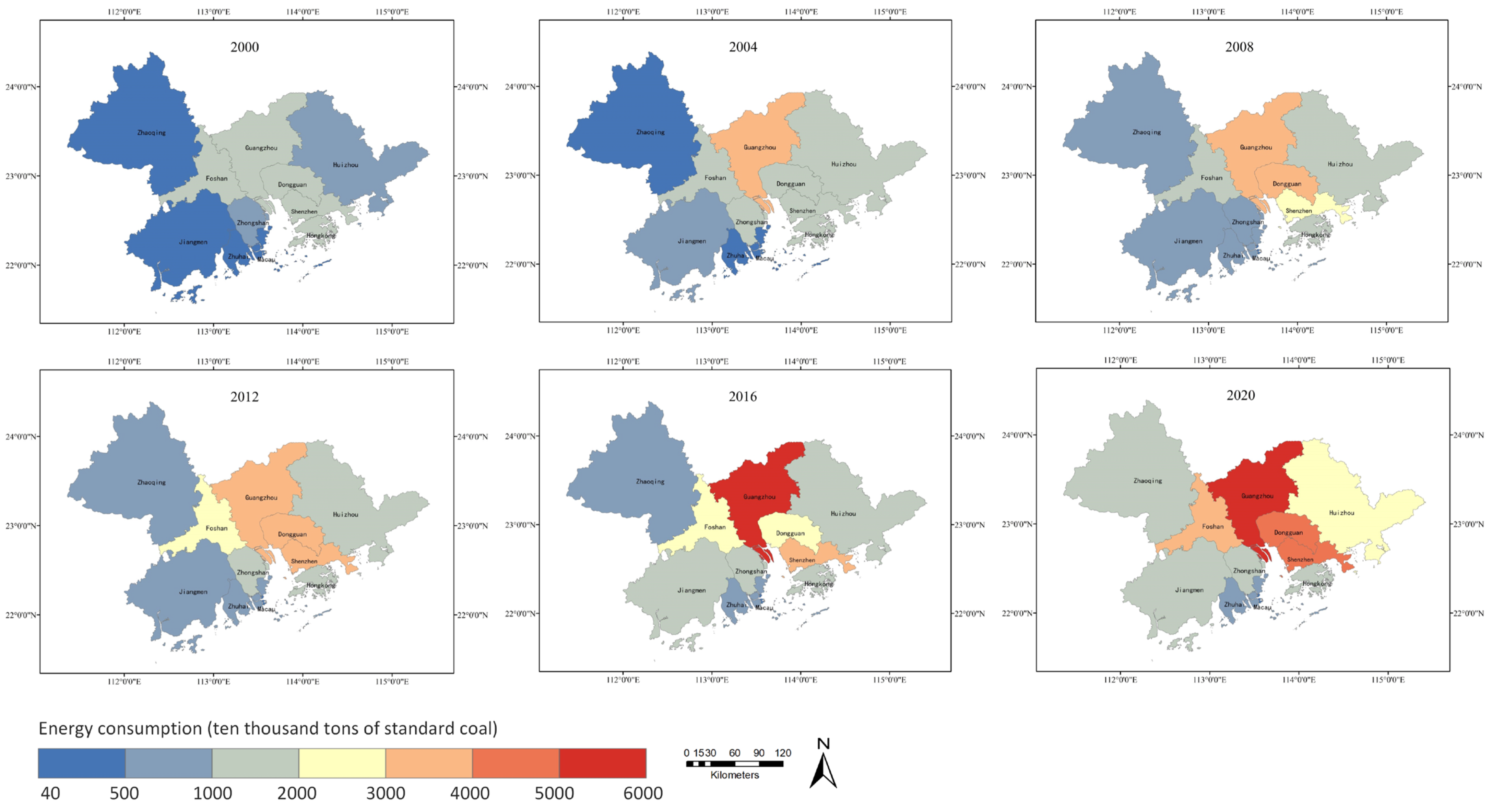
3.2. Spatiotemporal Dynamics of Energy Consumption at the City Scale

The total energy consumption in the Guangdong–Hong Kong–Macao Greater Bay Area increased from 87.94 million tons of standard coal in 2000 to 268.50 million tons in 2020, with a growth rate of about 205%. The growth rate exhibited a trend of a significant increase, followed by a decrease and then another increase. In terms of regions, Guangzhou, Shenzhen, Dongguan, and Huizhou accounted for 72% of the total increase, with Guangzhou making the largest contribution of 24.97% (Figure 7). Using administrative data to spatialize the estimated city-level energy consumption, a map of city-level energy consumption in the Greater Bay Area from 2000 to 2020 was created (Figure 8). It illustrates the growth trend in energy consumption for each city in the 21 years. Guangzhou consistently had the highest energy consumption in the Greater Bay Area, and Shenzhen experienced rapid development. Guangzhou’s surrounding cities also showed high growth in energy consumption, indicating a significant spillover effect from Guangzhou. Looking at the average annual energy consumption (Figure 9a), there are significant differences among cities in the Greater Bay Area, with Guangzhou being 55 times higher than Macao and 7 times higher than Zhuhai. This difference is likely due to differences in the economic and population size of each city. The average annual growth rate of energy consumption (Figure 9b) was over 3% in all cities except Hong Kong. A comparison of the average annual energy consumption and growth rate shows some spatial–temporal characteristics: Guangzhou, Shenzhen, and Dongguan belong to the high consumption and high growth region, Zhuhai and Zhaoqing belong to the low consumption and high growth region, and Foshan belongs to the high consumption and low growth region, while the patterns in other areas are less clear.

3.3. Spatiotemporal Dynamics of Energy Consumption at the Grid Scale

The final random forest model provided importance indices for each feature, with nighttime light density data being 0.16, population density data being 0.41, and urban impervious surface data being 0.43. Equations (4)–(6) were used to calculate the energy consumption values for the 500 × 500 m grid in the Guangdong–Hong Kong–Macao Greater Bay Area for the years 2000 to 2020. Figure 10 shows the distribution of energy consumption in the 500 × 500 m grid in the Greater Bay Area from 2000 to 2020. Compared with the city-level energy consumption map, the grid-level energy consumption map more clearly shows the differences and variations in energy consumption within cities, providing more comprehensive information for the study of energy consumption in urban clusters. The high energy consumption areas are mainly concentrated in the urban areas of Guangzhou, Shenzhen, Hong Kong, and Dongguan and gradually spread out from the central urban areas.

Using the natural breakpoint method, which can maximize the differences between classes with no effect of human factors [45,46], the average energy consumption of the grid in the Greater Bay Area was divided into five levels (Figure 11a), namely, low energy consumption areas, relatively low energy consumption areas, medium energy consumption areas, relatively high energy consumption areas, and high energy consumption areas. The average annual growth rate of energy consumption in the Greater Bay Area grid was divided into four levels (Figure 11b), namely, a no significant growth area, a low growth area, a moderate growth area, and a high growth area. It can be observed that there is a certain negative correlation between energy consumption and energy growth at the grid level, indicating that high energy consumption areas tend to have lower growth rates.

The statistical proportions of energy consumption (Figure 12a) and energy consumption growth (Figure 12b) are shown. The majority of the Greater Bay Area is classified as low energy consumption and relatively low energy consumption areas, with 77.37% and 12.27% of the total area, respectively. Energy consumption is highly concentrated, with approximately 90% of the energy consumption concentrated in 22% of the area (Figure 12a), especially in the relatively high energy consumption and high energy consumption areas, which together account for 3.31% of the total area but account for 32.47% of the energy consumption. The majority of the Greater Bay Area is classified as non-significant growth areas and low growth areas, which account for 83.38% of the total land area and contribute to 90.26% of energy consumption (Figure 12b).

The area proportions of energy consumption levels in each city within the Guangdong–Hong Kong–Macao Greater Bay Area are summarized (Figure 13a), along with the area proportions of energy consumption growth levels in these cities (Figure 13b). The high energy consumption areas are concentrated in Guangzhou, Shenzhen, and Hong Kong, while the low energy consumption areas are concentrated in Zhaoqing, Huizhou, and Jiangmen. The high energy consumption growth areas are concentrated in Guangzhou, Shenzhen, Dongguan, Zhuhai, and Huizhou, while the low energy consumption growth areas are concentrated in Zhaoqing, Huizhou, and Jiangmen. Observing the internal changes within the cities reveals significant variations in energy consumption levels. Shenzhen, for example, has a relatively even distribution across consumption levels, with high energy consumption areas accounting for only a small proportion (3.59%), while the remaining high energy consumption areas account for between 22% and 27%. In contrast, Zhaoqing has a more clustered distribution, with approximately 97% of the area classified as a low energy consumption area. To a certain extent, this reflects the balance of development within cities. However, fine-grained energy consumption data are required to analyze intra-city differences, which emphasizes the importance of compiling energy consumption data with high spatial resolution.

4. Discussion

Nighttime light data are often used to estimate energy consumption data, but previous studies have shown an excessive reliance on nighttime light data, namely, the sole use of nighttime light data to establish energy consumption models. For example, Xiao et al. constructed a spatiotemporal geographically weighted regression model of nighttime light DN values with per capita energy consumption and energy consumption per unit area. Based on this model, they estimated the energy consumption of different provinces in China [19]. Yue et al. used nighttime light data to construct two different models to estimate energy consumption including a quadratic polynomial model and a panel data model. They evaluated the estimation results of the two models based on prefecture-level statistical data. In terms of the accuracy of the results, the panel data model outperformed the quadratic polynomial model [47]. Chen et al. made some improvements by incorporating dummy variables for identity and year as input parameters in addition to the nighttime light data. They used the PSO-BP neural network algorithm to build a provincial-level energy consumption relationship model [48]. In these studies, it was unanimously pointed out in the discussion section that the use of nighttime lighting data as the sole indicator for the estimation models is limited as it may lead to the underestimation of energy consumption data. It was suggested that other indicators such as the level of economic development, population size, and land area should be included in the models. In this study, factors such as nighttime light, population data, and impervious urban surfaces that can influence energy consumption were taken into account. Compared with single-index evaluations, this approach can reflect the actual data situation more comprehensively.

To further validate the accuracy of the model in this study, a comparative analysis was conducted between the estimated total energy consumption of each city in Guangdong Province and the statistical data on energy consumption in Guangdong Province (from the Guangdong Statistical Yearbook). Figure 14 illustrates the results of the comparison. The goodness of fit (R²) between the statistical energy consumption value and the estimated energy consumption value in Guangdong Province is 0.9082, with a mean absolute percentage error (MAPE) of 11.08% (Figure 14a), which further confirms the reliability of our estimates based on the random forest model. The percentage error between the statistical energy consumption value and the estimated energy consumption value in Guangdong Province shows a decreasing trend over time (Figure 14b), which fluctuates in waves. The earlier the time, the larger the percentage error, which is to some extent related to the sample size. A smaller sample size is associated with earlier time points, indicating the importance of sample size in model construction.

In previous simulations of energy consumption, the linear analysis method was mainly used to investigate the relationship between nighttime light data and energy consumption. For example, Yue et al. established a quadratic polynomial model and a panel data model between nighttime light data and energy consumption [47]. Their results showed that the panel data model performed better with a specific R² value of 0.734 and a MAPE of 10.71% for the panel data model compared with an R² of 0.7046 and a MAPE of 18.49% for the quadratic polynomial model. In comparison, the results of the random forest model in our study achieved an R² of 0.9783 and a MAPE of 8.86%. It is evident that the nonlinear model in our study performs better after the effects of nighttime light data, population grid data, and urban impervious surface data are taken into account.

The evaluation of accuracy shows that the constructed random forest model is suitable for predicting energy consumption. However, this study also has certain limitations. First, the estimated results in this study refer to the total energy consumption and not to the energy structure. Different types of energy consumption have different impacts on the atmospheric environment. For example, the combustion of traditional fossil fuels such as coal and oil releases significant amounts of carbon dioxide, sulfur dioxide, particulate matter, and nitrogen oxides, while new and renewable energies do not cause air pollution. Therefore, collecting consumption data for different energy structures can more accurately assess the relationship between energy consumption and air pollution. Secondly, a large amount of training data is required to build the model. However, since there are no statistical data on energy consumption at the city level for the Guangdong–Hong Kong–Macao metropolitan area, the training data in this study are insufficient. Although this study provides good accuracy results at the provincial and city levels, it is difficult to evaluate the model results at the county level because there are no energy consumption data at this level.

5. Conclusions

(1)

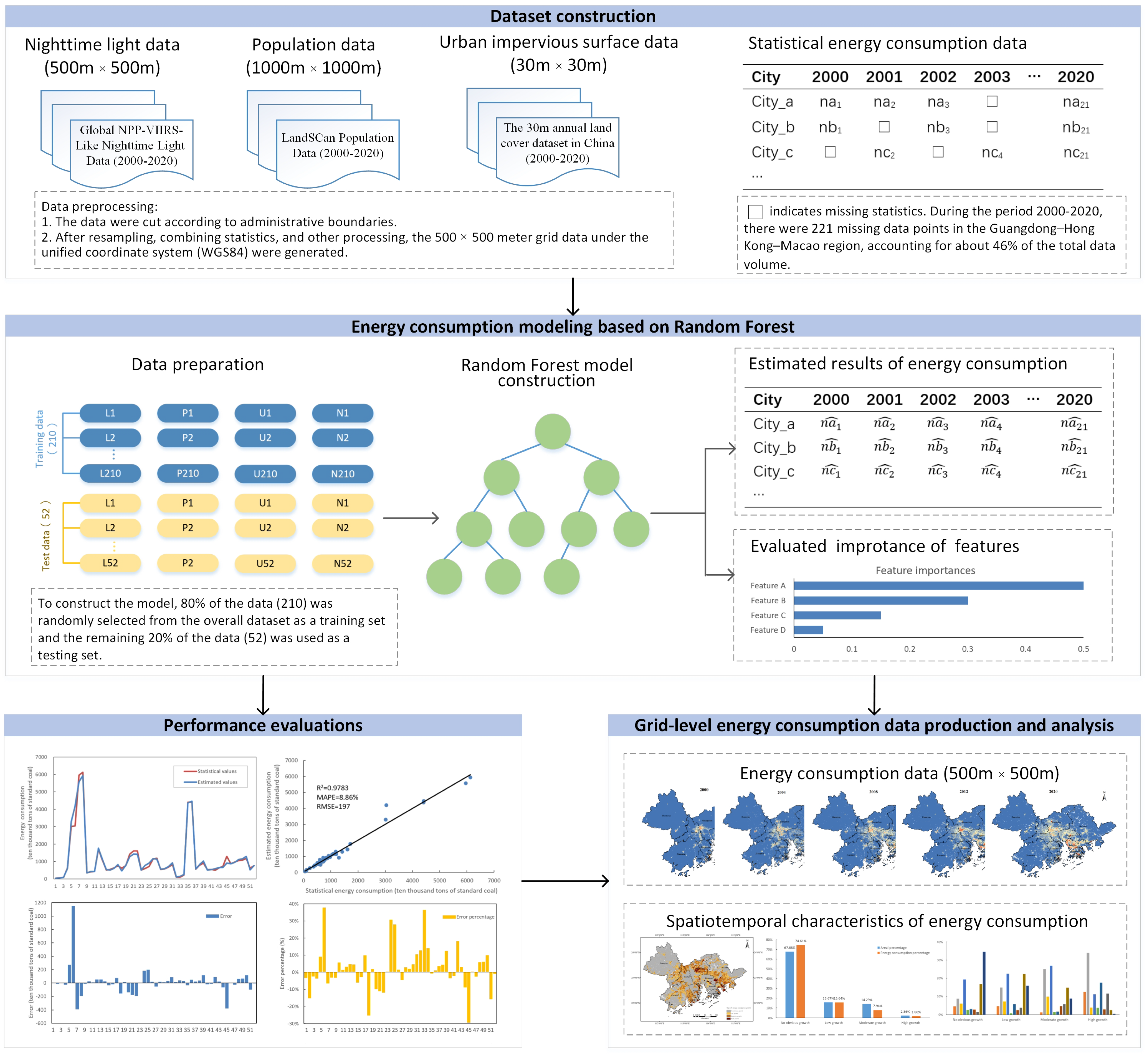
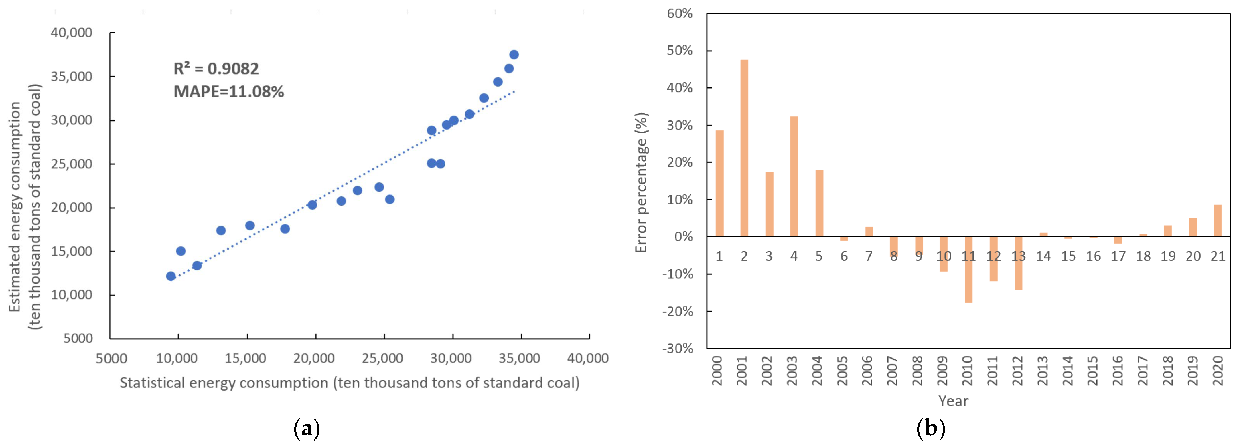
The grid random forest model for estimating metropolitan-level energy consumption shows high accuracy after integrating nighttime light data, population data, and urban impervious surface data in the Guangdong–Hong Kong–Macao Greater Bay Area, with an R² of more than 0.9783 and a MAPE of less than 9%.

(2)

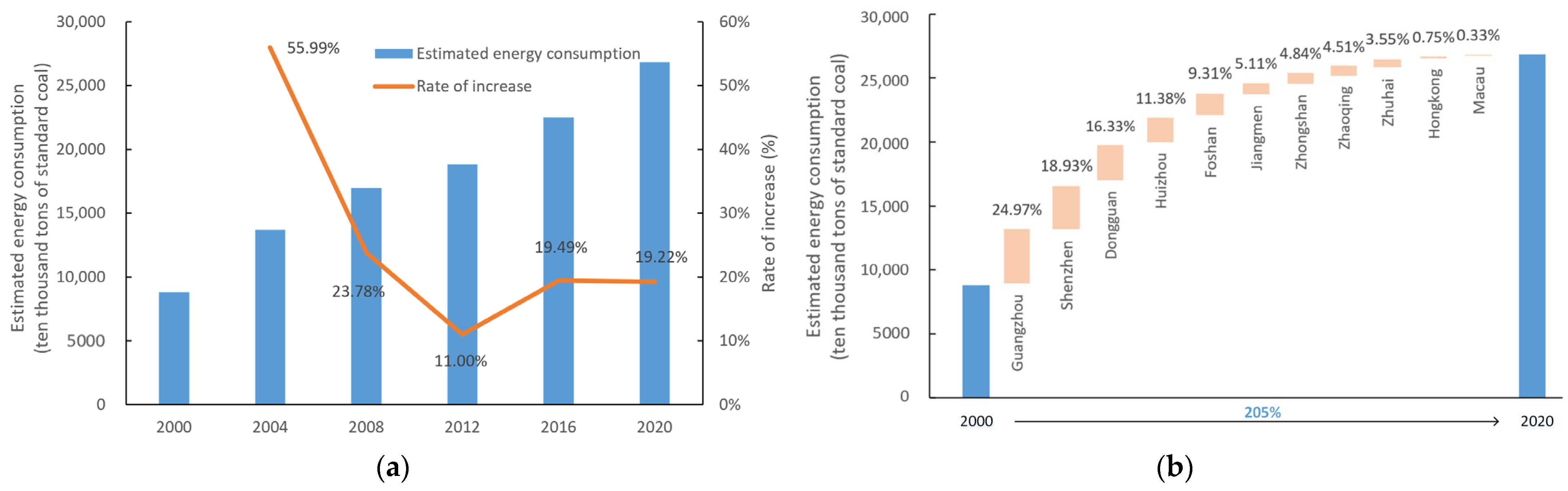
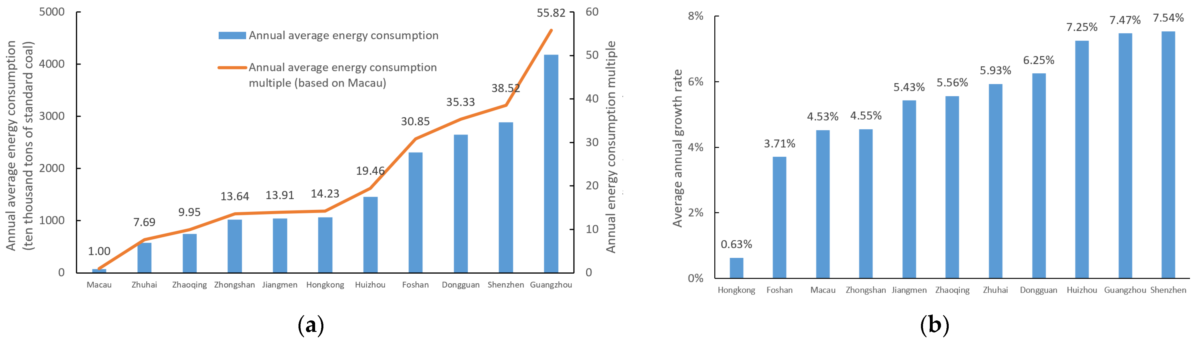
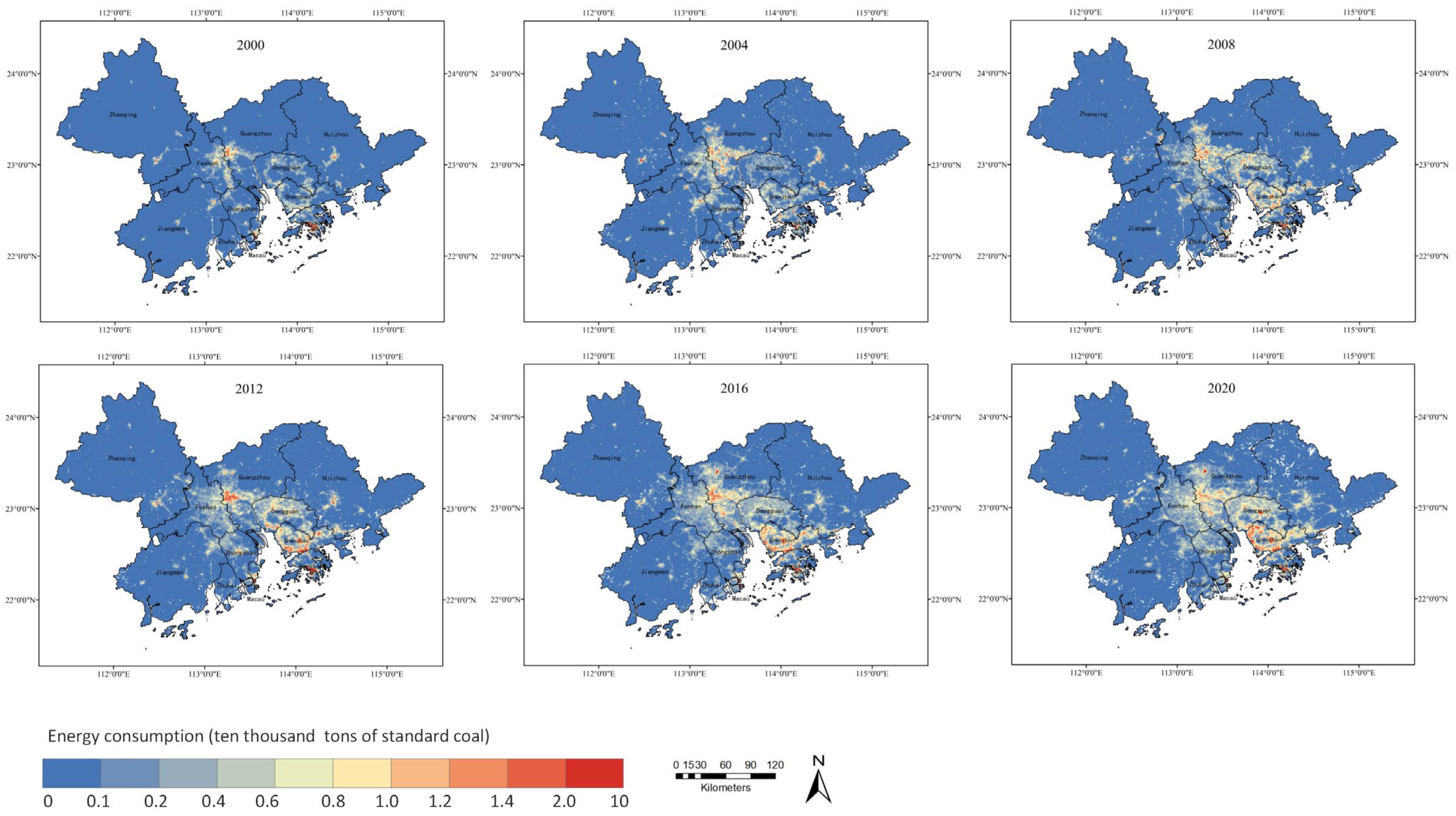
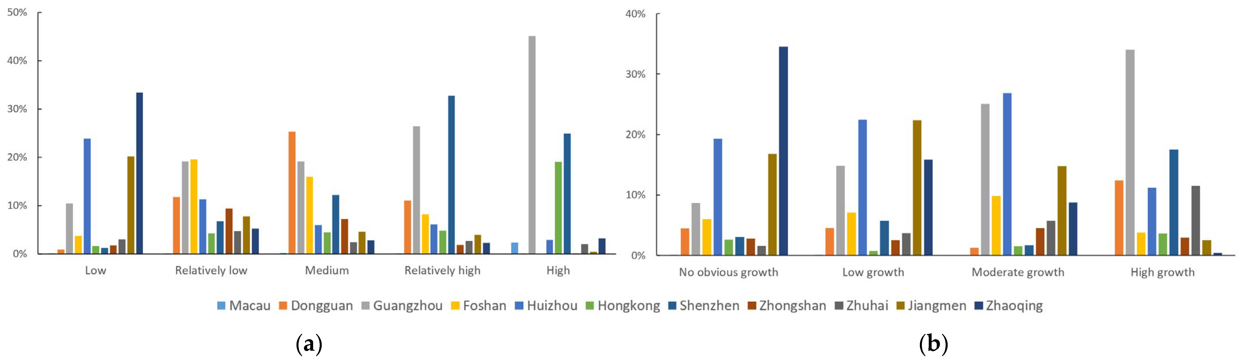
Energy consumption in the study area increased significantly from 2000 to 2020 with a growth rate of about 205%. Guangzhou, Shenzhen, Dongguan, and Huizhou accounted for 72% of the total increase, indicating that these areas had rapid development and high energy consumption.

(3)

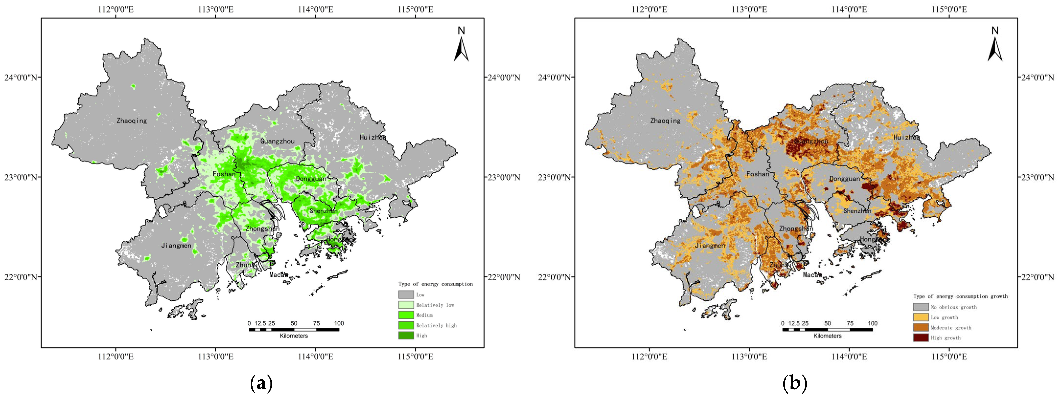
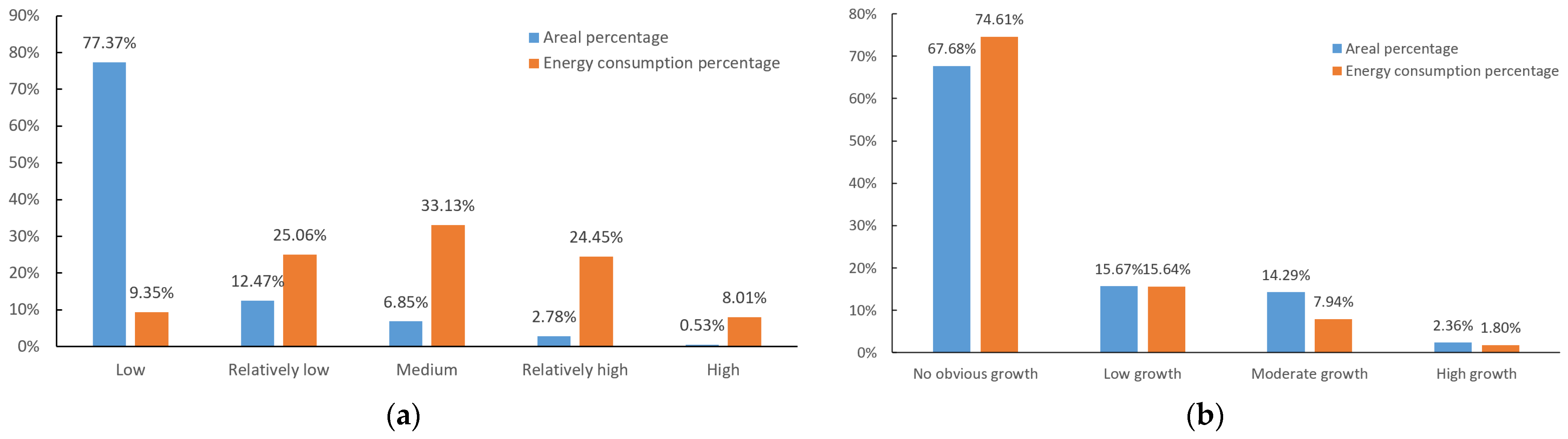
About 90% of the region’s energy consumption was concentrated in only 22% of the area, indicating a pronounced concentration of energy consumption within the Greater Bay Area. This shows that the urban core areas are the main drivers of energy demand and consumption.

(4)

Urban impervious surface data were found to be the most critical factor in predicting energy use (with an importance index of 0.43), indicating the significant impact of urbanization factors, including building density and transportation network completeness, on energy use patterns. This was closely followed by population density data (with an importance index of 0.41), highlighting the role of population distribution in influencing energy demand and consumption. This study shows that areas with a higher population density tend to have higher energy consumption. The importance index of the data on light density was 0.16, which is relatively low. However, there was still a positive correlation between nighttime light brightness and energy consumption.

(5)

The method not only provides a robust framework for estimating energy consumption at the city and grid levels with high spatial resolution but also for monitoring the spatiotemporal evolution of energy consumption. This study could serve as a valuable reference for urban planning and energy policy formulation for sustainable development in regions where detailed energy consumption data are not available.

References

- Banday, U.J.; Aneja, R. Renewable and non-renewable energy consumption, economic growth and carbon emission in BRICS. Int. J. Energy Sect. Manag. 2020, 14, 248–260. [Google Scholar] [CrossRef]
- Bhuiyan, M.A.; Zhang, Q.; Khare, V.; Mikhaylov, A.; Pinter, G.; Huang, X. Renewable energy consumption and economic growth nexus—A systematic literature review. Front. Environ. Sci. 2022, 10, 878394. [Google Scholar] [CrossRef]
- Sahlian, D.N.; Popa, A.F.; Creţu, R.F. Does the Increase in Renewable Energy Influence GDP Growth? An EU-28 Analysis. Energies 2021, 14, 4762. [Google Scholar] [CrossRef]
- Magazzino, C.; Mele, M.; Schneider, N. A machine learning approach on the relationship among solar and wind energy production, coal consumption, GDP, and CO2 emissions. Renew. Energy 2021, 167, 99–115. [Google Scholar] [CrossRef]
- Zhao, J.C.; Liu, Q.Q. Examining the driving factors of urban residential carbon intensity using the LMDI method: Evidence from China’s county-level cities. Int. J. Environ. Res. Public Health 2021, 18, 3929. [Google Scholar] [CrossRef] [PubMed]
- Wang, S.; Li, C.; Zhou, H. Impact of China’s economic growth and energy consumption structure on atmospheric pollutants: Based on a panel threshold model. J. Clean. Prod. 2019, 236, 117694. [Google Scholar] [CrossRef]
- Zheng, W.; Walsh, P.P. Economic growth, urbanization and energy consumption: A provincial level analysis of China. Energy Econ. 2019, 80, 153–162. [Google Scholar] [CrossRef]
- Guo, R.; Yuan, Y. Different types of environmental regulations and heterogeneous influence on energy efficiency in the industrial sector: Evidence from Chinese provincial data. Energy Policy 2020, 145, 111747. [Google Scholar] [CrossRef]
- Li, Y.; Chiu, Y.H.; Lu, L.C.; Chiu, C.R. Evaluation of energy efficiency and air pollutant emissions in Chinese provinces. Energy Effic. 2018, 12, 963–977. [Google Scholar] [CrossRef]
- Bennett, M.M.; Smith, L.C. Advances in using multitemporal nighttime lights satellite imagery to detect, estimate, and monitor socioeconomic dynamics. Remote Sens. Environ. 2017, 192, 176–197. [Google Scholar] [CrossRef]
- McCord, G.C.; Rodriguez-Heredia, M. Nightlights and Subnational Economic Activity: Estimating Departmental GDP in Paraguay. Remote Sens. 2022, 14, 1150. [Google Scholar] [CrossRef]
- Yang, C.; Yu, B.; Chen, Z.; Song, W.; Zhou, Y.; Li, X.; Wu, J. A Spatial-Socioeconomic Urban Development Status Curve from NPP-VIIRS Nighttime Light Data. Remote Sens. 2019, 11, 2398. [Google Scholar] [CrossRef]
- Xie, Y.; Weng, Q. World energy consumption pattern as revealed by DMSP-OLS nighttime light imagery. Mapp. Sci. Remote Sens. 2016, 53, 265–282. [Google Scholar] [CrossRef]
- Welch, R. Monitoring urban population and energy utilization patterns from satellite data. Remote Sens. Environ. 1980, 9, 1–9. [Google Scholar] [CrossRef]
- Amaral, S.; Cmara, G.; Monteiro, A.M.V.; Quintanilha, J.A.; Elvidge, C.D. Estimating population and energy consumption in Brazilian Amazonia using DMSP night–time satellite data. Comput. Environ. Urban Syst. 2005, 29, 179–195. [Google Scholar] [CrossRef]
- Letu, H.; Hara, M.; Yagi, H.; Tana, G.; Nishio, F. Estimating the energy consumption with nighttime city light from the DMSP/OLS imagery. In Proceedings of the 2009 Joint Urban Remote Sensing Event, Shanghai, China, 20–22 May 2009; pp. 1364–1370. [Google Scholar]
- Wu, J.S.; Niu, Y.; Peng, J.; Wang, Z.; Huang, X. Dynamics of Energy Consumption in China’s Prefecture-Level Cities from 1995 to 2009 Based on DMSP/OLS Nighttime Light Data. Geogr. Res. 2014, 33, 625–634. [Google Scholar]
- Bai, C.C. Study on Spatial and Temporal Dynamic Evolution of Energy Consumption in Prefecture-Level City of China Based on Multi-Source Remote Sensing Data. Master’s Thesis, Nanchang University, Nanchang, China, 2016. [Google Scholar]
- Xiao, H.W.; Ma, Z.Y.; Mi, Z.; Kelsey, J.; Zheng, J.; Yin, W.; Yan, M. Spatio–temporal simulation of energy consumption in China’s provinces based on satellite night–time light data. Appl. Energy 2018, 231, 1070–1078. [Google Scholar] [CrossRef]
- Tian, L. Study on Spatio-Temporal Dynamic and Driving Forces of Energy Consumption in China Based on Nighttime Light Data. Master’s Thesis, East China Normal University, Shanghai, China, 2019. [Google Scholar]
- Ou, J.; Liu, X.; Li, X.; Shi, X. Mapping Global Fossil Fuel Combustion CO2 Emissions at High Resolution by Integrating Nightlight, Population Density, and Traffic Network Data. IEEE J. Sel. Top. Appl. Earth Obs. Remote Sens. 2016, 9, 1674–1684. [Google Scholar] [CrossRef]
- Zhao, N.; Liu, Y.; Cao, G.; Samson, E.L.; Zhang, J. Forecasting China’s GDP at the pixel level using nighttime lights time series and population images. GISci. Remote Sens. 2017, 54, 407–425. [Google Scholar] [CrossRef]
- Sun, J.; Di, L.P.; Sun, Z.; Wang, J.; Wu, Y. Estimation of GDP using deep learning with NPP-VIIRS imagery and land cover data at the county level in CONUS. IEEE J. Sel. Top. Appl. Earth Obs. Remote Sens. 2020, 13, 1400–1415. [Google Scholar] [CrossRef]
- Keola, S.; Andersson, M.; Hall, O. Monitoring economic development from space: Using nighttime light and land cover data to measure economic growth. World Dev. 2015, 66, 322–334. [Google Scholar] [CrossRef]
- Chen, Q.; Ye, T.T.; Zhao, N.; Ding, M.; Ouyang, Z.; Jia, P.; Yue, W.; Yang, X. Mapping China’s regional economic activity by integrating points-of-interest and remote sensing data with random forest. Urban Anal. City Sci. 2020, 48, 1–19. [Google Scholar] [CrossRef]
- The State Council of China. Outline Development Plan for the Guangdong-Hong Kong-Macao Greater Bay Area; The State Council of China: Beijing, China, 2019. [Google Scholar]
- Chen, Z.; Yu, B.; Yang, C.; Zhou, Y.; Yao, S.; Qian, X.; Wang, C.; Wu, B.; Wu, J. An Extended Time Series (2000–2018) of Global NPP-VIIRS-Like Nighttime Light Data from a Cross-Sensor Calibration. Earth Syst. Sci. Data 2021, 13, 889–906. [Google Scholar] [CrossRef]
- Bai, Z.Q.; Wang, J.L.; Yang, F. Research progress in spatialization of population data. Prog. Geogr. 2013, 32, 1692–1702. [Google Scholar]
- Bright, E.; Coleman, P.; Dobson, J.E. LandScan: A global population database for estimating populations at risk. Photogramm. Eng. Remote Sens. 2000, 66, 849–858. [Google Scholar]
- Yang, J.; Huang, X. The 30 m annual land cover dataset and its dynamics in China from 1990 to 2019. Earth Syst. Sci. Data 2021, 13, 3907–3925. [Google Scholar] [CrossRef]
- Breiman, L. Random forests. Mach. Learn. 2001, 45, 5–32. [Google Scholar] [CrossRef]
- Moon, J.; Kim, Y.; Son, M.; Hwang, E. Hybrid short-term load forecasting scheme using random forest and multilayer perceptron. Energies 2018, 11, 3283. [Google Scholar] [CrossRef]
- Sun, Z.; Zhao, Y.; Dong, Y.; Cao, X.; Sun, H. Hybrid model with secondary decomposition, random forest algorithm, clustering analysis and long short memory network principal computing for short-term wind power forecasting on multiple scales. Energy 2021, 221, 119848. [Google Scholar] [CrossRef]
- Ye, T.; Zhao, N.; Yang, X.; Ouyang, Z.; Liu, X.; Chen, Q.; Hu, K.; Yue, W.; Qi, J.; Li, Z.; et al. Improved population mapping for China using remotely sensed and points-of-interest data within a random forests model. Sci. Total Environ. 2019, 658, 936–946. [Google Scholar] [CrossRef] [PubMed]
- Iannace, G.; Ciaburro, G.; Trematerra, A. A wind turbine noise prediction using random forest regression. Machines 2019, 7, 69. [Google Scholar] [CrossRef]
- Li, Z.N.; Ye, A.Z. Advanced Econometrics, 1st ed.; Tsinghua University Press: Beijing, China, 2000. [Google Scholar]
- Lewis, C.D. Industrial and Business Forecasting Method, 1st ed.; Butter-Worth Heinemann Press: London, UK, 1982. [Google Scholar]
- Jia, J.P. Fundamentals of Statistics, 1st ed.; Renmin University of China Press: Beijing, China, 2004. [Google Scholar]
- Xiong, P.P.; Dang, Y.G.; Yao, T.X.; Wang, Z.X. Optimal modeling and forecasting of the energy consumption and production in China. Energy 2014, 77, 623–634. [Google Scholar] [CrossRef]
- Gokhan, A. Modeling of energy consumption based on economic and demographic factors The case of Turkey with projections. Renew. Sustain. Energy Rev. 2014, 35, 382–389. [Google Scholar]
- Kummu, M.; Taka, M.; Guillaume, J.H.A. Gridded global datasets for Gross Domestic Product and Human Development Index over 1990–2015. Sci. Data 2018, 5, 180004. [Google Scholar] [CrossRef] [PubMed]
- Balk, D.; Yetman, G. The Global Distribution of Population: Evaluating the Gains in Resolution Refinement; Center for International Earth Science Information Network (CIESIN), Columbia University: New York, NY, USA, 2004. [Google Scholar]
- Balk, D.L.; Deichmann, U.; Yetman, G.; Pozzi, F.; Hay, S.I.; Nelson, A. Determining global population distribution: Methods, applications and data. Adv. Parasitol. 2006, 62, 119–156. [Google Scholar] [PubMed]
- Lei, Y.X. A Study on PM2.5 Prediction Model in Dalian; Dalian Maritime University: Dalian, China, 2021. [Google Scholar]
- Xie, H.L.; He, Y.F.; Zou, J.L.; WU, Q. Spatial–temporal difference analysis of cultivated land use intensity based on emergy in Poyang Lake Eco-economic Zone. J. Geogr. Sci. 2016, 26, 1412–1430. [Google Scholar] [CrossRef]
- Shi, K.; Chen, Y.; Yu, B.; Xu, T.; Chen, Z.; Liu, R.; Li, L.; Wu, J. Modeling spatiotemporal CO2 (carbon dioxide) emission dynamics in China from DMSP-OLS nighttime stable light data using panel data analysis. Appl. Energy 2016, 168, 523–533. [Google Scholar] [CrossRef]
- Yue, Y.; Tian, L.; Yue, Q.; Wang, Z. Spatiotemporal variations in energy consumption and their infuencing factors in China based on the integration of the DMSP-OLS and NPP-VIIRS nighttime light datasets. Remote Sens. 2020, 12, 1151. [Google Scholar] [CrossRef]
- Chen, J.D.; Liu, J.L. City- and county-level spatiotemporal energy consumption and efficiency datasets for China from 1997 to 2017. Sci. Data 2022, 9, 101. [Google Scholar] [CrossRef] [PubMed]