Adaptive Quasi-Super-Twisting Sliding Mode Control for Flexible Multistate Switch

Abstract

The mathematical model of a flexible multistate switch (FMSS) exhibits nonlinear and strong coupling characteristics, whereas traditional power decoupling control makes it difficult to completely decouple the output power. The traditional proportional–integral control parameters are difficult to adjust, and their robustness and dynamic performance are poor, which affects the stability of the voltage of the power distribution network and feeder power. To address these problems, this study first converted the original system into a linear system via coordinate transformation using feedback-accurate linearization to decouple active and reactive currents. Thereafter, a super-twisting sliding mode control (ST-SMC) algorithm was introduced, and an adaptive quasi-super-twisting sliding mode control (AQST-SMC) algorithm comprising the quasi-sliding mode function and adaptive proportional term was proposed. An FMSS double closed-loop controller was designed to achieve improved vibration suppression and convergence speed. A three-port FMSS simulation model was developed using MATLAB/Simulink, and the simulation results show that the proposed control strategy enhances the robustness and dynamic performance of the system.

1. Introduction

With the generalization of distributed energy sources and new types of load access to power systems, traditional distribution networks are experiencing problems such as voltage overruns, bidirectional tidal currents, and feeder power imbalances [1,2,3]. Flexible multistate switches (FMSSs), widely used in medium-voltage distribution grids, can realize continuous and precise power control, improve feeder voltage distribution, and increase the reliability of grid power supply. Furthermore, they can realize a flexible closed-loop operation of the distribution system and increase the ability to consume distributed energy resources [4,5]. Recently, many related studies on FMSSs have been conducted. The proportional–integral (PI) control strategy has been applied [6]; however, this presents challenges, such as difficult parameter adjustment and weak anti-interference ability of multiport FMSSs. In a previous study [7,8], instead of PI control, finite-set model predictive control (MPC) was proposed, which showed excellent dynamic characteristics and anti-interference in a steady state along with a high current response speed. However, such a model presents challenges, such as unstable switching frequency, high control system computation, and model mismatch. Another study [9] proposed an FMSS-based fault detection method for distribution networks under grid-side AC faults, in which the traditional fault management devices were replaced, with the method achieving better dynamic performance during faults. However, the double closed loop still uses PI control, which is parameter-sensitive and insufficiently robust.

FMSSs belong to nonlinear systems exhibiting a strong coupling degree, and it is challenging to design FMSS controllers by applying traditional control theory. When feedback linearization is employed, a nonlinear system can be linearized by selecting an appropriate coordinate mapping method, which can completely decouple the state variables of the system, thus considerably improving the control performance of the system [10]. Sliding mode control (SMC) is a nonlinear control method that requires a model exhibiting high accuracy but considerably short response time and high robustness; it has been widely used in the design of FMSS controllers and observers. In a previous study, second-order SMC was combined with a nonlinear disturbance observer to design a strategy for suppressing direct current (DC)-side voltage fluctuations caused by the voltage imbalance of FMSS ports [11], which resulted in accurate tracking of the reference voltage and current. However, the nonlinear disturbance observer was sensitive to the system model error and parameter perturbation, and exhibited poor robustness. A soft open point (SOP) strategy based on adaptive voltage drop outer-loop control and feedback-linearized sliding mode inner-loop control was proposed to fully harness the regulation capability of the converter in the SOP system to avoid reaching the voltage limit [12]. Furthermore, the strategy was proposed to balance the tidal current in the distribution network. However, the inner loop uses a conventional first-order linear sliding mode, which may not be sufficiently robust to external perturbations and uncertainties, leading to a decline in the control system’s performance. A full-order terminal SMC method was proposed to enhance system immunity to disturbances by establishing a mathematical FMSS model considering parameter uptake [13]. However, the full-order terminal sliding mode response was slower in the initial moments and cases of large nonlinear disturbances. The super-twisting SMC (ST-SMC) algorithm is a second-order sliding mode algorithm. This algorithm only uses information about the system state and its first-order derivatives in designing the system control law, and can be directly used to design controllers and observers for relative-degree-one systems, which makes it widely applicable in second-order sliding mode control [14]. Moreover, it is more accurate and robust than first-order SMC. Furthermore, extensive research has been conducted on the mathematical computation of ST-SMC algorithms. Xu et al. proposed a variable-step closed-loop angle compensation method using the tangent reaching law based on SMC and the convergence law. Results revealed that the algorithm exhibited good dynamic compensation performance and disturbance resistance while maintaining good steady-state compensation accuracy [15]. Maged et al. proposed a new application of ST-SMC based on an artificial hummingbird optimization technique, in order to enhance the transient performance of islanded microgrids [16]. Ghazi et al. proposed an ST algorithm based on the circle search algorithm to improve the efficiency of grid-connected photovoltaic systems; its parameters were optimized in combination with the gray wolf optimizer to improve the robustness of the system, tracking speed, and the optimal convergence to the minimum error value [17].

In recent years, ST-SMC has been widely used in power electronics and power drives; moreover, considerable research has focused on improving the traditional ST-SMC by combining it with other nonlinear control algorithms to optimize the dynamic and steady-state characteristics of the system. Saadaoui et al. proposed an ST-SMC method for ultrafast chargers of pure electric vehicles for grid imbalance conditions, which can always achieve the lowest performance index compared with other nonlinear methods, demonstrating the fast response speed, strong robustness, and low steady-state error of ST-SMC [18]. Celik et al. designed a Kalman filter using an ultra-twisted sliding-mode strategy, which ensures a shallow DC-link voltage ripple and achieves a fast dynamic response for a battery electric vehicle charger based on a three-phase two-level rectifier and a conventional DC/DC buck-boost converter [19]. Tiwary et al. designed an ST-SMC controller based on an isolated DC–DC bidirectional dual active bridge (DAB) power converter, in order to achieve DC bus voltage stability and high robustness for accurate reference voltage tracking [20].

To enhance the performance of the control system in complex environments, some improved ST-SMCs have been created. Wang et al. proposed a model-free predictive current control strategy based on an adaptive super-twisting sliding-mode observer, in order to design an adaptive gain matrix and dynamically adjust the observer parameters to suppress the effect of boundary uncertainty in the dynamic part of the rectifier system, and to ensure the accuracy of the prediction model [21]. Pati et al. proposed adaptive ST-SMC and dual-loop control for a three-phase differential boost inverter in a grid-connected photovoltaic system to regulate voltage across a DC bus capacitor, and to compensate for harmonics under nonlinear loads [22]. However, for FMSS systems, ST-SMC exhibiting improved efficiency should be developed to withstand various complex operating conditions, and exhibit enhanced dynamic performance in complex environments. Composite second-order SMC was proposed to apply ST-SMC in the outer loop of an FMSS [23]. Nevertheless, the full-order fast terminal SMC used in the inner loop requires high model accuracy, is sensitive to measurement errors, and is prone to cause instability in the controller’s performance. Another paper [24] proposed an ST sliding-mode observer to improve the immunity of an FMSS system, and applied the conventional ST-SMC to design a voltage outer-loop controller to enhance its dynamic performance and robustness. However, the inner loop was poorly controlled using three-vector MPC, which requires high system data accuracy and complex computation.

In this study, a linear radiation model of a three-terminal FMSS was first obtained by applying the exact feedback linearization method, which decouples active and reactive currents. Subsequently, an adaptive QST-SMC (AQST-SMC) algorithm was proposed to design the voltage outer-loop and current inner-loop controllers of the three-terminal FMSS. The algorithm adopted the sigmoid function in the quasi-sliding mode to discretize the switching function and reduce the jitter. An adaptive scaling term was introduced to adjust the response speed of the system, which considerably shortens its response time and enhances immunity to interference. Finally, a three-terminal FMSS simulation model was constructed to verify the effectiveness of the proposed AQST-SMC strategy.

The rest of the paper is organized as follows: Section 2 describes the establishment of an affine nonlinear model of the FMSS system, which provides the basis for the subsequent construction of an AQST-SMC controller. Section 3 explains the construction of the AQST-SMC controller and compares it with conventional control strategies, such as first-order SMC. Section 4 describes the construction of the voltage outer-loop and current inner-loop controllers based on a radiative nonlinear model and mathematical equations of the FMSS system. Section 5 presents the establishment of a simulation of the three-terminal FMSS system, and the verification of its performance under different operating conditions. Section 6 presents the conclusions of this study.

2. FMSS Nonlinear Control Design

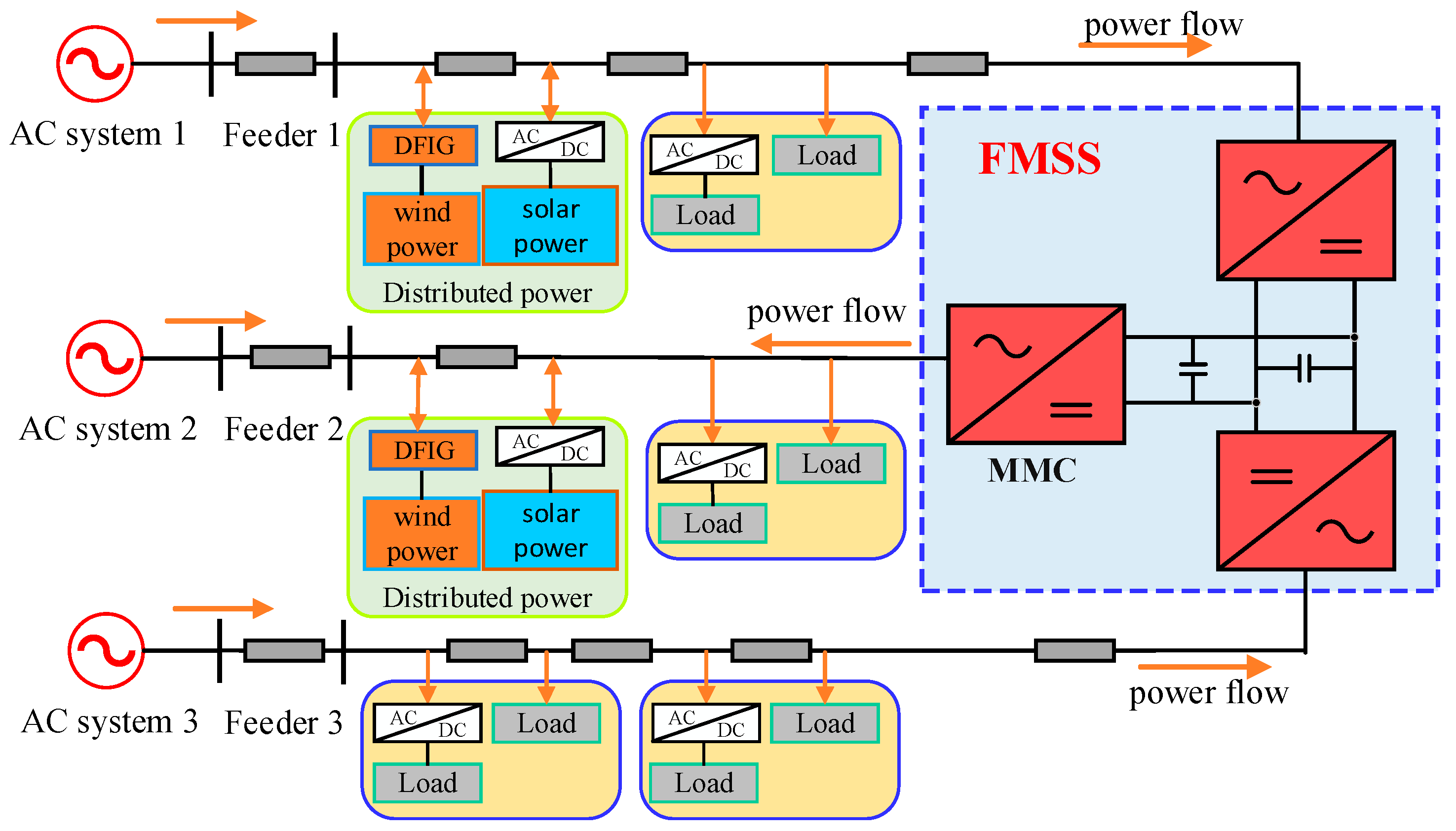
2.1. FMSS System Architecture

In medium-voltage distribution networks, feeders of different voltage levels are connected through an FMSS. However, with the upgrade and transformation of these distribution networks and the rapid development of loads, double-ended flexible switchgear cannot fulfill the requirements of the interconnection of multi-distribution areas in complex environments. In addition, the switchgear cannot regulate the power between the feeders if one of the ports fails. Therefore, it is important to study three-port and multiport FMSSs. A three-port FMSS can connect multiple feeders and reduce the construction cost. In addition, if one end is out of operation owing to failure, the rest of the converter can flexibly switch the working mode to support the normal operation of the power grid, which is more reliable. Figure 1 shows the structure of the three-terminal FMSS system mentioned earlier. For each feeder, the head of the transmission line is typically connected to the substation. Thus, the AC system connected to the FMSS can be equated to a Davignon equivalent circuit comprising a fixed alternating current (AC) voltage source and a series impedance at the point of common coupling.

Modular multilevel converters (MMCs) are widely used in power electronics, owing to their small loss and good quality of voltage and current waveforms generated by power conversion in the working state [25]. Thus, this study used MMCs as the main circuit topology.

2.2. FMSS Radiation Modeling

Assuming the AC system is balanced in three phases, the MMC equation of state was obtained from the circuit law as follows:

$$L\frac{d}{dt}\left[\begin{array}{l}{i}_{sd}\\ i_{sq}\end{array}\right]=\left[\begin{array}{cc}-R& \omega L\\ -\omega L& -R\end{array}\right]\left[\begin{array}{l}{i}_{sd}\\ i_{sq}\end{array}\right]+\left[\begin{array}{cc}{u}_{sd}& -m_d{U}_{\mathrm{dc}}\\ u_{sq}& -m_q{U}_{\mathrm{dc}}\end{array}\right],$$

(1)

where ω represents the AC voltage angular frequency. In the rotating coordinate system, i_sd i_sq and u_sd u_sq represent the output current and voltage of any phase of the port, respectively. Moreover, m_d m_q represents the modulation switching function components of any phase of the port.

The transformation of (1) yielded the following nonlinear radiation model of the FMSS system:

$$\left\{\begin{array}{l}\dot{\mathit{x}}=\mathit{f}(\mathit{x})+\mathit{g}(\mathit{x})\mathit{u}\\ \mathit{y}=\mathit{h}(\mathit{x})\end{array}\right.,$$

(2)

$$\mathit{f}\left(\mathit{x}\right)=\left[\begin{array}{l}{\mathit{f}}_1\left(\mathit{x}\right)\\ {\mathit{f}}_2\left(\mathit{x}\right)\end{array}\right]=\left[\begin{array}{l}-\frac{R}{L}{x}_1+\omega x_2+\frac{u_{sd}}{L}\\ -\frac{R}{L}{x}_2-\omega x_1+\frac{u_{sq}}{L}\end{array}\right],$$

(3)

$$\mathit{g}\left(\mathit{x}\right)={\left[\begin{array}{l}{\mathit{g}}_1\left(\mathit{x}\right)\\ {\mathit{g}}_2\left(\mathit{x}\right)\end{array}\right]}^{\mathrm{T}}=\left[\begin{array}{cc}-\frac{U_{\mathrm{dc}}}{L}& 0\\ 0& -\frac{U_{\mathrm{dc}}}{L}\end{array}\right],$$

(4)

where x = [x₁, x₂]^T = [i_sd, i_sq]^T, u = [u₁, u₂]^T = [m_d, m_q]^T, and y = [y₁, y₂]^T. h(x) satisfies h(x) = [h₁(x), h₂(x)]^T = [i_sdref−x₁, i_sqref−x₂]^T, and i_sdref, i_sqref denotes the inner-loop current reference.

The Lie derivative of function h(x) along the vector field f(x) is defined as follows:

$$L_{f(x)}{h}_i(x)=\frac{\partial h_i(x)}{\partial x}\mathit{f}(x).$$

(5)

From (5), we obtain the following:

$$L_{g_i\left(x\right)}{L}_{f(x)}{h}_i(x)=\frac{\partial L_{f(x)}{h}_i(x)}{\partial x}{\mathit{g}}_i\left(x\right).$$

(6)

According to the differential geometry theory, the nonlinear radiation model satisfies the following constraints, and the matrix, B(x), is nonsingular:

$$\left\{\begin{array}{l}{L}_{f\left(x\right)}^k{h}_i\left(x\right)=L_{f\left(x\right)}\left(L_{f\left(x\right)}^{k-1}{h}_i\left(x\right)\right)\\ L_{g_i\left(x\right)}{L}_{f\left(x\right)}^k{h}_j\left(x\right)=0\\ L_{f\left(x\right)}^0{h}_i\left(x\right)=h_i\left(x\right)\\ L_{g_i\left(x\right)}{L}_{f\left(x\right)}^{r_j-1}{h}_j\left(x\right)\ne 0\end{array}\right.k=1,2,\cdots i,j=1,2.$$

(7)

$$\mathit{B}(\mathit{x})=\left[\begin{array}{cc}{L}_{g_1\left(x\right)}{L}_{f\left(x\right)}^{r_1-1}{h}_1\left(x\right)& L_{g_2\left(x\right)}{L}_{f\left(x\right)}^{r_1-1}{h}_1\left(x\right)\\ L_{g_1\left(x\right)}{L}_{f\left(x\right)}^{r_2-1}{h}_2\left(x\right)& L_{g_2\left(x\right)}{L}_{f\left(x\right)}^{r_2-1}{h}_2\left(x\right)\end{array}\right]=\left[\begin{array}{cc}\frac{U_{\mathrm{dc}}}{L}& 0\\ 0& \frac{U_{\mathrm{dc}}}{L}\end{array}\right],$$

(8)

where r = [r₁, r₂] corresponds to the subrelativity of function h(x).

When the FMSS satisfies the normal operation of the aforementioned equation and r₁ + r₂ = 2 is equal to the order of the system, the choice of coordinate transformation can fully linearize the nonlinear model of the FMSS.

2.3. Coordinate Mapping and Control Law Solving

The following coordinate transformation matrix was selected:

$$\mathit{z}=\left[\begin{array}{l}{z}_1\\ z_2\end{array}\right]=\left[\begin{array}{l}{h}_1\left(\mathit{x}\right)\\ h_2\left(\mathit{x}\right)\end{array}\right]=\left[\begin{array}{l}{i}_{sd\mathrm{ref}}-x_1\\ i_{sq\mathrm{ref}}-x_2\end{array}\right].$$

(9)

The control variable after the exact feedback linearization takes the following form:

$$\mathit{\nu }=\mathit{A}\left(\mathit{x}\right)+\mathit{B}\left(\mathit{x}\right)\mathit{u}+\frac{R}{L}\mathit{z}.$$

(10)

$$\mathit{A}\left(\mathit{x}\right)=\left[\begin{array}{l}{L}_{f\left(x\right)}^{r_1-1}{h}_1\left(x\right)\\ L_{f\left(x\right)}^{r_2-1}{h}_2\left(x\right)\end{array}\right]=\left[\begin{array}{l}\frac{R}{L}{x}_1-\omega x_2-\frac{u_{sd}}{L}\\ \frac{R}{L}{x}_2+\omega x_1-\frac{u_{sq}}{L}\end{array}\right].$$

(11)

The reintegrated linear system was as follows:

$$\mathit{u}={\mathit{B}}^{-1}\left(\mathit{x}\right)\left[\mathit{\nu }-\mathit{A}\left(\mathit{x}\right)-\frac{R}{L}\mathit{z}\right].$$

(12)

$$\mathit{u}=\left[\begin{array}{l}{m}_d\\ m_q\end{array}\right]=\left[\begin{array}{l}\frac{L}{U_{\mathrm{dc}}}\left({\nu }_1+\omega x_2+\frac{u_{sd}}{L}\right)-\frac{R}{U_{\mathrm{dc}}}{i}_{sd\mathrm{ref}}\\ \frac{L}{U_{\mathrm{dc}}}\left({\nu }_2-\omega x_1+\frac{u_{sq}}{L}\right)-\frac{R}{U_{\mathrm{dc}}}{i}_{sq\mathrm{ref}}\end{array}\right].$$

(13)

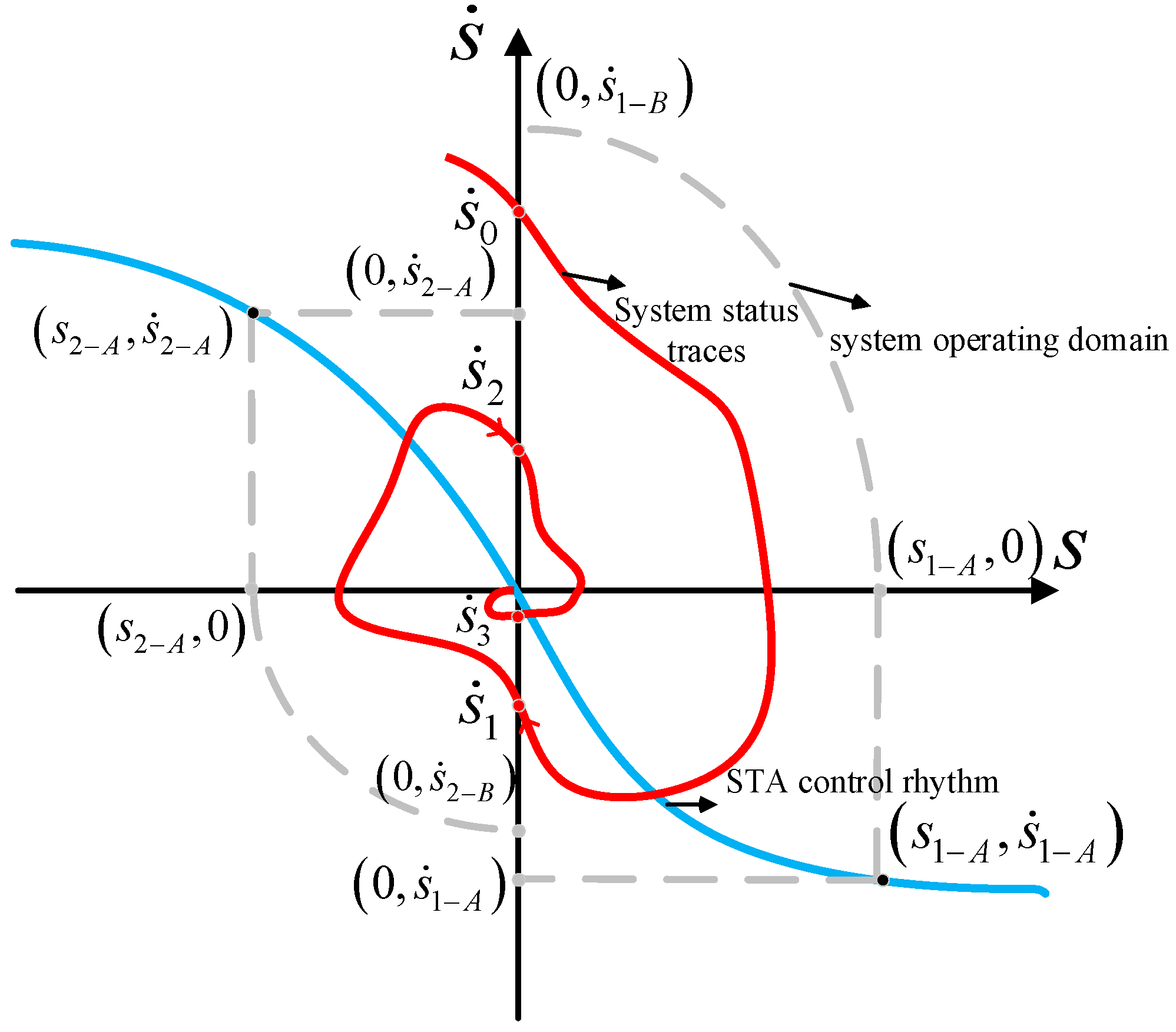
3. Construction of Adaptive Quasi-Super-Twisting Sliding Mode Controller

Second-order SMC uses the differentiation of the control input as a new virtual control quantity, and applies it to the higher-order derivatives of the sliding mode surface to ensure that the sliding variable, s, converges to zero in a restricted time [26]. This weakens the jitter, eliminates relative-order limitations, and improves the accuracy and reliability of the SMC.

The super-twisting algorithm (STA) is a second-order SMC algorithm designed for systems of relative order 1, which ensures that the system reaches the ideal state (s). Its first-order derivative is zero in a finite time. Conversely, conventional first-order SMC can only render the system state (s) zero in a finite time. The general expression of the STA is as follows:

$$\left\{\begin{array}{l}u=-\alpha {\left|s\right|}^{1/2}\mathrm{sign}\left(s\right)+u_1\\ {\dot{u}}_1=-\beta \mathrm{sign}\left(s\right)+\dot{\phi }\end{array}\right.,$$

(14)

where s represents a sliding variable; u₁ represents an auxiliary variable; φ represents a perturbation term; and α and β represent sliding mode gain coefficients.

If (14) satisfies $\left|\dot{\phi }\right|\le \delta$ and $\delta >0$, then α and β simultaneously satisfying the following conditions can cause (14) to converge in a finite time [27].

$$\left\{\begin{array}{l}\alpha >2\\ \beta >\frac{{\alpha }^3+\left(4\alpha -8\right){\delta }^2}{\alpha \left(4\alpha -8\right)}\end{array}\right..$$

(15)

Figure 2 shows the phase plane trajectory of the STA, and point S_1−A is the intersection of the system-state trajectory curve with the axis, $\dot{s}=0$ and $2\left(K_{1-A}^{\prime }\beta -L\right)s_{1-A}={\dot{s}}_0^2$, where $K_{1-A}^{\prime }$ and L are positive constants. The calculation shows that ${\dot{s}}_{1-A}=-\frac{2}{\alpha }\left(\frac{L}{K_{1-A}^{\prime }}+\beta \right)s_{1-A}^{1/2}$, which affords $\left|{\dot{s}}_{1-A}\right|/\left|{\dot{s}}_0\right|<1$. Considering that $\left|{\dot{s}}_1\right|\le \left|{\dot{s}}_{1-A}\right|$, $\left|{\dot{s}}_1\right|/\left|{\dot{s}}_0\right|<1$ holds; repeating the process ensures the inequality $\left|{\dot{s}}_{k+1}/{\dot{s}}_k\right|=\left|{\dot{s}}_{k+1}\right|/\left|{\dot{s}}_k\right|<1$ holds. Similarly, it can be shown that $\left|s_{k+1}/s_k\right|=\left|s_{k+1}\right|/\left|s_k\right|<1$ holds, indicating that the closed-loop system can converge to stability in a finite time [28].

Based on (14), the introduction of the integral term can effectively attenuate the jitter and eliminate the static error of the system. However, there is still a sign function with poor smoothing performance near the sliding mode surface in the control law. This can cause high-frequency jitter with rapid and frequent switching on the sliding mode surface, and reduce the control accuracy of the system. A study [29] added a sinusoidal saturation function, sat (s), in the super-twisting control law to reduce the system jitter. However, the saturation function presents the problem of selecting the appropriate thickness of the boundary layer, which is extremely large to lead to the insufficient control accuracy of the system, and excessively small to cause oscillations. Thus, the following smoother sigmoid function was designed:

$$\mathrm{sd}\left(s\right)=\frac{2}{1+{\mathrm{e}}^{-ns}}-1.$$

(16)

A constant (n > 0) was used to adjust the rate of the curve rise, which determines the function boundary layer thickness. Figure 3 shows that the sign function changes stepwise at t = 0, and that the sigmoid function continuously and smoothly changes with the input. The quasi-smooth mode changes more gradually than the switching function, which can alleviate the shock of the smooth mode switching and reduce the appearance of high-frequency jitter to a certain extent. This can improve the response speed and control accuracy of the FMSS system.

Equation (14) shows that the proportional term, $-\alpha {\left|s\right|}^{1/2}sign(s)$, improves the convergence speed of the algorithm. However, the exponent of the state vector is always 1/2, which prevents the system state from converging to a smaller region. The immunity of the algorithm to interference and the arrival speed are directly affected by its gain. A previous study [18] introduced the proportional term in a traditional STA to improve the convergence trajectory of the system. However, when s < 1, i.e., ks is zero; the proportional term is only left with the original square root term, and the problem of low arrival speed remains. To solve the aforementioned problem, this study introduced an adaptive linear term to realize the adaptive regulation of the convergence speed with the following expression:

$$q\left(s\right)=k{\left|s\right|}^{c\cdot \mathrm{sign}\left(\left|s\right|-1\right)}s,$$

(17)

where k > 0, 0 < c < 1. When the system state tends to the sliding mode surface, i.e., s < 1, the adaptive term becomes $q\left(s\right)=k{\left|s\right|}^{-c}s$, $\alpha {\left|s\right|}^{1/2}\mathrm{sign}\left(s\right)+k{\left|s\right|}^{-c}s\gg \alpha {\left|s\right|}^{1/2}\mathrm{sign}\left(s\right)$, which speeds up the convergence. Furthermore, when the system state tends to the sliding mode surface, i.e., s > 1, the adaptive term becomes $q\left(s\right)=k{\left|s\right|}^{c}s$, $\alpha {\left|s\right|}^{1/2}\mathrm{sign}\left(s\right)+k{\left|s\right|}^{c}s\gg \alpha {\left|s\right|}^{1/2}\mathrm{sign}\left(s\right)$, which speeds up the convergence.

Using the sigmoid function and adaptive scaling term, the AQST-SMC mathematical expression can be written as follows:

$$\left\{\begin{array}{l}u=-\alpha {\left|s\right|}^{1/2}\mathrm{sd}\left(s\right)-q\left(s\right)+\omega \\ \dot{\omega }=-\beta \mathrm{sd}\left(s\right)+\dot{\phi }\\ q\left(s\right)=k{\left|s\right|}^{c\cdot \mathrm{sign}\left(\left|s\right|-1\right)}s\end{array}\right..$$

(18)

If (18) satisfies $2\left|\dot{\phi }\right|\le \delta$ and $\sigma >0$, then α, β, and k simultaneously satisfying condition (19) can cause (18) to converge to the origin in a finite time. The stability of the AQST-SMC algorithm was confirmed, as described in Appendix A. It was discovered that the stability of the system will not be affected by the introduction of the adaptive linear term, q(s), into the super-twisting algorithm, as long as it is guaranteed that k > 0.

$$\left\{\begin{array}{l}\alpha >2\\ \beta >\frac{{\left(\alpha +k{\left|x_1\right|}^{1/2}\right)}^2}{4{\left(\alpha +k{\left|x_1\right|}^{1/2}\right)}^2-8}+\frac{{\delta }^2}{4\alpha }\\ k>0\end{array}\right..$$

(19)

To verify the effectiveness of the proposed AQST-SMC, it was compared with the conventional first-order SMC, conventional STA, and STA without the adaptive acceleration term. Figure 4 and Figure 5 show the comparison results. First-order SMCs can usually reach the sliding mold surface in finite time. Nevertheless, they cannot maintain stability and equilibrium, and most conventional first-order SMCs are less efficient than second-order SMCs in terms of control performance and the tracking error, as shown in Figure 4a,b; the tracking accuracy and convergence speed of conventional first-order SMCs are worse than those of the conventional ST-SMC and the ST-SMC that contains only the sigmoid function. Using the designed adaptive convergence term equation q(s), the AQST-SMC can approach the surface of the sliding mode quickly, and the system’s state variables can converge smoothly. From Figure 5, the introduction of the continuous smooth sigmoid function attenuates the system’s jitter and enhances the system’s perturbation resistance compared to the sign function, confirming the effectiveness of the AQST-SMC.

Owing to the limitation of the stability condition Equation (19), control gain k must be selected within a certain range. When k is excessively small, the adaptive term q(s) tends to zero, thus preventing the achievement of the desired acceleration effect and simultaneously departing from the limitations of the stability condition. This causes the system trajectory to deviate from the sliding mode surface; however, although the convergence speed increases when k becomes larger, it may cause new problems such as considerable overshooting or system oscillations due to the integral term. Therefore, k must be designed in a reasonable range to ensure that the system state variables converge smoothly in a stable range. Figure 4c,d show simulations that were conducted to test the effect of different gain coefficients k on the convergence of the system state to the surface of the sliding mode. When a higher value of k is considered (e.g., k = 200), the convergence is fast; thus, oscillations may occur. Conversely, when a small value of k is considered (e.g., k = 2 or 5), the system state does not reach the surface of the sliding mode completely, but the convergence speed is still faster than that of the conventional ST-SMC. Notably, in Figure 4, the three ST-SMCs use the same gain coefficients. Conversely, traditional first-order SMCs use the integral sliding mode surface and the exponential convergence law. Their gain parameters are selected to ensure that the system reaches the surface of the sliding mode in a finite amount of time and remains stable.

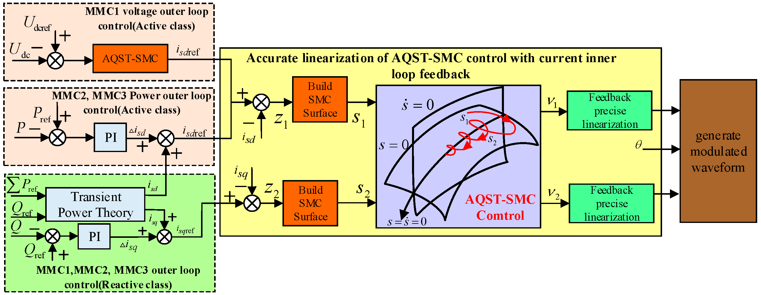
4. FMSS AQST-SMC Controller Design

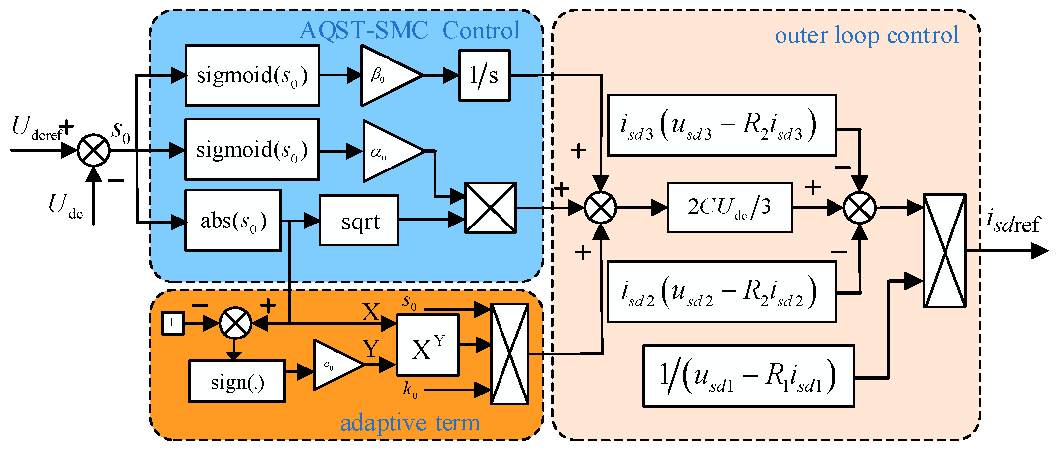
4.1. AQST-SMC Voltage Outer Ring Design

During normal operation, the FMSS needs to operate in the U_dcQ mode at one end to maintain a constant voltage on the DC side. The remaining ports operate in the PQ mode for power exchange. However, in the traditional outer-loop PI controller, when the system parameters are changed, the dynamic performance and response time of the system will increase because of the constant parameters of the PI. In this research, the AQST-SMC was designed to effectively suppress the jitter and speed up the response; it exhibits good dynamic performance and response time. The steady-state inverse model [7] was used to improve the traditional power outer-loop controller, which improves the outer-loop regulation rate and eliminates the static error of the system. For example, this study analyzed MMC1 running in the U_dcQ operation mode, and MMC2 and MMC3 running in the PQ mode.

First, the three-port FMSS DC side satisfied (20), as follows:

$$\left\{\begin{array}{l}C\frac{d{U}_{\mathrm{dc}}}{dt}=i_{\mathrm{dc}1}+i_{\mathrm{dc}2}+i_{\mathrm{dc}3}={\displaystyle \sum _{k=1}^3{i}_{\mathrm{dc}k}}\\ i_{\mathrm{dc}k}=m_{ak}{i}_{ak}+m_{bk}{i}_{bk}+m_{ck}{i}_{ck}={\displaystyle \sum _{j=a,b,c}{m}_{jk}{i}_{jk}}\end{array}\right.,$$

(20)

where i_dck represents the DC side current of port k, and m_jk, i_jk denotes the one-phase switching function and output current of port k.

Combining (20) with coordinate mapping transformation shows the following:

$$\begin{array}{ll}\hfill C\frac{d{U}_{\mathrm{dc}}}{dt}& =m_{ak}{i}_{ak}+m_{bk}{i}_{bk}+m_{ck}{i}_{ck}\\ & ={\displaystyle \sum _{k=1}^3\frac{3}{2}\left(-m_{dk}{i}_{sdk}+m_{qk}{i}_{sqk}\right)}\end{array}.$$

(21)

In the rotated coordinate system, m_dk and m_qk denote the port k switching function components. Moreover, u_sdk and i_sdk denote the voltage and current of port k, respectively.

$$\left\{\begin{array}{l}{i}_{sqk}=0\\ \frac{d{i}_{sdk}}{dt}=0\end{array}\right..$$

(22)

Equation (21) can be transformed into the following:

$$C\frac{d{U}_{dc}}{dt}=-\frac{3}{2}{m}_{d1}{i}_{sd1}-\frac{3}{2}{m}_{d2}{i}_{sd2}-\frac{3}{2}{m}_{d3}{i}_{sd3},$$

(23)

where m_dk satisfies m_dk = (u_sdk − R_ki_sdk)/U_dc.

The sliding mode surface s₀ was selected as the DC voltage tracking error.

$$s_0=U_{\mathrm{dcref}}-U_{\mathrm{dc}}.$$

(24)

Equation (24) was differentiated as follows:

$${\dot{s}}_0=-{\dot{U}}_{\mathrm{dc}}.$$

(25)

The uncertain disturbance φ was unknown; however, it was assumed to be bounded and satisfies |φ| ≤ m, where m represents a known positive constant. To accurately track the reference DC voltage, it was obtained according to the AQST-SMC theory:

$$\begin{array}{l}{\dot{s}}_0=-{\dot{U}}_{dc}={\alpha }_0{\left|s_0\right|}^{1/2}\mathrm{sd}\left(s_0\right)+k_0{\left|s_0\right|}^{c_0\cdot \mathrm{sign}\left(\left|s_0\right|-1\right)}{s}_0+{\displaystyle \int {\beta }_0\mathrm{sd}\left(s_0\right)\mathrm{dt}}\\ =\frac{3}{2C}\left[\frac{u_{sd1}-R_1{i}_{sd1}}{U_{\mathrm{dc}}}\cdot i_{sd1}+\frac{u_{sd2}-R_2{i}_{sd2}}{U_{\mathrm{dc}}}\cdot i_{sd2}+\frac{u_{sd3}-R_3{i}_{sd3}}{U_{\mathrm{dc}}}\cdot i_{sd3}\right]\end{array}.$$

(26)

When the FMSS system is three-phase-balanced and in a steady state, the d-axis current reference value is obtained via simplification as follows:

$$\begin{array}{l}{i}_{sd\mathrm{ref}}=\frac{\frac{2C}{3}{U}_{\mathrm{dc}}\left({\alpha }_0{\left|s_0\right|}^{1/2}\mathrm{sd}\left(s_0\right)+k_0{\left|s_0\right|}^{c_0\cdot \mathrm{sign}\left(\left|s_0\right|-1\right)}{s}_0+{\displaystyle \int {\beta }_0\mathrm{sd}\left(s_0\right)\mathrm{dt}}\right)}{u_{sd1}-R_1{i}_{d1}}\\ +\frac{-i_{sd2}\left(u_{sd2}-R_2{i}_{sd2}\right)-i_{sd3}\left(u_{sd3}-R_3{i}_{sd3}\right)}{u_{sd1}-R_1{i}_{sd1}}\end{array}.$$

(27)

Figure 6 shows the AQST-SMC-based FMSS voltage outer-loop control.

4.2. AQST-SMC Current Inner Loop Design

The current inner-loop sliding mode surfaces s₁ and s₂ of the FMSS were expressed as follows:

$$\mathit{s}=\left[\begin{array}{l}{s}_1\\ s_2\end{array}\right]=\left[\begin{array}{l}{z}_1\\ z_2\end{array}\right].$$

(28)

When the system reaches a steady state, the derivatives of s₁ and s₂ are zero, and the system control law is as follows:

$$\mathit{\nu }=\left[\begin{array}{l}{\nu }_1\\ {\nu }_2\end{array}\right]=\left[\begin{array}{l}\frac{R}{L}{z}_1-{\alpha }_1{\left|s_1\right|}^{1/2}\mathrm{sd}\left(s_1\right)-k_1{\left|s_1\right|}^{c_1\cdot \mathrm{sign}\left(\left|s_1\right|-1\right)}{s}_1-{\beta }_1\mathrm{sd}\left(s_1\right)\\ \frac{R}{L}{z}_2-{\alpha }_2{\left|s_2\right|}^{1/2}\mathrm{sd}\left(s_2\right)-k_2{\left|s_2\right|}^{c_2\cdot \mathrm{sign}\left(\left|s_2\right|-1\right)}{s}_2-{\beta }_2\mathrm{sd}\left(s_2\right)\end{array}\right].$$

(29)

Furthermore, the original system control volume is obtained as the following:

$$\mathit{u}=\frac{L}{U_{\mathrm{dc}}}\left[\begin{array}{l}{\nu }_1\\ {\nu }_2\end{array}\right]+\frac{1}{U_{\mathrm{dc}}}\left[\begin{array}{l}-R{i}_{sd\mathrm{ref}}+\omega L{x}_2+u_{sd}\\ -R{i}_{sq\mathrm{ref}}-\omega L{x}_1+u_{sq}\end{array}\right].$$

(30)

Figure 7 shows a schematic of the final FMSS AQST-SMC integrated control strategy.

5. Analysis of System Simulation Examples

According to the demand of a distribution network under different working conditions, the FMSS mainly operates in the U_dcQ, PQ, and U_acf modes. To enable the FMSS to precisely control the current and fast power supply restoration, the following collaborative control methods are adopted [30]:

(1) During normal operation, the MMC of one port typically operates in the U_dcQ mode to stabilize the DC bus voltage and regulate the reactive power of that port. The MMCs of the rest of the ports operate in the PQ mode to separately regulate the active and reactive power of the ports.

(2) The MMC running in the U_dcQ mode is the more vulnerable link in the entire system. When the MMC running in this mode fails, it is necessary to switch the MMC in the PQ mode to the U_dcQ mode to maintain the DC side voltage.

(3) In the event of a port feeder failure, the FMSS can rapidly isolate the fault and switch to the U_acf mode to provide continuous power to critical loads in the area experiencing loss.

The three-port FMSS model (Figure 1) was built using MATLAB 2023a/Simulink software.

Table 1. Simulation parameters of the FMSS system.

System Parameter	Symbol	Value
AC voltage rating	us	10 kV
AC side-rated frequency	fs	50 Hz
Rated port capacity	S	10 MVA
DC voltage reference	Udc	40 kV
Submodule point capacitance	C	5000 μF
Bridge arm inductance	L0	2 mH
Number of sub-modules	N	20

lists the system parameters of the three ports.

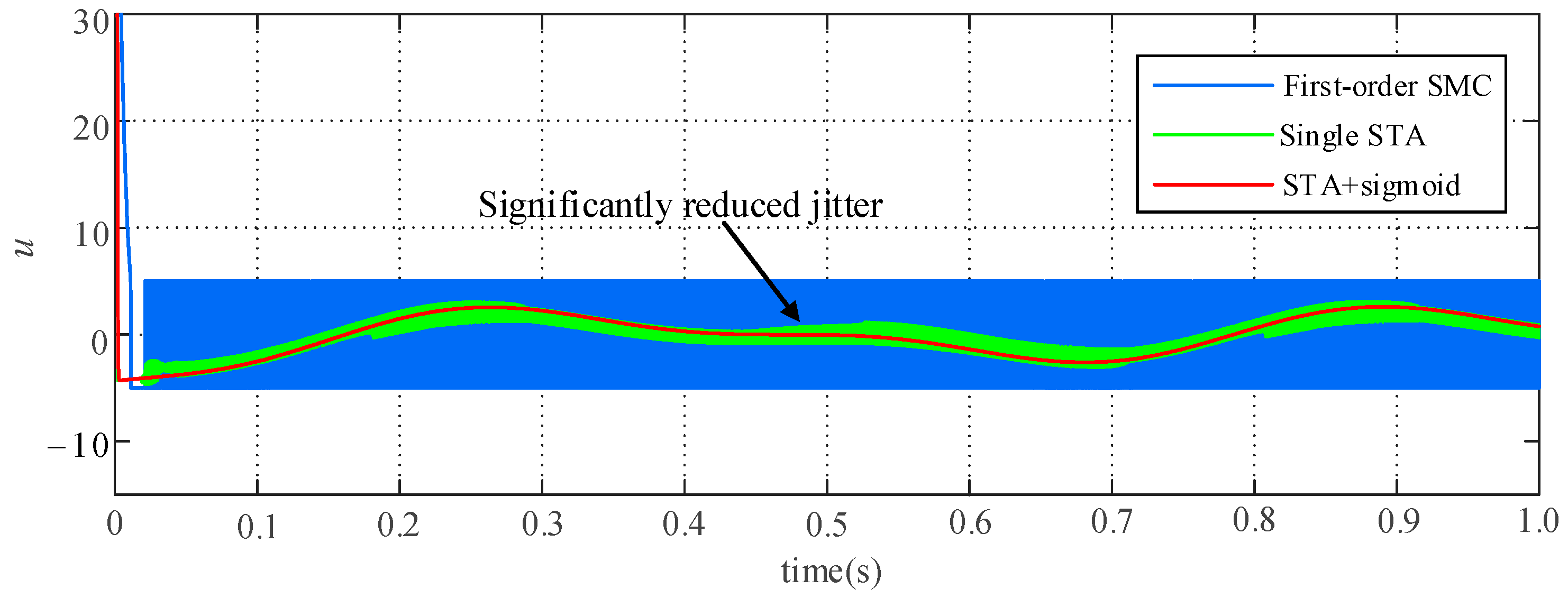
5.1. AQST-SMC Performance Analysis

The simulations of the conventional first-order SMC, conventional STA, and improved AQST-SMC were compared to study the optimization performance of the algorithms and validate the theoretical analyses presented in Section 3. The traditional first-order SMC uses an integral sliding mode surface and the exponential convergence law. In addition, the sign function in the original exponential convergence law is replaced by a saturation function, which is more effective in suppressing jitter (Appendix A). The Pref and Q_ref of port 2 were 0.2 p.u. and 0.3 p.u. At t = 0.02 s, the active and reactive powers of port 2 were assumed to suddenly increase and decrease by 0.2 p.u., respectively. Figure 8 shows the simulation results.

The power response curves presented in Figure 8a,b show that the proposed AQST-SMC method had a faster response speed at the startup moment of the system. Furthermore, it reached a steady state in a shorter time because of the rapid adjustment of convergence when the power changed. Based on the calculations, the power oscillation of the AQST-SMC algorithm using the sigmoid function was considerably smaller in the steady-state operation than in other SMCs. It was approximately 66.71% and 60.13% of the active and reactive oscillations, respectively, under the proposed STA, compared with that under the traditional STA, effectively reducing the power oscillation in the steady-state operation and improving the transient performance of the system.

Table 2. Performance characteristics of FMSSs.

Control Modes	Response Time (ms)	Adjustment Time (ms)	Steady-State Oscillation Amplitude
First-order SMC	P: 4.30	P: 3.95	P: 9.87%
	Q: 5.50	Q: 4.40	Q: 8.91%
Traditional STA	P: 1.00	P: 1.20	P: 6.96%
	Q: 1.23	Q: 1.00	Q: 8.36%
AQST-SMC	P: 0.51	P: 0.32	P: 4.64%
	Q: 0.47	Q: 0.30	Q: 5.03%

lists the output power response time at the system startup moment and the regulation time to return to a steady state when disturbed. Table 2 shows that the active power response times at the startup moment using the proposed AQST-SMC method were 1.96 and 8.43 times those of the traditional STA and first-order SMC algorithm, respectively. The reactive power response times were 2.61 and 11.70 times better than those of the traditional STA and first-order SMC algorithm, respectively. The active power regulation time to return to a steady state when disturbed under the AQST-SMC algorithm improved compared with those of the traditional STA and first-order SMC algorithm. The active power regulation times of the AQST-SMC algorithm were 3.75 and 12.34 times better than those of the traditional STA and first-order SMC algorithm, respectively. Finally, the reactive power regulation times were 3.33 and 14.67 times better than those of the traditional STA and first-order SMC algorithm, respectively. Thus, the proposed AQST-SMC method effectively improved the speed of the system to reach a steady state, and considerably reduced the degree of fluctuation of the system under transient operation. In addition, the robustness and anti-interference capability of the system improved.

5.2. Dynamic Simulation Verification of FMSS System

To further investigate the dynamic performance and anti-interference ability of the control system, this study compared the simulations of several typical working conditions prone to occur under new energy access. The initial operating state of the three-port FMSS is as follows: the output power value of port 1 is Q_1ref = 0 p.u.; the output power values of port 2 are P_2ref = 0.1 p.u. and Q_2ref = 0.3 p.u.; and the output power values of port 3 are P_3ref = 0.2 p.u. and Q_3ref = 0.5 p.u.

Table 3. Parameters of different FMSS controllers.

Control Method	Parameters of Outer Loop Controller	Parameters of Inner Loop Controller
Traditional PI (MMC 1)	kp1 = 0.5, ki1 = 100	kp1 = 22, ki1 = 3.46
Traditional PI (MMC 2)	kp2 = 0.00005, ki2 = 70	kp2 = 22, ki2 = 3.46
Traditional PI (MMC 3)	kp3 = 0.000028, ki3 = 80	kp3 = 22, ki3 = 3.46
First-Order SMC	ε = 1, q = 40, c1 = 30, Δ = 0.05	ε = 3, q = 4000, c1 = 30, Δ = 0.05
AQST-SMC	α1 = 2, β1 = 30, k1 = 10	α1 = 110,000, β1 = 20,000, k1 = 10

lists the parameters of different controllers. The first-order traditional SMC features an additional control action based on the exponential convergence law. Notably, the present study only applied the AQST-SMC in port MMC1 (traditional U_dcQ outer loop) and MMC2, and 3 (traditional PQ control outer loop) used PI control. Furthermore, the controller parameters were calculated and then carefully selected for the optimal steady-state operation of the system, as well as to achieve the desired response speed and convergence.

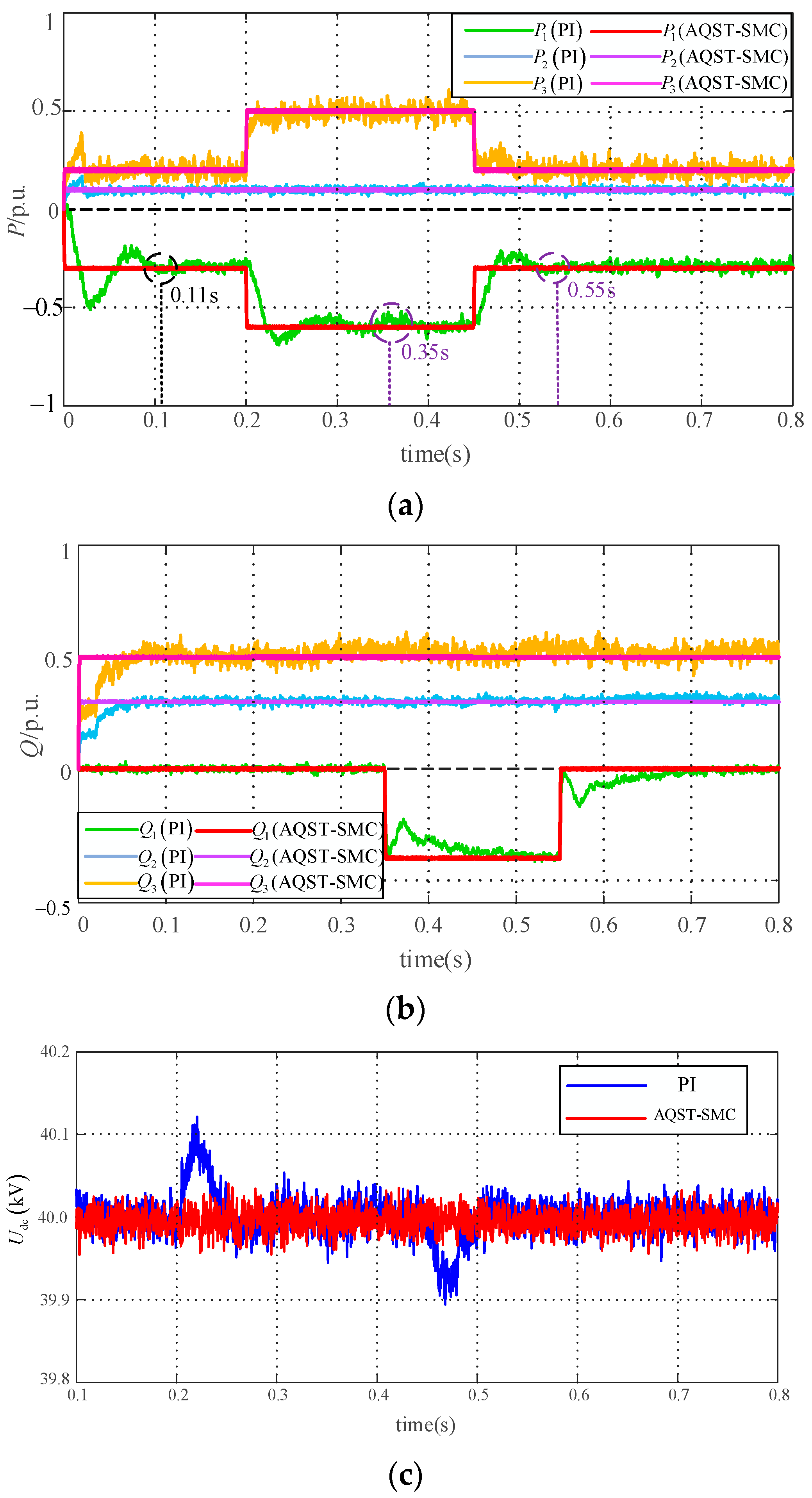
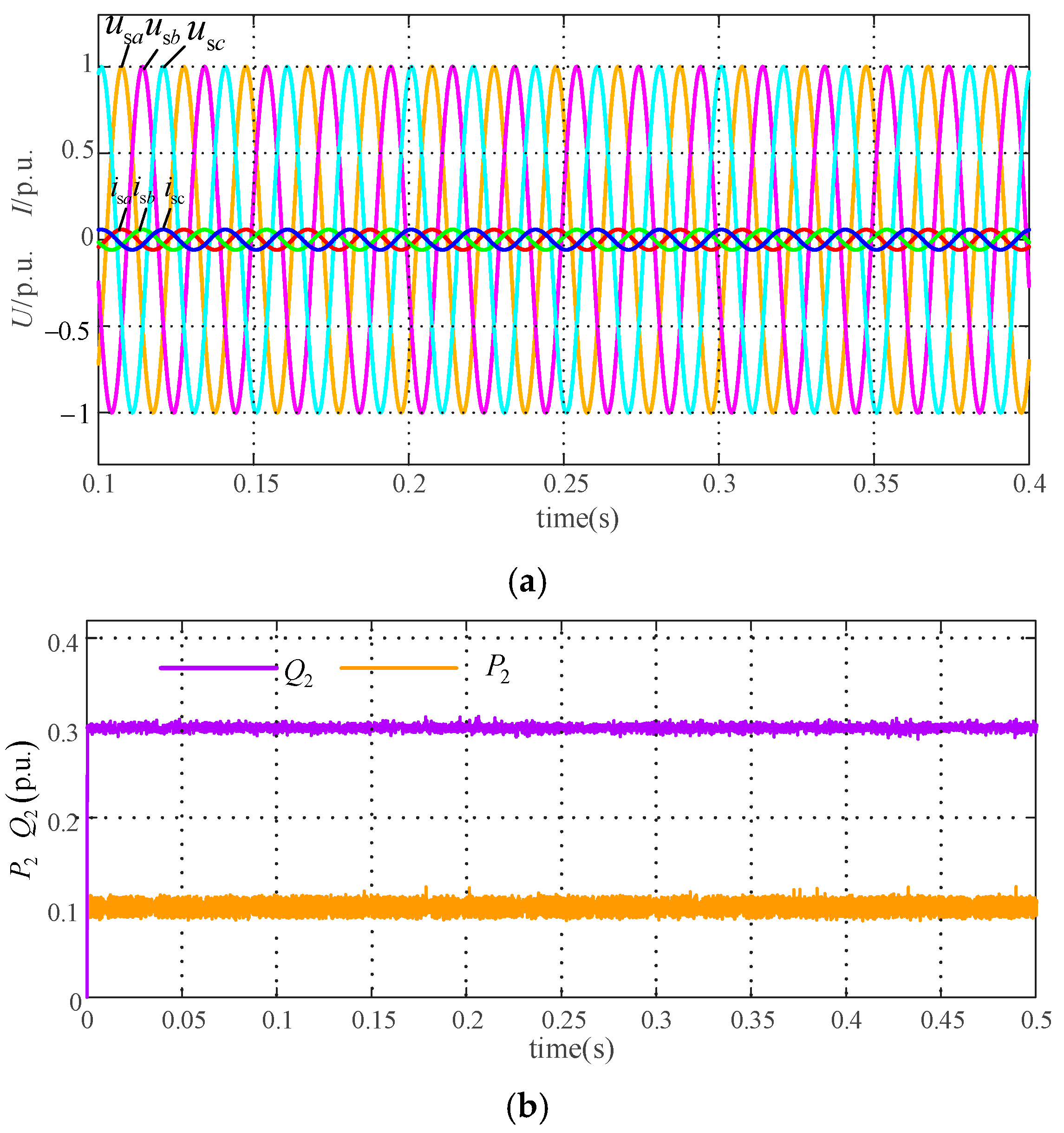
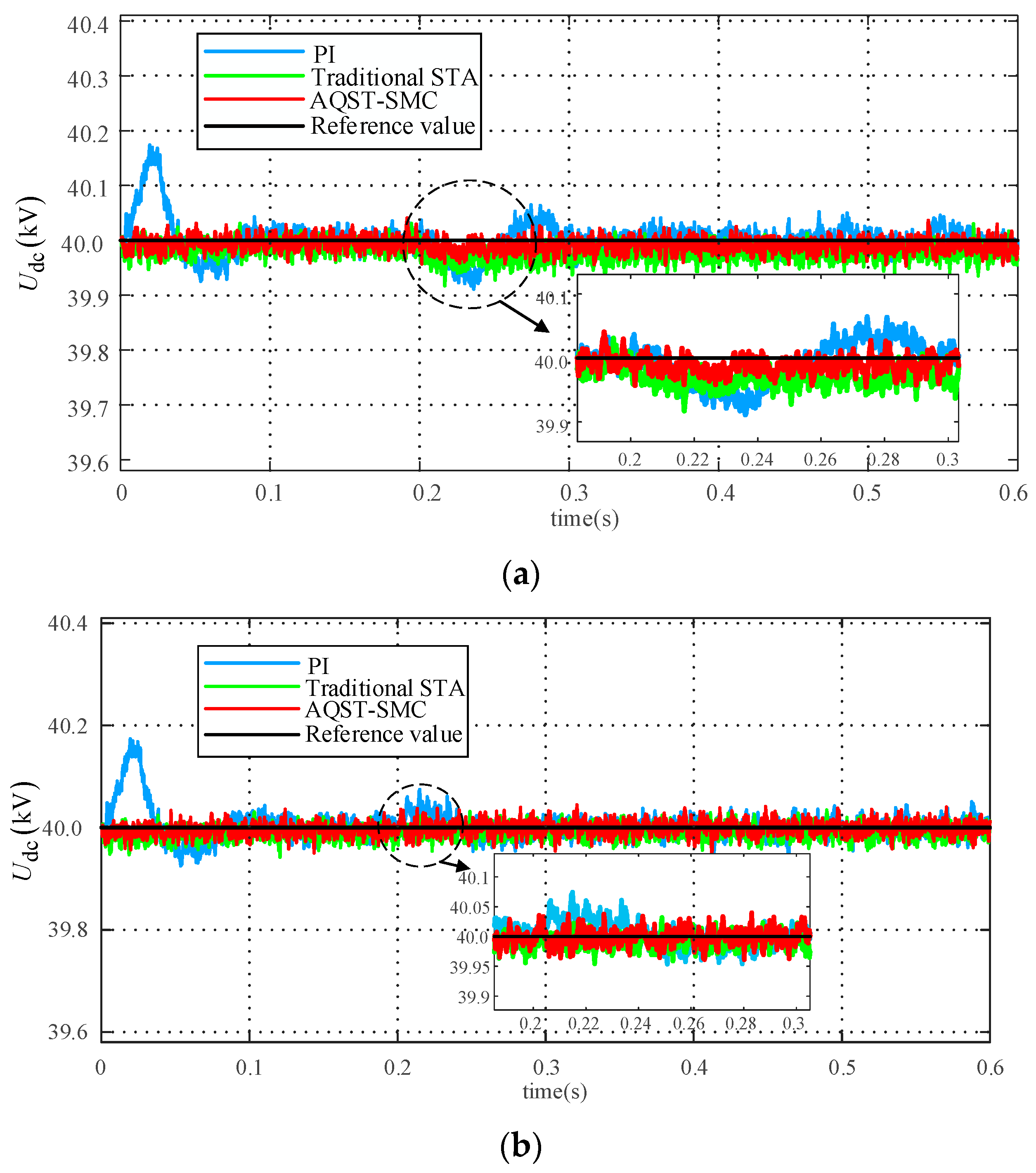
5.2.1. Comparison of Simulations with Disturbed System Output Power

The active power variation affects the stability of the DC-side voltage. The simulation of port 3 was subjected to power fluctuation after accessing distributed power supply and a new type of load. The traditional PI and proposed AQST-SMC algorithm were simulated and compared; Figure 9 shows the output feedback curves of the three-terminal FMSS.

Figure 9 shows that the system startup moment, using the traditional PI control under the output power response, was slow. It took approximately 0.1 s to stabilize. Based on the active power reference of MMC3 at t = 0.2 s, the voltage jumped from 0.2 (standard) to 0.5 to simulate the power fluctuation of the FMSS system caused by the distributed power supply and new load access. Under PI control, the system required approximately 0.12 s to reach a steady state after being perturbed. The dynamic mathematical model of the DC side of the three-port FMSS and the active power balance relationship showed that the active power perturbation affected the stability of the voltage on the DC side [9]; moreover, owing to the inability of the PI controller to adapt to the dynamics of the system under the sudden change of power, the DC voltage fluctuated considerably at 0.2 s and 0.45 s, and the sizes of the oscillations were approximately 112.05 V and 105.85 V, respectively. When the reactive power of MMC1 fluctuated at 0.35 and 0.55 s, its active power suffered from a certain degree of fluctuation, verifying the proposed control strategy for the effectiveness of the power decoupling. Under the proposed AQST-SMC, the system stabilized within 0.001 s at the startup moment and after being disturbed. The dynamic response time was reduced by 100 times, and the DC voltage remained stable. Thus, the feasibility of the AQST-SMC was verified, the anti-disturbance performance of the system considerably improved, the decoupling between the output powers of the system was realized, and the stability of the additive system improved.

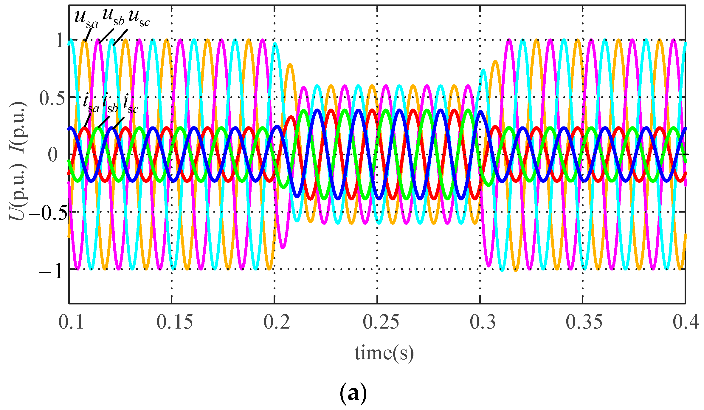
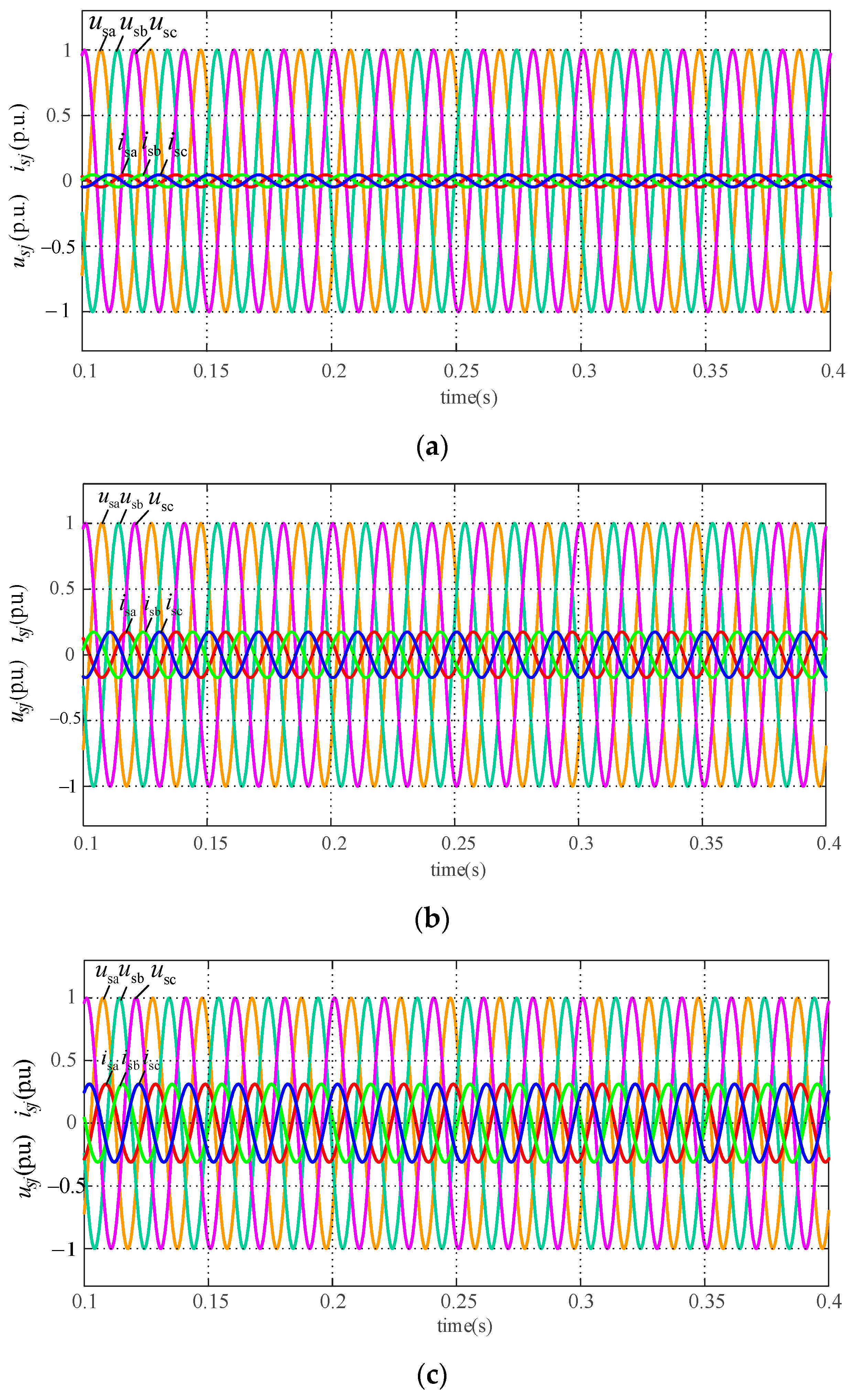
5.2.2. System AC Measured Voltage Amplitude Dips

To validate the proposed method for AC fault measurements, the MMC3 AC voltage was simulated at an amplitude drop of −0.4 (units) in 0.2–0.3 s. Figure 10a shows the AC voltage and current responses; the current response was rapid and accurate. Figure 10b,c show that during voltage dips, the proposed AQST-SMC exhibited good transient characteristics at instances of fault occurrences and good steady-state characteristics during the fault period, compared with the conventional first-order SMC and conventional PI control. The active and reactive powers were rapidly maintained, with fast response and robustness. Figure 11a,b show that during voltage dips at the MMC3 side, MMC2 can function normally without being affected, and its active and reactive powers can remain stable. This indicated that the dynamic response of the system was fast, with good anti-interference properties.

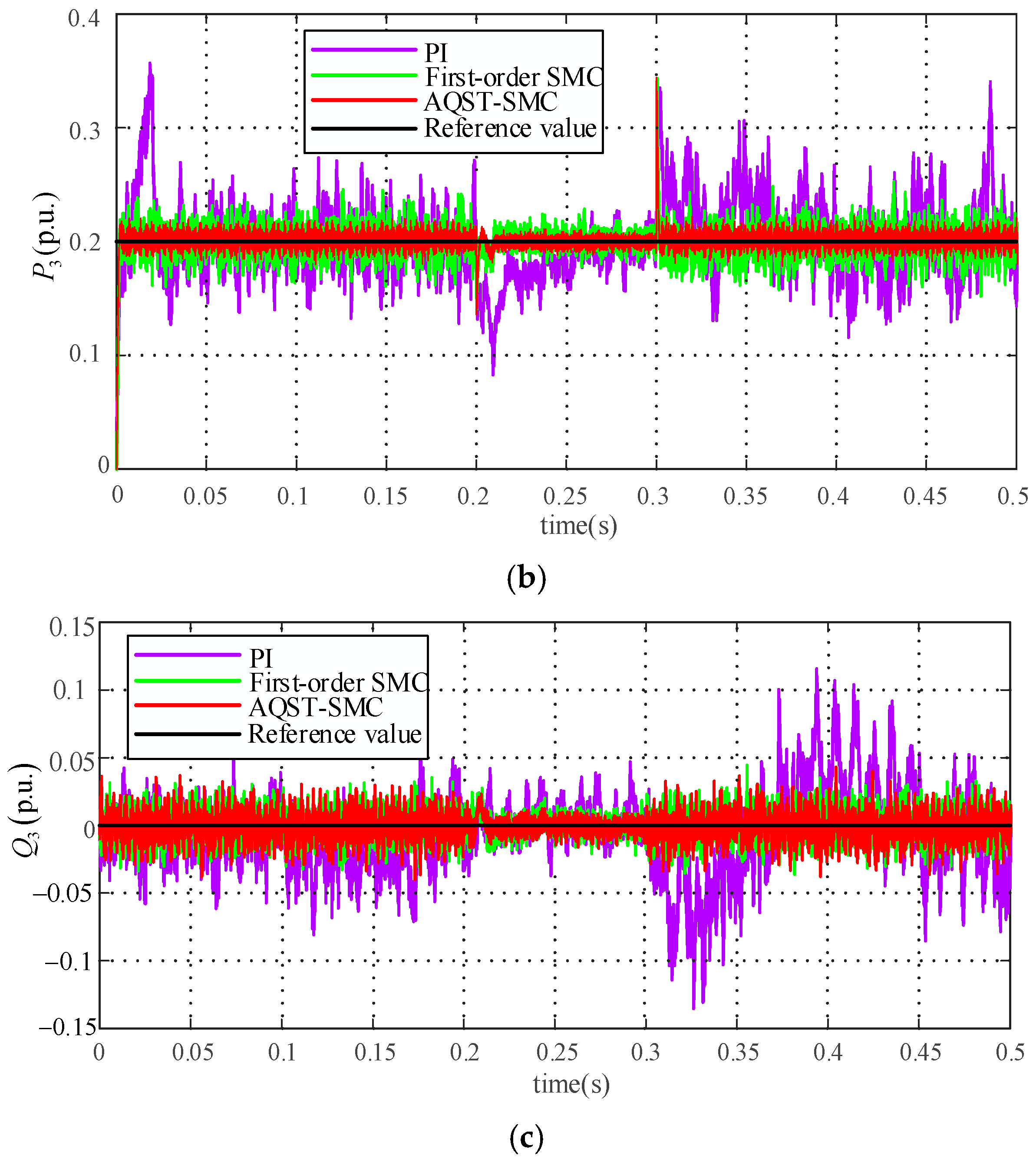
5.2.3. Disturbance of System Electrical Parameters

During practical operation, the AC-side equivalent impedance of the system generated parameter perturbations in response to changes in grid conditions, environmental factors, and load conditions. To analyze the immunity of the system, it was assumed that the AC inductance on the MMC1 side increased to thrice its original value and reduced to 40% of the original value at t = 0.2 s. Figure 12 and Figure 13 show the response curves of the d-axis currents and DC side voltages using the three methods. Under PI control, the system exhibited a slow response at the initial moment, and produced fluctuations in the d-axis currents of approximately 93 A when the inductance parameters were changed. However, the STA and proposed AQST-SMC overcame the problem of slow response at the initial startup moment of the system. The ability of the proposed AQST-SMC to track the reference value of the d-axis current in the steady state and after parameter changes was superior to that of the conventional STA, and the jitter considerably reduced. The DC voltage of the proposed AQST-SMC responded rapidly and fluctuated to a lesser extent at the time of parameter ingestion. Furthermore, the voltage was stabilized at the reference value of 40 kV, confirming the superiority of the AQST-SMC strategy.

5.3. Validation of U_acf Mode of Operation

When the feeder connected to the FMSS fails, to guarantee the operation of important loads, a stable AC voltage and grid frequency must be provided to the power loss area; this is called the U_acf mode of operation. To verify the effectiveness of the AQST-SMC method during power loss, port 2 was set to fail and the load connected at the end was purely resistive (value = 120). Figure 14 shows the three-port AC measurement output response. Figure 14a shows the output voltage and current waveforms of the failed port 2. The output voltage and current were smooth and stable, and the faulty power supply function was realized. Figure 14b,c show that the voltage and current waveforms of ports 1 and 3 remained stable and unaffected by port 2. This confirmed the feasibility of the proposed control strategy, and ensured continuous power supply in the faulty area.

6. Conclusions

This study proposes adaptive super-twisting SMC based on feedback-accurate linearization decoupling for the nonlinear and strongly coupled mathematical model of an FMSS in the distribution network and the difficulty in the traditional PI double-closed-loop control parameter tuning. The main conclusions are as follows:

(1) The three-terminal FMSS nonlinear radiation model was transformed into a linear model via exact feedback linearization and applied to the FMSS inner-loop control design. This completely decoupled the output power, achieved a simple controller design, and improved the operating characteristics of the system.

(2) To address the large jitter vibration and low convergence speed of the first-order SMC, STA control was introduced. AQST-SMC was designed using the sigmoid function and adaptive proportional term to realize better jitter vibration suppression and higher convergence speed, respectively. The inner- and outer-loop composite control system of the FMSS was designed to effectively improve the dynamic response speed, robustness, and steady-state characteristics of the system.

(3) The proposed method improved the transient and steady-state characteristics of the system, with good anti-interference ability under several working conditions with high incidence rates. This can provide insights into innovative solutions for the application of FMSSs in smart distribution networks and new power systems.

Although this study implemented the AQST-SMC algorithm in the U_dcQ and PQ operating modes with the corresponding validation analyses, the dynamic process of switching between different operating modes has not yet been considered. In the future, the different operating conditions of FMSSs should be investigated from the perspective of mode switching. In addition, the proposed AQST-SMC should be applied to the virtual synchronous control of new grid-type energy sources to improve its robustness and response speed.

References

1. Chen, Y.; Tang, Z.; Weng, X.; He, M.; Zhang, G.; Yuan, D.; Jin, T. A novel approach for evaluating power quality in distributed power distribution networks using AHP and S-transform. Energies 2024, 17, 411. [Google Scholar] [CrossRef]
2. Liu, Y.; Hu, J.; Shi, J.; Yang, B. Adaptive integrated control strategy for MMC-MTDC transmission system considering dynamic frequency response and power sharing. J. Electr. Eng. Technol. 2023, 147, 108858. [Google Scholar] [CrossRef]
3. Ivic, D.R.; Stefanov, P.C. An extended control strategy for weakly meshed distribution networks with soft open points and distributed generation. IEEE Access 2021, 9, 137886–137901. [Google Scholar] [CrossRef]
4. Mardanimajd, K.; Karimi, S.; Anvari-Moghaddam, A. Voltage stability improvement in distribution networks by using soft open points. J. Electr. Eng. Technol. 2024, 155, 109582. [Google Scholar] [CrossRef]
5. Li, Z.; Ye, Y.; Wang, Z.; Wu, Y.; Xu, H. Integrated planning and operation evaluation of micro-distribution network based on flexible multistate switch interconnection. CES Trans. Electr. Mach. Syst. 2021, 36, 10. [Google Scholar] [CrossRef]
6. Hou, Y.; Xu, Y.; Wang, Z.; Chen, X.; Cui, H. Research on application of three-port SNOP based on dual closed-loop control in the distribution network. In Proceedings of the IEEE International Conference on Smart Technologies and Management for Computing, Chennai, India, 2–4 August 2017; pp. 389–395. [Google Scholar] [CrossRef]
7. Wang, Z.; Sheng, L.; Huo, Q.; Hao, S. An improved model predictive control method for three-port soft open point. Math. Probl. Eng. 2021, 2021, 9910451. [Google Scholar] [CrossRef]
8. Peng, B.; Zhang, G. Coordination control strategy for three-port SNOP based on FCS-MPC. J. Eng. 2019, 2019, 1005–1010. [Google Scholar] [CrossRef]
9. Aithal, A.; Li, G.; Wu, J.; Yu, J. Performance of an electrical distribution network with soft open point during a grid side AC fault. Appl. Energy 2018, 227, 262–272. [Google Scholar] [CrossRef]
10. Li, Z.; Hao, Q.; Gao, F.; Wu, L.; Guan, M. Nonlinear decoupling control of two-terminal MMC-HVDC based on feedback linearization. IEEE Trans. Power Deliv. 2019, 34, 376–386. [Google Scholar] [CrossRef]
11. Zhang, G.; Tang, B.; Shen, C.; Wang, T.; Xu, C.; Xia, Z. A strategy for suppression of voltage fluctuation on DC side when SOP port is unbalanced. Electr. Meas. Instrum. 2021, 61, 95–101. [Google Scholar] [CrossRef]
12. Li, B.; Liang, Y.; Wang, G.; Li, H.; Ding, J. A control strategy for soft open points based on adaptive voltage droop outer-loop control and sliding mode inner-loop control with feedback linearization. Int. J. Electr. Power Energy Syst. 2020, 122, 106205. [Google Scholar] [CrossRef]
13. Zhou, M.; Su, H.; Zhou, H.; Feng, Y.; Wang, D.; Cheng, J. Full-order sliding mode control strategy for soft open point. Proc. CSEE 2023, 43, 8622–8635. [Google Scholar] [CrossRef]
14. Liu, Y.C.; Laghrouche, S.; Depernet, D.; N’Diaye, A.; Djerdir, A.; Cirrincione, M. Disturbance-observer-based speed control for SPMSM drives using modified super-twisting algorithm and extended state observer. Asian J. Control 2024, 26, 1089–1102. [Google Scholar] [CrossRef]
15. Xu, Q.; Jiang, D.; Wang, Y.; Zhang, X.; Liu, J.; Chen, Y. Variable-step close-loop angle compensation method of PMSM rotor position estimation based on super-twisting sliding-mode observer using tangent reaching law. Energy Rep. 2023, 9, 356–361. [Google Scholar] [CrossRef]
16. Maged, N.A.; Hasanien, H.M.; Ebrahim, E.A.; Tostado-Véliz, M.; Jurado, F. Optimal super twisting sliding mode control strategy for performance improvement of islanded microgrids: Validation and real-time study. Int. J. Electr. Power Energy Syst. 2024, 157, 109849. [Google Scholar] [CrossRef]
17. Ghazi, G.A.; Al-Ammar, E.A.; Hasanien, H.M.; Ko, W.; Lee, S.M.; Turky, R.A.; Tostado-Véliz, M.; Jurado, F. Circle search algorithm-based super twisting sliding mode control for MPPT of different commercial PV modules. IEEE Access 2024, 12, 33109–33128. [Google Scholar] [CrossRef]
18. Saadaoui, A.; Ouassaid, M. Super-twisting sliding mode control approach for battery electric vehicles ultra-fast charger based on Vienna rectifier and three-phase interleaved DC/DC buck converter. J. Energy Storage 2024, 84, 110854. [Google Scholar] [CrossRef]
19. Çelik, D.; Ahmed, H.; Meral, M.E. Kalman filter-based super-twisting sliding mode control of shunt active power filter for electric vehicle charging station applications. IEEE Trans. Power Deliv. 2023, 38, 1097–1107. [Google Scholar] [CrossRef]
20. Tiwary, N.; Naik, N.V.; Panda, A.K.; Narendra, A.; Lenka, R.K. A robust voltage control of DAB converter with super-twisting sliding mode approach. IEEE J. Emerg. Sel. Top. Ind. Electron. 2023, 4, 288–298. [Google Scholar] [CrossRef]
21. Wang, F.; Yang, A.; Yu, X.; Zhang, Z.; Wang, G. Model-free predictive current control for three-phase Vienna rectifier based on adaptive super-twisting sliding mode observer. Trans. China Electrotech. Soc. 2024, 39, 1859–1870. [Google Scholar] [CrossRef]
22. Pati, A.K.; Sahoo, N.C. Adaptive super-twisting sliding mode control for a three-phase single-stage grid-connected differential boost inverter based photovoltaic system. ISA Trans. 2017, 69, 296–306. [Google Scholar] [CrossRef]
23. Hou, J.; Wang, Z.; Zhou, H.; Xu, H.; Wei, W. Soft open point control strategy based on super-twisting-full-order fast terminal composite sliding mode. Autom. Instrum. 2023, 3, 143–147. [Google Scholar] [CrossRef]
24. Wang, Z.; Zhou, H.; Su, H. Disturbance observer-based model predictive super-twisting control for soft open point. Energies 2022, 15, 3657. [Google Scholar] [CrossRef]
25. Ma, W.; Lü, Q.; Zhang, Y.; Zhang, K.; Han, J.; Li, M. Suppression strategy for fault current of flexible multi-state switch in distribution network fault state. Power Syst. Technol. 2021, 45, 4251–4258. [Google Scholar] [CrossRef]
26. Zhang, K.; Wang, L.; Fang, X.; Zhang, K.; Han, J.; Li, M. High-order fast nonsingular terminal sliding mode control of permanent magnet linear motor based on double disturbance observer. IEEE Trans. Ind. Appl. 2022, 58, 3696–3705. [Google Scholar] [CrossRef]
27. Li, P. Convergence of super-twisting algorithm based on quadratic-like Lyapunov function. Control Decis. 2011, 26, 949–952. [Google Scholar] [CrossRef]
28. Levant, A. Sliding order and sliding accuracy in sliding mode control. Int. J. Control 1993, 58, 1247–1263. [Google Scholar] [CrossRef]
29. Yang, H.; Bai, Y.; Chien, Y.R. Generalized super-twisting sliding mode control of permanent magnet synchronous motor based on sinusoidal saturation function. IEICE Electron. Express 2022, 19, 20220066. [Google Scholar] [CrossRef]
30. Fu, K.; Yi, H.; Zhuo, F.; Li, S. Self-healing control strategy based on snop under severe fault condition. In Proceedings of the 2021 IEEE Sustainable Power and Energy Conference (iSPEC), Nanjing, China, 23–25 December 2021. [Google Scholar] [CrossRef]
31. Li, X.; Liu, J.; Yin, Y.; Zhao, K. Improved super-twisting non-singular fast terminal sliding mode control of interior permanent magnet synchronous motor considering time-varying disturbance of the system. IEEE Access 2023, 11, 17485–17496. [Google Scholar] [CrossRef]
32. Tripathi, V.K.; Kamath, A.K.; Behera, L.; Verma, N.K.; Nahavandi, S. Finite-time super twisting sliding mode controller based on higher-order sliding mode observer for real-time trajectory tracking of a quadrotor. IET Control Theor. Appl. 2020, 14, 2359–2371. [Google Scholar] [CrossRef]
Figure 1. Structure diagram of three-terminal FMSS system.
Energies 17 02643 g001
Figure 2. STA phase plane trajectory.
Energies 17 02643 g002
Figure 3. Symbolic and sigmoid functions for different values of n.
Energies 17 02643 g003
Figure 4. Comparison of the effect of different sliding mode control laws to converge to s = 0.
Energies 17 02643 g004
Figure 5. Comparison of vibration suppression effects of different sliding mode control laws.
Energies 17 02643 g005
Figure 6. Voltage outer loop AQST-SMC block diagram.
Energies 17 02643 g006
Figure 7. Block diagram of three-terminal FMSS AQST-SMC control strategy.
Energies 17 02643 g007
Figure 8. Power response characteristics of port 2. (a) Active and (b) reactive power characteristic curves.
Energies 17 02643 g008
Figure 9. Output feedback of FMSS system under power perturbations. (a) Active power, (b) reactive power, and (c) DC voltage response curves.
Energies 17 02643 g009
Figure 10. MMC3 output feedback under voltage drop. (a) MMC3 voltage and current. (b) MMC3 active power. (c) MMC3 reactive power.
Energies 17 02643 g010aEnergies 17 02643 g010b
Figure 11. MMC2 output feedback under voltage drop. (a) MMC2 voltage and current. (b) MMC2 active and reactive power.
Energies 17 02643 g011
Figure 12. Current response of phase a of MMC1 under parameter perturbation. (a) L tripled. (b) L reduced to 40% of the original value.
Energies 17 02643 g012
Figure 13. DC voltage response under parameter perturbation. (a) L tripled. (b) L reduced to 40% of the original value.
Energies 17 02643 g013
Figure 14. AC side response of ports in the Uacf mode. Voltage and current of ports (a) 2, (b) 1, and (c) 3.
Energies 17 02643 g014