Optimization and Modeling of a Dual-Chamber Microbial Fuel Cell (DCMFC) for Industrial Wastewater Treatment: A Box–Behnken Design Approach

Abstract

Microbial fuel cells (MFCs) have garnered significant attention due to their capacity to generate electricity using renewable and carbon-neutral energy sources such as wastewater. Extensive experimental work and modeling techniques have been employed to dissect these processes and understand their respective impacts on electricity generation. The driving force is to enhance MFC performance for practical applications commercially. Among the various statistical modeling approaches, one particularly robust tool is the Design of Experiments (DoE). It serves to establish the relationships between different variables that influence MFC performance and allows for the optimization of the MFC configuration and operation for scaled-up performances in terms of bioelectricity generation. This study focused on optimizing microbial fuel cells (MFCs) for bioelectricity production using industrial wastewater treatment, employing the Box–Behnken design (BBD) methodology. Through an analysis of response surface models and ANOVA tests, it was found that a combined approach of reduced quadratic, reduced two-factor interaction, and linear models yielded sound results, particularly in voltage yield, COD removal, and current density. Second-order regression models predicted optimal conditions for various parameters, with surface area, temperature, and catholyte dosage identified as critical input variables for optimization. Under these conditions, conducted by the four-factor and three-level Box–Behnken design methodology in a double-chamber MFC unit considering eight output variables—CCV yield, % COD removal, current density, power density, % TSS removal, % CE, and % ${\mathrm{P}\mathrm{O}}_4^{3-}$—the optimum values were 700 mV, 54.4%, 54.4 mA/m², 73.7 mW/m², 99%, 21.2%, and 100%, respectively. At optimum operating conditions, the results revealed a desirability of 76.6% out of a total of 92 iterations. The paper highlights the effectiveness of statistical ANOVA fit-statistics modeling and optimization in enhancing DCMFC performance, recommending its use as a sustainable bioenergy source. Furthermore, validation results supported the above optimization output response findings and confirmed the viability of biorefinery wastewater as an anolyte for scaling up DCMFC bioelectricity generation.

1. Introduction

Microbial fuel cells (MFCs) are intricate systems that blend biological and electrochemical processes simultaneously, posing challenges when it comes to optimizing their performance [1]. Employing statistical experimental design techniques to fine-tune MFC operating conditions holds the promise of yielding more precise responses in line with the desired objectives [1]. Utilizing the Design of Experiments (DoE) approach not only helps extract substantial information but also trims the cost and time required for conducting experiments. This paper focuses on one of the widely used experimental design techniques for screening and optimizing factors in MFC-related research. It was observed that Response Surface Methodology (RSM) proves valuable in describing and optimizing complex nonlinear systems such as MFCs. However, selecting the appropriate experimental design method primarily hinges on the study’s goals, the number of variables in play, the potential for interactions, and the available resources. When it comes to choosing which factors to investigate in depth, simple factorial plans can be a starting point [2,3]. However, to achieve the best possible parameter settings, more intricate designs are often necessary. Among these, Response Surface Methodology (RSM) stands out as a widely favored approach [1]. Various optimization designs are at researchers’ disposal, including full-factorial, response surface (such as central composite and Box–Behnken designs), optimal, and mixture designs (like simplex lattice and simplex centroid designs) [4,5,6,7,8,9,10,11,12,13].

The outcomes of Design of Experiments (DoE) studies undergo rigorous analysis to pinpoint the factors that exert statistically significant influence on the response, as well as to unveil potential interdependencies among them [1]. Various tools and techniques come into play for these analyses, including the use of half-normal plots, Analyses of Variance (ANOVAs), and other methods [1,14,15,16,17]. To illustrate the nonlinear trends in the data, contour plots and Response Surface Methodology (RSM) are often employed. Conducting and analyzing DoE experiments is made feasible through specialized statistical software. Some well-known commercial packages for this purpose encompass Minitab, Statistica, SPSS, SAS, Design-Expert, Stat-graphics, Prisma, MODDE, DoE Fusion PRO, STAVEX, and more. Engaging in any DoE experiment necessitates a grasp of statistical methods such as ANOVA and linear regression, as these are foundational in the process [4,5,7,12,18,19,20,21,22,23,24,25,26,27].

Screening designs primarily elicit linear responses, which may not account for the curvature in the response. To analyze this curvature in the response, researchers often employ quadratic response surface modeling. The Box–Behnken design (BBD) stands out as an independent quadratic response surface design that does not encompass an embedded factorial or fractional factorial design [1,14]. This design necessitates three levels for each factor and generates fewer experimental runs compared to the central composite design when considering the same number of factors [1,14,28]. While the treatment combinations in the BBD are located at the midpoints of the experimental domain’s corners and at the center, a central composite design includes experimental trials where all factors are set at their extreme values [5]. The BBD is a cost-effective alternative to the central composite design but may not be suitable for sequential experiments. It provides robust coefficient estimates toward the center of the design space but weaker ones toward the design space’s edge [29,30,31]. Several studies have utilized the BBD for optimization, as shown in

Table 1. A concise overview of the applications and key findings of each study that employed the Box–Behnken design (BBD) for optimization in various microbial fuel cell (MFC) applications [1,30,31].

Study	Application	Design	Findings
[32]	Optimization of cathodic parameters	BBD (Three-factor, three-level)	The cathode surface area was found to be the most significant parameter in MFC performance.
[33]	Factors affecting continuous-flow BER-MFC	BBD (Three-factor, three-level)	The order of significance: COD load > HRT > nitrate load.
[34]	Maximizing power density in dual-chamber MFC	BBD (Four-factor, three-level)	Temperature and external resistance were identified as significant parameters.
[35]	Pyraclostrobin elimination in MFC–Fenton	BBD (Three-factor, three-level)	Catholyte pH significantly affected Fenton reaction performance.
[36]	Dual-chamber MFC performance evaluation	BBD (Four-factor, three-level)	pH and inoculum composition interactions impacted MFC performance.
[37,38,39]	Influence of glucose concentration on MFC	BBD (Three-factor, three-level)	High OCV was obtained at a high glucose/yeast ratio and low glucose concentration.
[32,35,36,37,40,41,42]	Oxyfluorfen degradation in dual-chamber MFC	BBD (Three-factor, three-level)	Optimal conditions of temperature, pH, and initial oxyfluorfen concentration were identified.
[43]	Effect of operating parameters on ceramic MFC	BBD (Three-factor, three-level)	Optimum conditions for maximizing power output were established.

.

These studies leveraged the BBD to conduct experiments and optimize various parameters, demonstrating its applicability and effectiveness in different MFC-related investigations. However, it is important to note that the predictability of this design may be compromised as it does not include a treatment combination where all factors are at their boundary values simultaneously. This study’s primary purpose and knowledge contribution involved optimizing the MFC scaling-up factors, particularly, fine-tuning towards optimum operating temperature, electrode surface area (bi-electrode configurations), HRT, and the catholyte dosage concentration, which is often linked to improved overall power output (closed-circuit voltage yield) in the DCFMC unit once perfectly optimized. The study recognized the need for practical and robust DCMFC designs with the potential of applicability in real-world, industrial settings while overcoming limitations such as in the cell overall voltage (CCV—mV) and lower or impractical Faraday/coulombic efficiencies (% CE). To achieve this, this paper emphasizes the importance of validating laboratory-scale results through lab-scale/benchtop and further computational applications to assess the long-term performance and possibilities of sustained scaling-up design methodology and, perhaps, the potential prospects of the grid connection of this technology to the nation power grid as an alternative power source. This validation process is crucial for identifying potential issues early on and ensuring the reliability of the DCMFC RSM–BBD methodology towards scaling up bioelectricity generation.

The novelty and new knowledge contribution of this paper lie in several key aspects. Our study represents a novel application of Response Surface Methodology (RSM) in conjunction with microbial fuel cells (MFCs) for optimizing bioelectricity generation while treating industrial wastewater. This application of statistical modeling provides a systematic approach to optimizing MFC performance, which is innovative in the field. The study employed the four-factor, three-level Box–Behnken design (BBD) method to optimize factors affecting the DCMFC performance: temperature, hydraulic retention time (HRT), surface area, and catholyte dosage. The three level midpoints of the experimental domain relate to 13 experimental combinations that were predicted for the optimization of the four scaling-up factors in this study. This methodology allowed for a comprehensive exploration of optimal operating conditions, contributing to the advancement of DCMFC optimization techniques. The study considered multiple response output variables including closed-circuit voltage (CCV) yield, % COD removed, maximum current density, optimum power density, Faraday/coulombic efficiency (% CE), % TSS removal, % TOC removal, and % ${\mathrm{P}\mathrm{O}}_4^{3-}$ removal. This comprehensive evaluation provided valuable insights into the overall performance of the MFC system and its potential for bioelectricity generation. Rigorous validation via ANOVA tests and regression models ensured the accuracy and reliability of the study’s findings. The identification of optimal operating conditions for the DCMFCs, in variables such as the specific surface area, temperature, and catholyte dosage, represents a significant contribution to the field by providing practical insights for improving MFC performance.

The paper highlights the practical applicability of DCMFCs as a sustainable and renewable bioenergy solution, particularly in addressing energy challenges faced in regions like South Africa, as reported by Shabangu et al. [44,45], by recommending the potential of DCMFC technology for national grid connections, which is further investigated computationally for potential DCMFC inverter modeling and potential applications. This paper generally offers valuable insights into promoting sustainability in energy production. The paper examines the novelty of the BBD optimization methodology in achieving the practicality and applicability of DCMFC findings for the purpose of upscaling and commercializing DCMFC technology. The experimental results of this paper demonstrate a high degree of transferability. Several novel practices highlight the potential for industrial-scale applications:

• The utilization of raw industrial wastewater sources harvested from local wastewater treatment plants, effectively emulating the complexity and variability of industrial wastewater substrates based on day-to-day industrial activities.
• The employment of freshly harvested and well-acclimatized heterotrophic biomass consortia, specifically Protobacteria and Bacteriodota, as a combined biomass population to enhance biodegradability in the microbial fuel cell.

These aspects underscore the practical transferability of this study’s findings to industrial applications. The paper highlights the novelty of the BBD methodology for optimizing DCMFCs, particularly demonstrating its capacity for reliable laboratory-scale factor interactions. While practical application may present complexities that could limit the smooth implementation of the BBD approach used here, the paper convincingly demonstrates the treatment capacity and bioelectrochemical potential of this technology. Overall, the paper’s novel approach to optimizing the DCMFC bioelectricity generation capacity using statistical modeling, combined with its comprehensive evaluation of response variables and potential practical implications for sustainability, represents a significant contribution to the field of bioenergy research.

2. Results and Discussion

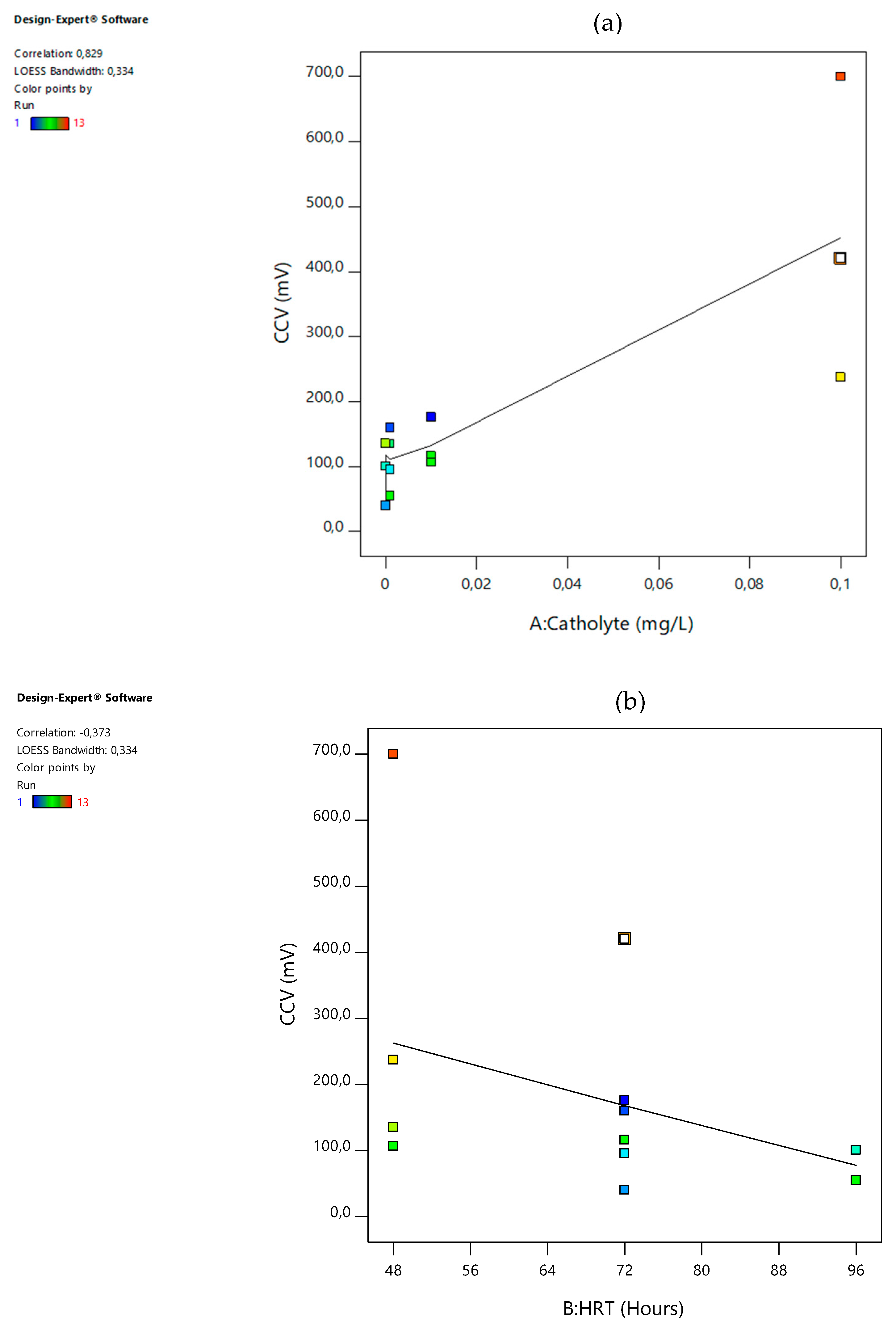
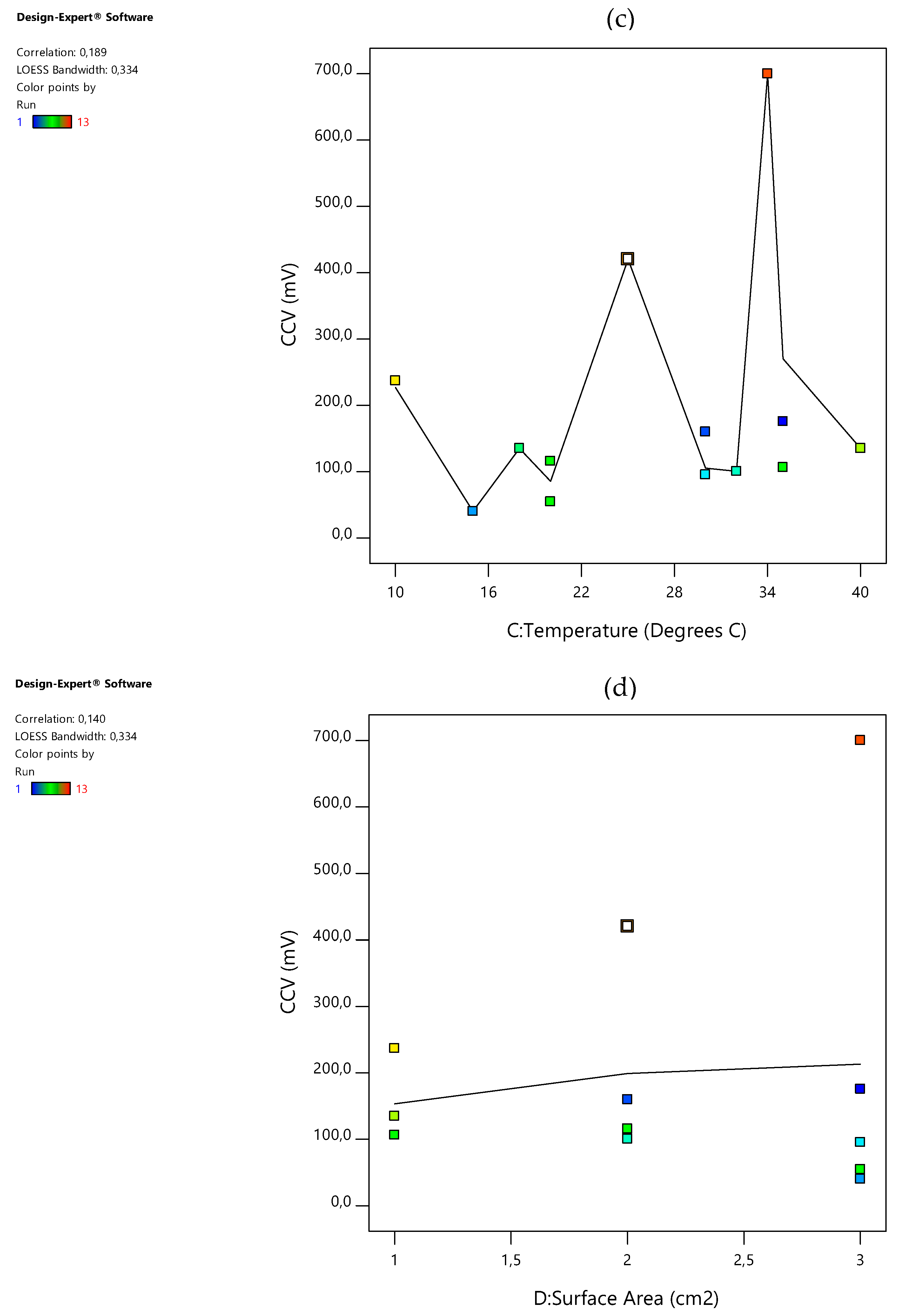
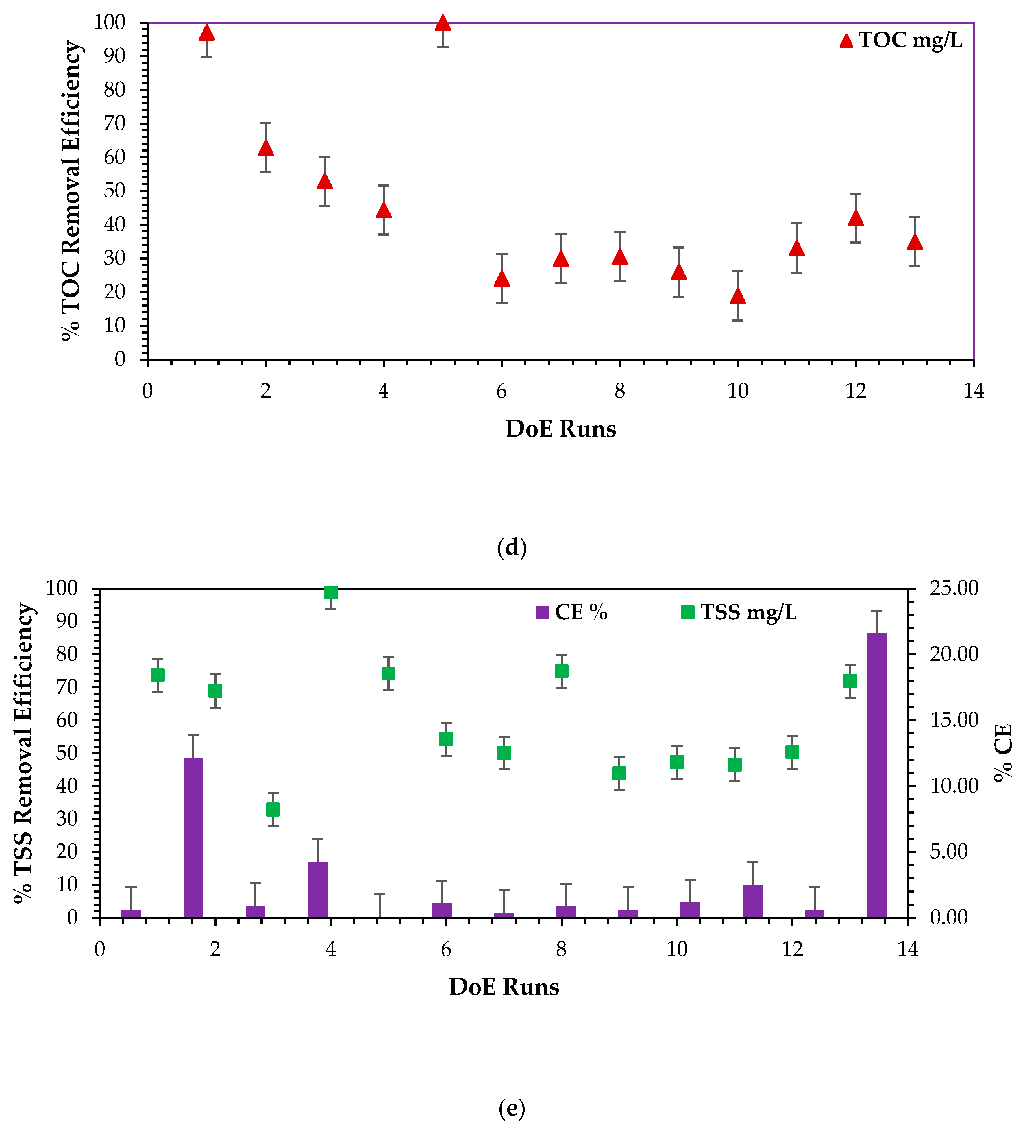
2.1. Influence of Input Variables on the Responses

A scatter plot graph is a significant plot in statistical analysis as it measures the effect of each process variable on the output response. With each process, variables compromising the coded values versus the output response are presented in Figure 1a–d below. The relationship between the process variables and the output response was initially assumed to constitute a linear model. Hence, the gradient of the plots may be used to represent the correlation. This correlation, once assumed positive, signifies that a direct proportionality exists between the process variable and the response output whereas a negative correlation presents an indirectly proportional response output from the process; see the correlations for temperature, catholyte dosage, and electrode surface area and hydraulic retention time (HRT) or incubation time. Hence, in this study, increasing either one of the basic operating factors resulted in an increase in the closed-circuit voltage (CCV) alternative-energy generation. The increasing order of the absolute values of correlations revealed the following observations: surface area had a correlation value of 0.140 at the 3-CCu bi-electrode, temperature had a correlation value of 0.189 at 34 °C, HRT had a correlation factor of 0.373 at 48 h, and catholyte had a correlation of 0.829 at 0.1 mol/L. Similarly, % COD removal, % total phosphate (${\mathrm{P}\mathrm{O}}_4^{3-}$) removal, current density (ID), power density (PD), % TSS removal, % TOC removal, and % CE were all producing the same positive outcomes. Moreso, these findings present a good basis for statistical analysis. The assumption made while preparing this section was that the data points resembled a linear model; however, the correlation of the temperature, HRT, and surface area factor clearly produced, rather, a very low correlation significance with respect to the closed-circuit voltage (CCV) generation yield in the DCMFC unit. Furthermore, a clearly strong, statistically highly significant correlation between the catholyte concentration and potassium permanganate dosage concentration emerged as very influential to the scaled-up production of bioelectricity in the DCMFC with correlation factors ≥ 0.83, as shown in Figure 1d. This correlation is therefore considered the DCMFC scaling-up design factor and shall be further discussed in the following sections of this paper in terms of its impact on the DCMFC’s ability to produce a commercial-scale voltage yield and reasonable Faraday/coulombic efficiencies approaching the 50% mark.

2.2. Regression Model and Fit Summary

Response transformation is an essential technique in data analysis. In statistical analysis, response power transformation involves applying various mathematical functions to the responses. The mathematical functions evaluated using the design expert software for transformation included the following: no. of transformation, natural log, inverse square root, square root, base 10 logarithm, logit, inverse, arcsine square root, and power transformation. The transformations for CCV, power density, current density, % TOC removed, % TSS removed, % COD removed, % total phosphates removed (${\mathrm{P}\mathrm{O}}_4^{3-}$), and % CE were as shown in detail in Tables S5–S12 in the Supplementary Materials section. With no transformation required for the responses, the subsequent step involves determining the appropriate types of models. The Design Expert software offers several valuable statistical tables to aid in identifying the suitable model for detailed analysis. A critical table for model selection in statistical analysis is the fit summary table. This section consolidates the significant statistical parameters necessary for choosing the starting point for the actual model. Tables show fit summaries for temperature (X₁), electrode surface area (X₂), catholyte concentration (X₃), and hydraulic residence time (X₄) with regard to the generation of voltage yield–closed-circuit voltage (Y₁), power density (Y₂), current density (Y₃), coulombic efficiency (CE%) (Y₄), Chemical Oxygen Demand (COD) (Y₅), total phosphates (${\mathrm{P}\mathrm{O}}_4^{3-}$) (Y₆), total suspended solids (TSS) (Y₇), and total organic carbon (TOC) (Y₈).

The linear, cubic, two-factor interaction (2FI) model and quadratic model were the types of models that were investigated. In statistical analysis, the model with the highest sequential p-value, F-value, and adjusted R² is regarded as the model that will best fit the data points (Stat-Ease Inc., 2021). For all responses, the linear model had the highest sequential p-value and adjusted R² values. On the other hand, the two-factor interaction (2FI) had the second most reliable sequential p-value and adjusted R² values. Therefore, these results suggested that the best-fitting model was either the linear model or the two-factor interaction (2FI) model. Notably, the quadratic model was aliased since there were no sufficient unique design points to predict all coefficients of the model. This model was the last wherein least-squares estimations would not be unique, resulting in 3D plots with shapes that had recurrent plateaus, which depict erroneous statistical analysis from a statistical viewpoint. Based on the above digressed reasons, the linear model was suggested for the optimization investigation of the DCMFC unit in this study, motivated by the optimization findings suggesting that most statistically significant values were of the linear-model type, suggesting the highest statistical significance in this investigative study.

2.3. Analysis of Variance (ANOVA) Test and Fit Statistics

The analysis of variance (ANOVA) test is one of most significant tests in statistical analysis. The ANOVA test helps a researcher observe the selected effects and the coefficients of a model (reference). Tables S13 and S20 in the Supplementary Materials section define ANOVA response outputs for voltage yield—closed-circuit voltage (Y₁), power density (Y₂), current density (Y₃), coulombic efficiency (% CE) (Y₄), Chemical Oxygen Demand (COD) (Y₅), total phosphates (${\mathrm{P}\mathrm{O}}_4^{3-}$), (Y₆), total suspended solids (TSS) (Y₇), and total organic carbon (TOC)(Y₈). The F-value, probability ≥ F, coefficient of determination (R²), and lack of fit are critical statistical values that assess how well the chosen regression model fits the experimental data points [1,14,15,28,35,46,47]. The F-test determines the significance of the differences between the means of the operating conditions. F-values of 47, 49, 87, 65, 96, 51, 5.52, 4112.7, 5.8, 5.54, and 6.11 indicated that the regression models were significant for closed-circuit voltage.

Another crucial statistical parameter is the p-value, which is closely associated with the F-value. In statistical analysis, the p-value indicates the probability of the regression model being valid [1,35]. As shown in the ANOVA Tables S13–S20 in the Supplementary Materials section, p-values were less than 0.001 for closed-circuit voltage (CCV), % COD removal, current and power densities, phosphates $\left({\mathrm{P}\mathrm{O}}_4^{3-}\right)$, total suspended solids (TSS), and total organic carbon (TOC). The null hypothesis should be rejected if the p-value is significantly small, i.e., less than the alpha value (α) [1,35]. The investigation was conducted at a 95% confidence interval (CI), so the alpha value was 100-CI = 5%. A p-value below 0.05 is considered significant while a p-value greater than 0.1 is considered non-significant and can be ignored.

For CCV yield and the other parameters, the p-values for the terms AB, AD, BC, BD, and A² were below 0.05, indicating that these model terms have significant effects when included in the models. Additionally, the p-value below 0.05 for the power-density term A signified its significance in the model. Values greater than 0.1000 indicate that a model’s terms are not significant. Current density also displayed a significant A model value below the 0.05 threshold. The % COD removal presented B, D, BD, and D² as significant model terms. Total phosphate removal capacity also displayed a case of B, C, D, AB, AD, BC, BD, CD, and B² being significant model terms. Furthermore, the p-value below 0.05 for coulombic efficiency (% CE) was A, indicating that the model term was significant. The % TSS removal once again presented a case of B, C, AB, AD, and C² being significant model terms. These above listed p-values were less than 0.0500, indicating that the model terms were significant. Values greater than 0.1000 indicate that a model’s terms are not significant. If there are many insignificant model terms (not counting those required to support hierarchy), model reduction may improve the overall model outcome.

An equation, formulated in terms of coded factors, enables predictions regarding the response for specific levels of each factor. High levels of factors are coded as +1 while low levels are coded as −1 by default. This coded equation serves to highlight the relative impact of factors by comparing their coefficients. Each coefficient estimate signifies the expected change in response per unit change in factor value, assuming all other factors remain constant. In an orthogonal design, the intercept represents the overall average response across all runs, with coefficients serving as adjustments around this average based on factor settings. When factors are orthogonal, the Variance Inflation Factors (VIFs) equal 1; VIFs exceeding 1 indicate multicollinearity, with higher VIFs suggesting more pronounced factor correlation. Generally, VIFs below 10 are deemed tolerable. The model equations for the anticipated output response at optimal operating factor conditions are as follows:

CCV = 181.54 + 143.49 × A + 0.655 × B + 7.61 × C + 54.07 × D − 1.35 × AB + 96.34 × AD − 67.34 × BC −
37.03 × BD + 77.33 × CD + 95.75 × A²

PD = 13.51 + 12.51 × A − 7.44 × B − 3.15 × C + 19.77 × D − 7.04 × AB − 4.23 × AC + 20.62 × AD + 2.40
× BC + 0.432 × BD − 1.59 × CD

ID = 23.00 + 11.75 × A − 2.10 × B − 15.86 × C + 14.55 × D − 1.24 × AB − 17.49 × AC + 20.76 × AD − 1.19 × C −
57.48 × D − 48.18 × BD + 59.06 × D²

COD = 38.79 + 8.17 × A − 60.83 × B + 1.19 × C − 57.48 × D − 48.18 × BD + 59.06 × D²

$$\begin{gathered} {\mathrm{P}\mathrm{O}}_4^{3-}= 55.72 - 0.423 \times A - 66.50 \times B + 35.59 \times C + 77.74 \times D - 69.21 \times AB + 55.04 \times AD + 66.41 \times BC + \\ 109.50 \times BD - 39.88 \times CD - 66.16 \times B^2 - 42.00 \times D^2 \end{gathered}$$

CE = 0.151 + 0.0515 × A − 0.448 × B − 0.110 × C + 0.242 × D − 0.204 × BC − 0.904 × BD + 0.729 × B²

TSS = 61.94 − 12.66 × A − 36.07 × B + 36.21 × C − 12.79 × D − 24.29 × AB − 23.72 × AD − 63.68 × C²

TOC = 44.87 + 1.43 × A − 0.998 × B + 48.28 × C + 18.79 × D + 75.54 × BC − 24.73 × CD

An equation in terms of actual factors can be used to make predictions about the response for given levels of each factor. These equations can be presented in the following sequence:

CCV = 181.54 + 143.49 × (catholyte) + 0.655 × (HRT) + 7.61 × (temperature) + 54.07 × (surface area) − 1.35 × (catholyte) ×
(HRT) + 96.34 × (catholyte) × (surface area) − 67.34 × (HRT) × (temperature) − 37.03 × (HRT) × (surface area) + 77.33 ×
(temperature) × (surface area) ₊ 95.75 × (catholyte)²

PD = 13.51 + 12.51 × (catholyte) − 7.44 × (HRT) − 3.15 × (temperature) + 19.77 × (surface area) − 7.04 × (catholyte) ×
(HRT) − 4.23 × (catholyte) × (temperature) + 20.62 × (catholyte) × (surface area) + 2.40 × (HRT) × (temperature) + 0.432 ×
(HRT) × (surface area) − 1.59 × (temperature) × (surface area)

ID = 23.00 + 11.75 × (catholyte) − 2.10 × (HRT) − 15.86 × (temperature) + 14.55 × (surface area) − 1.24 × (catholyte) ×
(HRT) − 17.49 × (catholyte) × (temperature) + 20.76 × (catholyte) × (surface area) − 1.19 × (temperature) − 57.48 ×
(surface area) − 48.18 × (HRT) × (surface area) + 59.06 × (surface area)²

COD = 38.79 + 8.17 × (catholyte) + 60.83 × (HRT) + 1.19 × (temperature) − 57.48 × (surface area) − 48.18 × (HRT) ×
(surface area) + 59.06 × (surface area)²

$$\begin{gathered} {\mathrm{P}\mathrm{O}}_4^{3-} =55.72-0.423\times \left(catholyte\right)-66.50\times \left(HRT\right)+35.59\times \left(temperature\right)+77.74\times (surface area)-69.21\times \\ \left(catholyte\right)\times \left(HRT\right)+55.04\times \left(catholyte\right)\times (surface area)+66.41\times \left(HRT\right)\times \left(temperature\right)+109.50\times \left(HRT\right)\times (surface area)-39.88 \\ \times \left(temperature\right)\times (surface area)-66.16\times {\left(HRT\right)}^2-42.00\times {(surface area)}^2 \end{gathered}$$

CE = 0.151 + 0.0515 × (catholyte)− 0.448 × (HRT) − 0.110 × (temperature) + 0.242 × (surface area) − 0.204 × (HRT) ×
(temperature) − 0.904 × (HRT) × (surface area) + 0.729 × (HRT)²

TSS = 61.94 − 12.66 × (catholyte) − 36.07 × (HRT) + 36.21 × (temperature) − 12.79 × (surface area) − 24.29 × (catholyte) ×
(HRT) − 23.72 × (catholyte) × (surface area) − 63.68 × (temperature)²

TOC =44.87 + 1.43 × (catholyte) − 0.998 × (HRT) + 48.28 × (temperature) + 18.79 × (surface area) + 75.54 × (HRT) ×
(temperature) − 24.73 × (temperature) × (surface area)

Another crucial table in statistical analysis is the fit statistics table (

Table 2. Fit statistics for CCV–voltage yield, power density, current density, % COD, % CE, % ${\mathrm{P}\mathrm{O}}_4^{3-}$, % TSS, and % TOC removal.

Fit-Statistical Parameter	CVV-Yield	Power Density	Current Density	% COD	$\% {\mathbf{P}\mathbf{O}}_4^{3-}$	% CE	% TSS	% TOC
Standard Deviation	28.69	2.38	1.67	9.81	0.1922	4.68	9.44	13.92
Mean	190.48	9.99	18.47	42.54	47.32	3.58	60.59	45.92
Coefficient of Variation (%)	15.06	23.82	9.05	23.06	0.40	130.59	15.57	30.32
R2	0.99	0.99	0.99	0.84	1	0.89	0.88	0.85
Predicted R2	0.97	0.98	0.98	0.69	0.99	0.73	0.72	0.71
Adequate Precision	25.22	33.64	33.49	8.45	215.97	9.51	8.17	7.54

PRESS and adjusted R² are statistically undefined/negative; hence, we have suggested the use of the coefficient of determination for the validation of the best-fitting regression models.

). This table includes important statistical metrics such as the standard deviation, mean, coefficient of variation, coefficient of determination (R²), predicted R², and adequate precision. The R² term is particularly significant as it evaluates how well the proposed regression model fits the experimental data points [1,35,47]. The R² coefficient essentially measures the proportion of the variance in the response variable (Y) that is explained by the regression model. The coefficient of determination ranges between 0 and 1, with values close to 1 indicating a highly accurate model fit. A value near 1 is recommended as it suggests that the regression model is highly reliable and effectively describes the variation in the response variable. The models of the CCV yield, power density, current density, and total phosphates were more robust than those of % COD, % TSS removed, and % TOC removed, revealing a significantly high R² of 0.9994$\le {\mathrm{R}}^2\le 1$.

However, one disadvantage of the R² value is that it always increases with the addition of process variables to the regression model, even if the variables are not significant. Due to this limitation, many statisticians prefer using the adjusted R², which accounts for the number of predictors in the model and does not automatically increase with additional variables. The adjusted R² provides a more accurate measure of the model’s explanatory power. In this study, the adjusted R² for the closed-circuit voltage (CCV) generation in the DCMFC, along with its associated power output variables, power density, and current density, was statistically undefined. However, a high R² value precisely validates the effectiveness and efficiency of the linear optimization models used in this research. More- so, the R² for total phosphates also proved highly significant at 100% optimal values; this was also proven by the actual experimental removal efficacies on almost all observations on the treatment of total phosphates. This empirical model, furthermore, approves the correlation and robustness of these predictive empirical models.

The predicted R² is another important parameter in fit statistics that indicates the estimated coefficient of determination for the proposed regression model. A negative predicted R² implies that the overall mean may be a better predictor of your response than the current model. In some cases, a higher order model may also predict better. The R² values for CCV yield, current density, power density, % COD, %, % ${\mathrm{P}\mathrm{O}}_4^{3-}$, % CE, % TSS, and % TOC were 0.99, 0.99, 0.99, 0.84, 1, 0.89, 0.88, and 0.85, respectively, while the predicted R² values were 0.97, 0.98, 0.98, 0.69, 0.99, 0.73, 0.72, and 0.71, precisely. The respective differences between the predicted R² and adjusted R² were 0.01, 0.01, 0.01, 0.15, 0.01, 0.16, 0.16, 0.16, 0.16, 0.16, 0.16, and 0.14. The differences were less than 0.2, which suggested the reasonable significance and statistical valid agreement of the optimization models in this study. Hence, no technical or empirical and statistical errors were perceived with either the actual experimental data or the regression models.

The statistical term’s adequate precision evaluates the limits of the estimated output to the predicted error; in other words, it evaluated the signal/response-to-noise ratio [1]. A high adequate precision denotes an extremely high difference between the estimated response output and the accompanying error. Generally, an adequate precision that is above 4.0 denotes adequate model discrimination [1]. In this investigation, the adequate precisions for CCV yield, current density, power density, % COD, % ${\mathrm{P}\mathrm{O}}_4^{3-}$, % CE, % TSS, and % TOC were 25.22, 33.64, 33.49, 8.45, 215.97, 9.51, 8.17, and 7.54, respectively. These values were above 4.0, which indicated that the model discrimination was satisfactory. Therefore, the selected model expressions could be used to navigate the design spaces of the responses because the predicated response outputs were less influenced by error. The highest adequate precision of 88.55 was found on the model of biogas yield. This means that this model had the highest signal-to-noise ratio, which further proves that it is the most robust model. The coefficient of variation denotes the standard deviation, represented as a percentage of the mean of the response variable [1]. Essentially, the coefficient of variation is used to measure the ability of a system. A low value is recommended since it indicates a more authentic model equation. The coefficients of variation of the CCV yield, % COD removed, current density, power density, % TSS removal, % ${\mathrm{P}\mathrm{O}}_4^{3-}$ % CE, % TOC, and % CE models were 0.38%, 1.83%, and 2.37%, respectively. These values were low, with the biogas yield revealing the lowest value of 0.38%, thus indicating a more robust model. Thus, the standard deviation for biogas yield (1.86) was extremely low compared to its associated mean of 485.37, which denotes that its regression model was more satisfactory than the other models.

The predicted residual error sum of squares (PRESS) is used to calculate the error variation. Specifically, this statistical coefficient illustrates how the variation in the process variable in a model equation cannot be described by the regression model [1]. Generally, a very low PRESS value indicates that the regression model has the best fit. On the other hand, a high PRESS is an indication that the model equation is not the best-fitting one. The PRESS values for CCV yield, % COD removed, power density, current density, % CE, ${\mathrm{P}\mathrm{O}}_4^{3-}$, TSS, and TOC were found to be statistically undefined due to cases of leverage of 1.000. These values were higher, which suggested that each of the models could have been best-fitting or not. Subsequently, the models were deemed best-fitting due to the adequate precisions of the measured signal noise ratios, which were all achieved based on a statistical significance range above 4, which made them statistically significant. A detailed basis for this statistical output is emphasized in the following section.

Adequate precision measures the signal-to-noise ratio. A ratio greater than 4 is desirable. The CCV yield’s adequate ratio of 25.22 indicates an adequate signal. This model can be used to navigate the design space towards optimizing the production of CCV in a typical DCMFC system. The adequate precision ratio of 33.65 for power density indicated an adequate signal. This model can be used to navigate the design space in terms of power density optimization in the DCMFC scaling-up attempt. The adequate precision ratios for the rest of the responses, current density, % COD, % ${\mathrm{P}\mathrm{O}}_4^{3-}$, % CE, % TSS, and % TOC, were 33.49, 8.45, 215.97, 8.17, 7.66, and 7.54, respectively. These adequate precision values indicated an adequate healthy-noise signal. Therefore, these optimization findings allow the use of the empirical models towards scaling up the DCMFC process.

2.4. Validation of the Numerical BBD–RSM Models

Diagnostic tests are extremely important in statistics to confirm that the assumptions for the ANOVA test are met; the regression models must be validated [1]. The predicted versus actual plot (Figure 2) is one of the useful plots for model validation. The response values of the predicted versus actual plot should be scattered along the 45 ° line [1]. As is evident from Figure 2a–g, the points of catholyte dosage (Figure 2a), power density (Figure 2b), current density (Figure 2c), COD (Figure 2d), % total phosphate removal (Figure 2e), % CE (Figure 2f), % TSS removal (Figure 2g), and % TOC removal (Figure 2h) were scattered along the 45° line, indicating that all regression models were able to reasonably predict the experimental data points. The leverage plot is another useful graph in model validation (Figure 3). The average leverage (${\mathrm{L}}_{\mathrm{a}\mathrm{v}\mathrm{e}\mathrm{r}\mathrm{a}\mathrm{g}\mathrm{e}}$) may be defined by Equation (1):

$${\mathrm{L}}_{\mathrm{a}\mathrm{v}\mathrm{e}\mathrm{r}\mathrm{a}\mathrm{g}\mathrm{e}}={\mathrm{N}}_{\mathrm{m}\mathrm{c}}/{\mathrm{N}}_{\mathrm{e}\mathrm{r}}$$

(1)

Here, ${\mathrm{N}}_{\mathrm{m}\mathrm{c}}$ denotes the number of model coefficients, and ${\mathrm{N}}_{\mathrm{e}\mathrm{r}}$ is the total number of experimental runs.

In this study, the value of ${\mathrm{N}}_{\mathrm{c}\mathrm{m}}$ was 10 for the CCV-yield ANOVA model prediction, and that of ${\mathrm{N}}_{\mathrm{e}\mathrm{r}}$ was 13; therefore, according to Equation (1), the average leverage was 0.8 precisely for CVV yield. An experimental run with a leverage value greater than two times ${\mathrm{L}}_{\mathrm{a}\mathrm{v}\mathrm{e}\mathrm{r}\mathrm{a}\mathrm{g}\mathrm{e}}$ or a leverage value of 1 is regarded as having a very high value of leverage (Stat-Ease Inc., 2019). From the CCV yield (Figure 3a), power density (Figure 3b), current density (Figure 3c), % COD removal (Figure 3d), % total phosphates, $({\mathrm{P}\mathrm{O}}_4^{3-}$) (Figure 3e), % CE (Figure 3f), and % TOC removal (Figure 3h) graphs, there was no leverage value above 1 or greater than 2 × 0.7 = 1.5, denoting that the leverage values were not too high.

The final diagnostic tool employed to validate the models was the plot of externally studentized residuals versus run numbers, depicted in Figure 4. This graph illustrates the t-values for each experimental run, highlighting those that deviate significantly from the rest, known as “outliers”. The plot includes boundary lines that are determined by the degrees of freedom and the tail value. The tail value can be calculated using Equation (2).

$$\mathrm{t}\mathrm{a}\mathrm{i}\mathrm{l} \mathrm{v}\mathrm{a}\mathrm{l}\mathrm{u}\mathrm{e}=\propto /\left(2{\mathrm{N}}_{\mathrm{e}\mathrm{r}}\right)$$

(2)

The alpha value (α) is set at 0.05, with the total number of experimental runs (N_er) being 13. Consequently, as per Equation (3), the tail value is calculated to be 0.0038. The degrees of freedom for the residuals (DOFs) can then be determined using this equation.

$$\mathrm{D}\mathrm{O}\mathrm{F}={\mathrm{N}}_{\mathrm{e}\mathrm{r}}-n-1$$

(3)

Here, n is the number of process variables. In this study, n was 8. Therefore, using Equation (6), the degrees of freedom for the residuals was 4. According to the one-tailed/two-tailed t-table from Stat-Ease, Inc., Minneapolis, MN, USA, (2019), [33,34,35,36,37], with a degree of freedom of 4 and a tail value of 0.0038, the residual limit (${\mathrm{L}}_r$) is calculated as ${\mathrm{L}}_r$ = ($\pm$t _{(tail value, DOF)}) = ($\pm$t_(0.0038)) = ±2.776. Typically, any t-value greater than +2 or less than −2 is acceptable. Higher t-values indicate greater confidence in the coefficient as a predictor while low t-values suggest the low reliability of the coefficient’s predictive power in an optimization model (Stat-Ease, Inc., PO Box 18338, Minneapolis, MN 55418, USA, 2019), [33,34,35,36,37]. From the graphs of CCV yield (Figure 4a), % power density (Figure 4b), current density (Figure 4c), % COD removal (Figure 4d), % total phosphate (${\mathrm{P}\mathrm{O}}_4^{3-}$) removal (Figure 4e), % CE (Figure 4f), % TSS removal (Figure 4g), and % TOC removal (Figure 4h), all externally studentized residuals were within the residual limits (${\mathrm{L}}_r$), suggesting that the responses need not be transformed. Therefore, all investigational data points were fitted well by the models, which suggests that there were no issues with either the experimental data points or the regression models.

2.5. Numerical Optimization Based on Ramp Plots for Desirability Analysis

The final step in this optimization study was to determine the optimal solution using numerical methods. Numerical optimization ramps were employed to find the optimal catholyte concentration, hydraulic retention time (HRT), temperature, and electrode surface area to optimize the response variables. The goals were set to maximize the responses. Unlike the five-plus signs method, which prioritizes one goal, all goals in this study were considered equally important, and their importance was set to three pluses (+++) [1,14,15]. According to Figure 5, at optimal process conditions of temperature (25.4 ℃), electrode surface area (0.03 m²-CCu-bi-electrode), HRT (48 h), and catholyte dosage (0.1 mg/L), the Design Expert software identified the optimal values for CCV yield, % COD removal, current density, power density, % TSS removal, % CE, and % ${\mathrm{P}\mathrm{O}}_4^{3-}$ removal as 613.17 mL/g, 35.9%, 72.38 mA/m², 80.15 mW/m², 74.2%, 21.2%, and 103%, respectively. Under these optimum conditions, the results indicated a maximum combined desirability of 76.6% out of 92 iterations.

Table 1 in the literature overview section provides a concise overview of the applications and key findings of previously conducted studies that employed the Box–Behnken design (BBD) for optimization in various microbial fuel cell (MFC) applications [1,30,31]. These studies leveraged the BBD to conduct experiments and optimize various parameters, showcasing its applicability and effectiveness in different MFC-related investigations. However, it is important to note that the predictability of this design may be compromised as it does not include a full-treatment combination where all factors are at their boundary values simultaneously.

Figure 5 depicts the response surface of desirability performance in terms of A: catholyte, B: HRT, C: temperature, and D: surface area. Figure 5 proves that the desirability value increased with an increase in catholyte dosage of 0.1 mg/L. This observation was also attained with a simultaneous increase in surface area from 1 to 3-CCu-bi-electrode (m²). This effect can be attested scientifically and from a bioelectrochemical perspective based on catholyte concentration assays as viable electron acceptors for increased overall closed-circuit voltage yield generation. The typical catholyte employed in this study was potassium permanganate. The varied concentrations ranging from the lowest to the highest, 0.001 to 0.1 mg/L, respectively, were varied experimentally. These optimization simulation results attested that in the highest-permanganate-dosage assays, each experiment harvested an optimum overall CCV yield, % CE, current density, and power density, with values of 0.86, 0.94, 1, and 1, respectively. The scientific principle of DCMFCs/MFCs employing the use of potassium permanganate proves that these systems need not use an exogenous catalyst or chemical compound due to the chemical versatility of the potassium permanganate. The catholyte improves the cathodic chamber’s bioelectrochemical capacity and the mechanism of the overall flow of electrons from the anodic chamber to the highly efficient cathodic chamber seeded with a potassium permanganate electron acceptor [48]. Thus, the desirability is increased by an increase in catholyte dosage to the maximum concentration of 0.1 mg/L [48,49]. However, other factors, such as the instability of intracellular adenosine triphosphate content and low microbial activity or biomass ratio, should be taken into consideration [50] as they reduce the performance of DCMFCs, as reported by Shabangu et al. [15,43,48,51,52,53,54,55].

2.6. The Yield of Optimization Experiments: RSM–BBD Optimization of All Response Parameters

2.6.1. Effect of Catholyte Concentration, Surface Area, HRT, and Temperature Optimization Combinations

This section of the paper delves into the results obtained from the yield of actual optimization experiments, specifically focusing on the output of the optimization technique with the Response Surface Methodology (RSM) using the Box–Behnken design (BBD) when applied to all response parameters. The findings provide valuable insights into the effectiveness of the optimization process and its impact on various response parameters. The findings are critical as they demonstrate the practical outcomes of the optimization experiments conducted using RSM–BBD methodology. Additionally, they contribute to the advancement of knowledge in this field by providing actionable insights for future research and practical applications. The operating factors as displayed in the BBD—RSM statistical design and optimization table (Table S21) have a valuable impact on the overall optimum performance of a DCMFC. A good combination of these basic operating factors influences the overall scaling-up capacity of the bioelectrochemical enrichment of the DCMFC system. This has been proven via the ANOVA fit model plots and overall model predictors presented in Section 3. The findings displayed below outline the findings of the experimental optimization runs of the various suggested optimization combinations of BBD—RSM scaling-up design factors.

2.6.2. Optimum Closed-Circuit Voltage (CCV) vs. Open-Circuit Voltage (OCV) Outputs (mV) Based on RSM–BBD Prediction

In investigating the closed-circuit voltage (CCV) versus open-circuit voltage (OCV) outputs (mV) in the scaling up of microbial fuel cell (MFC) systems, the purpose is to understand the dynamic relationship between these two parameters and their implications for the DCMFC’s overall bioelectrochemical performance. This comparison serves as a critical evaluation tool for assessing the efficiency and functionality of MFC configuration towards its practicality and applicability at a commercial-scale set-up, which was the overall objective of this study. By analyzing how CCV and OCV values correlate and diverge across different scales of MFC systems, one attains insights into the bioelectrochemical sequences, internal resistances, and overall chemical energy conversion (in the form of adenosine triphosphate—cATP) capabilities of this technology. Ultimately, this investigation offers valuable guidance for optimizing MFC design and operation to enhance power generation efficiency and scalability in various applications. Figure 6a–c underneath presents the optimum results attained during the RSM–BBD optimization over 13 experimental observations as presented in optimization runs (Table S21 in the Supplementary Materials section). It can be observed that Figure 6c presents the highest CCV yield of 700 mV with 30 h of HRT. The highest correlation significance of R² = 0.94 was attained in that scenario. This outcome attests that the ANOVA test combination of 3-CCu-bi-electrode (surface area), 34 °C, 0.1 N (catholyte dosage), and HRT of 48 h is viable for optimizing the generation of bioelectricity in the DCMFC unit. Moreso, high microbial activity has been proven for optimized bioelectricity production at mesophilic temperatures, as reported by Shabangu et al. [15] in a study to produce electricity within psychrophilic and mesophilic temperatures. Figure 6a showed the least CCV yield attained, 275.3 mV at 48 h. This could be attributed to the psychrophilic temperature range, which partially inhibits the microbial activity—precisely, that of Protobacteria and Bacteriodota—for optimal bioelectrochemical output. A low statistical mean correlation factor of 0.84 was proof of the poor relationship between voltage generation and the incubation period with the DCMFC cell. Therefore, the ANOVA test design combination of the 1-CCu-bi-electrode (surface area) at 10 °C and 0.1 N (catholyte dosage) was proven less feasible compared to the rest.

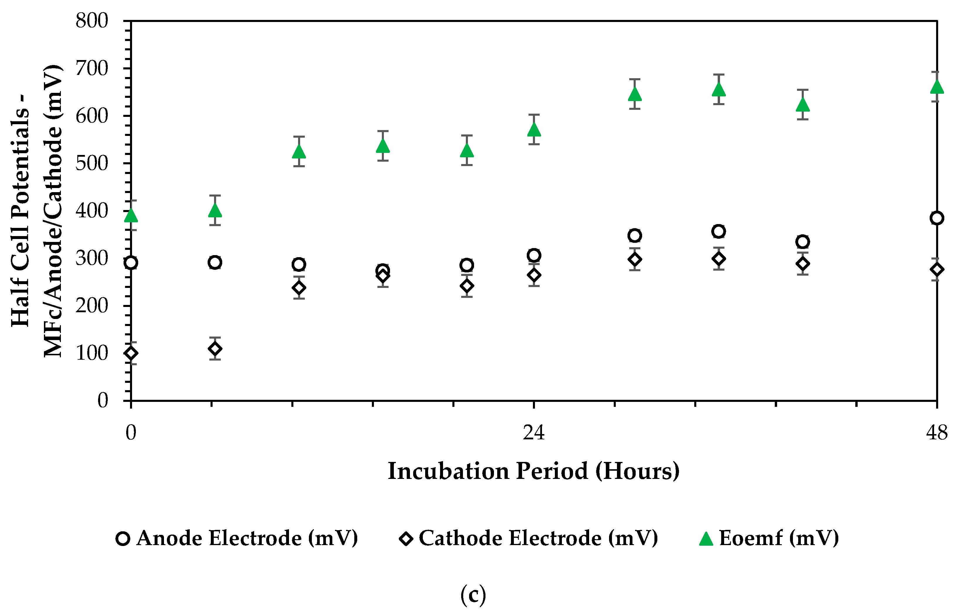
2.6.3. Optimum DCMFC Electromotive Cell Voltage ($E_{cell}^o$) vs. Anodic ($E_{Anode}^o)$ vs. Cathodic ($E_{Cathode}^o)$ Half–Cell Potentials Based on Reference Electrode—AG/AgCl (mV)

In analyzing the electromotive cell voltage ($E_{Cell}^o$) versus the anodic ($E_{Anode}^o$) and cathodic ($E_{Cathode}^o$) half-cell potentials based on a reference electrode (Ag/AgCl, mV), we aimed to understand the electrochemical behavior and chemical energy (cATP) conversion processes within the dual-chamber microbial fuel cell (DCMFC) system. This comparison provides insights into the typical redox reactions that took place at the anode and cathode interfaces, as well as the overall cell voltage generated by these reactions, by examining how the individual half-cell potentials contribute to the overall cell voltage, thereby relating to the efficiency and performance of DCMFCs in converting chemical energy into electrical energy. This analysis instigates to optimize the DCMFC bioelectrochemical capacity more to maximize the overall power output towards enhancing the scalability and applicability of the DCMFC technology in various environmental and energy-related applications. The following plot in Figure 7a–c below closely depicts the attained outcome over the 13 experimental optimization runs. Considering the overall CCV yield production of 700 mV in the combination presented in Figure 7c, it can be derived that high-redox reactions took place at the anode and cathode interfaces, and we can determine the overall cell voltage generated by these reactions. However, Figure 7a also presents a high half-cell overall potential for the entire cell, considering the healthy and highly active anodic bioelectrochemical reactions attested by a partial constant half-cell curve with a high of 445 mV within 10 h of microbial incubation and biodegradation in the DCMFC cell. In this combination, a 10 °C temperature is the critical factor at which it is a clear attribution for the high activity of the Proteobacteria and Bacteriodota, thereby relating to an increased redox bioelectrochemical reaction. Based on these findings, it can be concluded that the redox bioelectrochemical reactions favored both the psychrophilic and mesophilic zone due to the versatility of the active microbes: precisely, the Proteobacteria and Bacteriodota. More insights on its versatility can be found from Shabangu et al. (2024) [46].

2.6.4. Optimum Correlation Curves for Power Density (mW/m²) vs. Current Density (mA/m²) vs. CVV (mV) Yield in Optimizing the DCMFC

In optimizing the dual-chamber microbial fuel cells (DCMFCs), the correlation curves for power density vs. current density vs. closed-circuit voltage yield serve as critical tools for understanding the relationship between these vital performance parameters [56,57] In this study, this optimization process enabled the overall optimization with the RSM–BBD-based scaling-up design and operation of the DCMFC system that delivered enhanced performance and chemical energy conversion capabilities, paving the way for these systems’ experimental validation and hence their recommendation as national grid-connected alternative renewable and sustainable energy generating techniques. Figure 8a–c below shows the attained results during the optimization cycle over 13 experimental observations. These curves depict the relationships among power output (power density), complex substrate active electron flowrate (current density), and overall cell voltage yield in the form of CCV (closed-circuit voltage) under varying conditions, operating the basic operating factors as depicted by the above-detailed RSM–BBD methodology. By analyzing these correlations, it can be identified that finding the optimal balance between current generation and voltage production to maximize the DCMFC’s power output efficiency is crucial and depicts the overall polarization mechanism of the active electrons in this bioelectrochemical system (BES). From a statistical point of view, all three design configurations or ANOVA test combinations yielded highly significant correlations between the three major output electrical variables: CCV (mV), power density (mW/m²), and current density (mA/m²) of R² = 1 precisely. The optimal combination that can possibly exist depicts the overall polarization mechanism of the active electrons for the DCMFC optimization study. As seen in Figure 8a, we attained combination-optimal output variables where the two correlation curves met at 256 mV: 37 mA/m² and 9.6 mW/m² for power density and current density, respectively. As seen in Figure 8b, we attained, at 400 mV, 28 mW/m² and 36 mA/m². Figure 8c presents much higher results than the rest of the design combination factors at 660 mV: 68 mW/vm² and 53 mA/m². Based on the ANOVA test-predicted output values in Figure 5, which presents the numerical optimization ramp plots for optimized output responses in scaling up CCV yield generation in the DCMFC, at 613.71mV, 80.15 mW/m² and 72.38 mA/m² were the predicted responses over 92 iterations and had 77% desirability. Therefore, as seen in Figure 8c, the combination output appeared closest and was strongly considered the reflection of the desired optimum scaling-up operating factors that were highly effective, and statistically and empirically, the model prediction was proven. These findings prove that all three output variables—voltage yield, power density, and current density—are fundamental in finding the optimal operating output, and their correlation can assist in depicting the maximum bioelectrochemical capacity that can be achieved in the DCMFC unit and in any other BES-based technology.

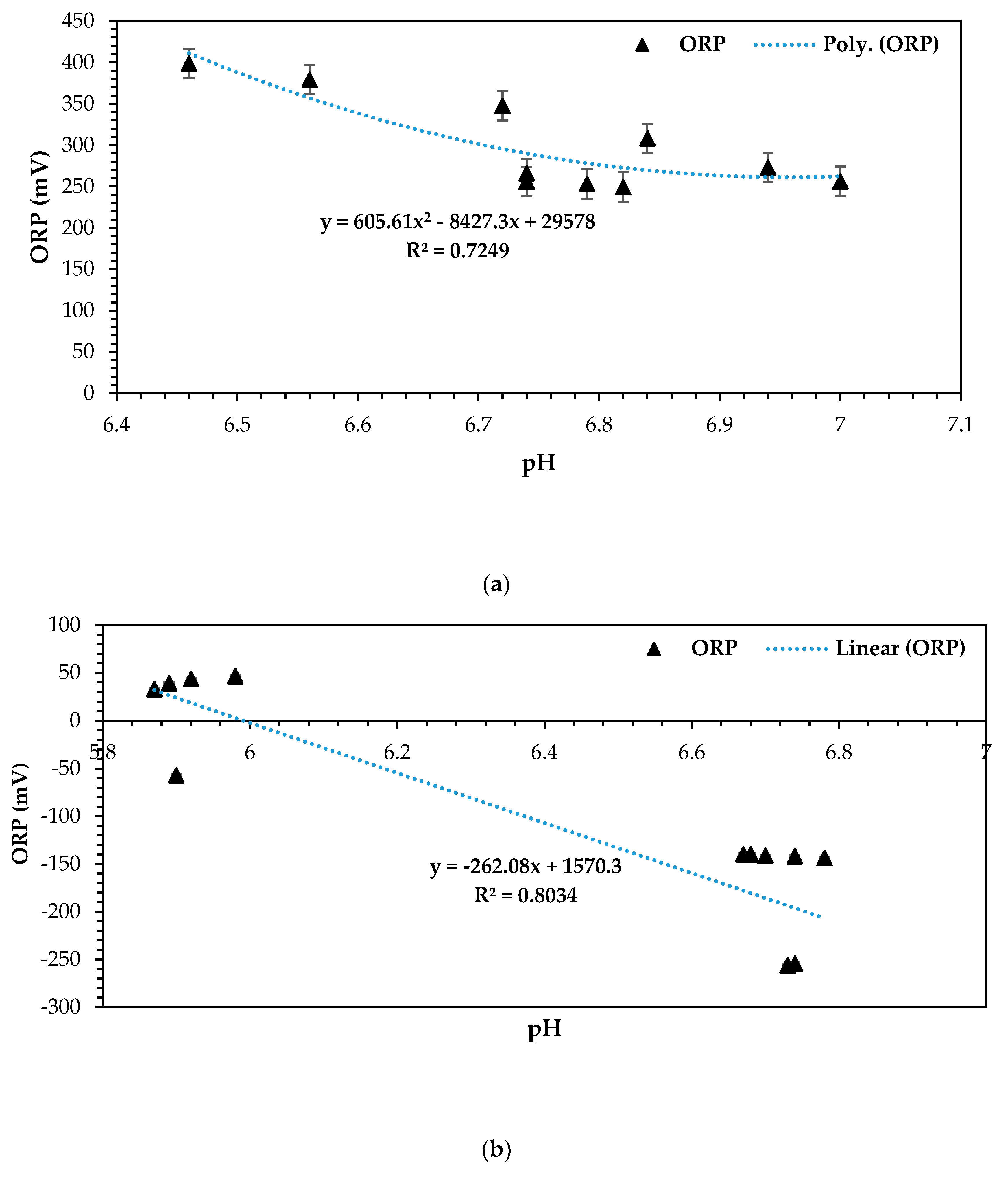
2.6.5. RSM–BBD Application for Optimized ORP (mV) vs. pH Correlation in the DCMFC

In the optimization of microbial fuel cell (MFC) systems, the relationship between the oxidation–reduction potential (ORP) and pH play a crucial role in understanding and enhancing system performance. ORP (mV) intricately indicates the electron transfer potential within the MFC environment [46,56,57,58,59]. pH, on the other hand, measures the acidity or alkalinity of the solution, influencing microbial activity and electrochemical reactions [20,25,58,60,61]. The ORP vs. pH relationship provides insights into the electrochemical and biological processes occurring within the MFC [20,25,58,61]. By analyzing this relationship, one can intricately show the optimal pH conditions that promote microbial activity and electron transfer rates, consequently maximizing DCMFC performance for upscaling, applicability, and practicality in commercial platforms. Additionally, understanding how the ORP changes with pH variations helps in maintaining the stable and efficient operation of the MFC system, which essentially improves the overall electron transference, ultimately promoting the overall CCV generation in this DCMFC unit.

Overall, optimizing the ORP vs. pH relationship in MFC systems will allow for fine-tuning basic operational factors: in this case, a four-factorial, three-level design methodology based on the RSM–BBD empirical optimization approach towards achieving optimal microbial activity, electron transfer kinetics, and, ultimately, improved power generation efficiency in the form of closed-circuit voltage (CCV). The following plots in Figure 9a–c present the relationship between ORP and pH kinetically for all the 13 experimental observations based on the RSM–BBD optimization predictions that were run on different design models as listed in the experimental design output section above. It can be observed that the operating and feasible pH range for these three combinations was between 6 and 8. This pH operating range has been documented previously in numerous studies as favorable for electron transference, the overall flow mechanism, and microbial activity to enhance bioelectricity generation [6,62,63,64,65]. All optimization combinations presented in Figure 9a–c attested to this principle. Moreover, the ORP vs. pH relation was further statistically presented for strong anolyte significance and viability as a perfect electron donor. In principle, a strong oxidation–reduction potential is displayed at negative ORP values, which is clearly shown by Figure 9b,c. Strong correlations of 0.80 and 0.98 were attained, proving the statistical significance of the ORP vs. pH relationship, which is highly conducive for optimized bioelectricity generation [59].

2.6.6. RSM–BBD Application for Optimized Correlation on −ΔGr (J) vs. ORP (mV) Relationship in the DCMFC

In optimizing the generation of bioelectricity in microbial fuel cell (MFC) units, the relationship between Gibbs free energy (ΔG_r) and the oxidation–reduction potential (ORP) is considered vital. ΔG_r represents the energy available from electrochemical reactions occurring within the MFC while ORP indicates the electron transfer potential as intricately stated by previous authors [1,4,9,15,56,58,59]. By analyzing the ΔG_r vs. ORP relationship, the thermodynamic feasibility of electron transfer reactions in the MFC was attained as per the following comparison plots, shown in Figure 10a–c, of Gibbs free energy content (J) vs. the oxidation–reduction potential of the active electrons from the biorefinery-based complex substrates that were seeded as anolytes in the experimental DCMFC optimization observations. Lowering ΔG_r values correspond to more favorable reactions, indicating increased overall cell potential for electricity generation. Similarly, monitoring ORP allows for the adjustment of operational conditions to optimize electron transfer rates and enhance bioelectricity production at very low overall thermodynamic energy electromotive force in the form of Gibbs free energy. Overall, understanding and optimizing the ΔG_r vs. ORP relationship was aimed at designing a typical capable DCMFC unit that would efficiently harness energy from microbial metabolism in the form of cATP, resulting in improved and scaled-up bioelectricity generation in this technology for practical applications at commercial scale. These aspects were further explored in computational modeling for the possibility of grid connection as a reliable alternate energy source, as shown in the following section, and could constitute possible future research work.

Based on Figure 10a above, the optimization findings for the ANOVA test combination at the 1–CCU bi-electrode (surface area) and 10 °C (temperature) and 0.1N (catholyte concentration) resulted in a correlation outcome of (ORP (mV); −ΔGr (J)) and (347.6; −7.23 × 10⁷). These results show that the optimization factor combination at 10 °C and the 1-CCu electrode surface area had almost the least favorability, considering the correlation between ORP and −ΔGr. The positive ORP values depict that more of the overall potential differential capacity was favored from the cathodic chamber from a bioelectrochemical-principal point of view [59]. Moreso, the low temperature of 10 °C may also have seemed to favor the thermodynamic favorability in this design optimization combination, resulting in increased electron and microbial activity in the psychrophilic temperature range, considering the high value of −ΔGr in all the 13 optimization observations. Precisely, the results of the −ΔGr (J) vs. ORP (mV) relationship conclusively and mostly favor the 1-CCU bi–electrode (10 °C and 0.1N), followed (Figure 10c) by the 3-CCU bi-electrode (34 °C and 0.1 N) with (−267.1; −6.39 × 10⁷) and (Figure 10b) the 2-CCU bi-electrode (25 °C and 0.1 N), which resulted in (−254.6; −3.64 × 10⁷). Both combinations shown in Figure 10b, c attained feasibility, and a balance resulted, considering a negative value of ORP, which approved the viability of efficient electron transference and a capable anolyte towards improved thermodynamic favorability. These combinations are closer to the predicted ANOVA test combination of 25 °C, at the 3-CCU bi-electrode, at 48 h and 0.1 N. From a statistical perspective, the third combination in Figure 10c also proved more significant with a correlation factor of R² = 0.79, followed by R² = 0.71 in Figure 10a, then, lastly, Figure 10b at R² = 0.35. The strong correlation between ORP and −ΔGr makes this combination more viable, and this has been proven in by the high and reliable overall design response output variables compared to the rest of the design combinations.

2.7. Summary Results for All Factor Combinations on the Optimization of the DCMFC for Bioelectricity Generation

This section presents Figure 11a–e, a comprehensive summary of the results obtained from the optimization experiments conducted on all operating factor combinations. The motivation for this section lies in the significance of these results in providing a clear understanding of how different combinations of operating factors influence the outcome variables. By analyzing and summarizing the results, we aim to elucidate the impact of each factor and their interactions on the overall performance of the system. Through this summary, one gain insights into the most influential factors and their optimal levels for maximizing the desired responses. This information is crucial for seeking to optimize similar processes or systems as it allows one to identify key variables and fine-tune operating conditions to achieve desired outcomes effectively. Furthermore, by presenting a concise overview of the below results, a deeper understanding of the experimental findings and their implications for further research or practical applications, or rather, the experimental validation and computational scaling up and grid connection simulation, is covered in depth in the following subsections. Overall, this section serves as a valuable resource for interpreting the optimization results and drawing meaningful conclusions to guide future investigations and developments in the field. The following graphical results depict the detailed summarized findings of the optimization runs according to the RSM–BBD methodology over 13 experimental observations.

Based on the findings shown in Figure 11a,c,e, it can be clearly articulated that run no. 13 resulted in the highest CCV yield output, highest power density, highest current density, and highest % CE, which can be attested by the measure of the overall efficiency based on Faraday’s coefficient and the amount of biodegradable COD required to produce current within a given incubation period, proportional to the overall microbial activity, which depends on the nature of the base microbes, which predominantly comprised Proteobacteria and Bacteriodota in for this study, sourced from Logan et al. [9,56,57,66]. Therefore, the ANOVA test predicted the combination of four design factors—catholyte concentration: 0.1 N, HRT: 48 h, electrode surface area: 3-CCu, and temperature: 34 °C. This seemed feasible. This combination can closely match the predicted output based on the ANOVA test’s predicted optimal combination—catholyte concentration: 0.1 N, electrode surface area: 3-CCu, HRT: 48 h, and temperature: 25 °C. The output variables of the predicted combination validation findings are clinically and briefly discussed in the next section. Figure 11b,d present 100% COD and TOC removal and 99% TSS removal, respectively, for runs 5 and 4. These runs were carried out at the following ANOVA test combinations—(i) catholyte concentration: 0.001 N, electrode surface area: 2–CCu, HRT: 96 h, and temperature: 32 °C; (ii) catholyte concentration: 0.001 N, electrode surface area: 3–CCu, HRT: 72 h, and temperature: 30 °C. Both combinations exuded prolonged HRT/incubation periods, which have been scientifically proven to favor the optimal biodegradation of soluble pollutants in the form of COD, BOD, TOC, and TSS. This principle has been observed. From a statistical point of view, run 13 was most feasible and promised optimistic scaling-up output results in the DCMFC using the RSM–BBD predictions. It can be confidently attested that the optimal predicted operating scaling-up factors were adopted and validated as shown in the next section and as deeply discussed by Shabangu et al. [15].

2.8. Validation of Predicted Optimum Voltage Yield and Optimum Complex Substrates Source for Scaling Up Bioelectricity Generation in the DCMFC

This section presents the summary results of validation experiments aimed at comparing the overall voltage capacity of the three distinct substrate sources. The motivation for conducting these experiments lies in the importance of understanding the performance of various substrate sources in bioelectrochemical systems (BESs). The experiments conducted in this section served to address key research questions regarding the efficacy of different substrate sources in generating bioelectricity. By systematically comparing the performance of each substrate, it was identified which substrate source exhibited the highest CCV yields and/or % CE (as shown in Figure 12) and was therefore identified as the most suitable in scaling up the generation of bioelectricity in this DCMFC as the most viable electron donor or anolyte. Through these validation experimental results, valuable insights into the relative performances of different substrate sources and their potential impacts on the overall coulombic efficiency and effectiveness of DCMFC applications were ascertained. Furthermore, the validation experiments ensured the reliability and reproducibility of the findings of this study, thereby strengthening the scientific basis and originality of this research work. The following is a summary of results on three validation runs that were conducted based on the RSM–BBD optimal BBD-predicted scaling-up combination of factors precisely—catholyte dosage: 0.1 N, HRT: 48 h, electrode surface area: 3-CCu (0.01286 m²), and temperature: 25 °C. Figure 12 and

Table 3. Predicted versus experimental results based on the BBD–RSM validation runs, sourced, and reported by Shabangu et al. (2023) [15].

Solution 1 of 92	n	ANOVA Model Predicted Values	Actual Validation Values (Biorefinery-WW)	Actual Validation Values (Mix-WW)	Actual Validation Values (Dairy WW)	Std Dev (Predicted: Actual)
CCV (mV)	3	613.71	640.2	566.9	350.7	-
PD (mW/m2)	3	80.15	61.67	48.36	18.50	-
ID (mA/m2)	3	72.38	49.78	44.08	27.27	-
% COD	3	35.93	62	39	94	39.56
% ${\mathrm{P}\mathrm{O}}_4^{3-}$	3	100.00	61	64	58.1	36.11
% TSS	3	74.20	65	61.4	81	42.65

Std Dev: - means text and logical value False have the value 0.

present the validation-experiment observations for the three distinct wastewater streams as per the optimization sequences. In–depth findings and an analysis of the systems’ performance in terms of the optimization validation output for the DCMFC unit are covered in the validation of RS–BBD scaling-up factors reported by Shabangu et al. [15] in the paper titled “Validation of RSM Predicted Optimum Scaling-Up Factors for Generating Electricity in a DCMFC: MATLAB Design and Simulation Model”. Concisely, the % CE is one of the fundamental thermodynamic favorability-measuring parameters used to assess the overall desirability of a DCMFC unit towards its electron flow mechanism and the rounding up of chemical energy in the conversion in the form of cATP/$∆COD \stackrel{yields}{\to }{G}_{r }^o\left(\frac{J}{s}\right)$, generating, precisely, bioelectricity. Based on the key findings shown in Figure 12, the biorefinery wastewater sourced had an average mean % CE of 2.10% compared to 1.89% and 1.52 for mixed wastewater and dairy wastewater, respectively. These findings validate the concept reported by Shabangu et al. [15,46] in the classification of industrial wastewater sources for the most viable anolyte for increased and scaled-up DCMFC bioelectricity generation.

2.9. Comparison with Previous Studies on RSM–BBD Methodology

This study delved into optimizing DCMFCs using the Box–Behnken design method. It is vital to compare the attained findings of this study with previous studies driven by the goal of improving the overall coulombic efficiency and performance of microbial fuel cells (MFCs) in the form of overall closed-circuit voltage yield through fine–tuned methodical experimentation. By utilizing this design methodology, the target was to identify the best operating conditions for basic scaling-up factors affecting DCMFC electricity production. Furthermore, comparing the attained findings as discussed in the above sections with past research will enhance the understanding on and current progress in MFC current optimization potentials and perhaps identify opportunities for further improvements.

Pandit et al. studied the Box–Behnken design four-factor three-level design methodology in a dual-chamber MFC, considering the following input variables and ranges—cathode surface area: 12–72 cm²; catholyte buffer concentration: 10–100 mM; catholyte pH: 6–8. Pandit et al. [32] had one response variable, power density, and made a key finding: that the surface area of the cathode had significant effect on the power generation. No significant interaction was present among the parameters. Martinez-Conesa et al. [35] reported the findings of the BBD four-factor/three-level design on the effects of temperature (15–35 °C), external resistance (1–100 KΩ), and feed COD concentrations (500–1500 mg COD/L) with anodic pH (5–9). Their operation was conducted in a dual-chamber MFC unit. The key findings were on COD concentration and pH with no significance in terms of overall power density output. Moreover, this study also documented an optimum temperature condition and external resistance of 35 °C and 1 KΩ. Islam et al. [67,68] studied the BBD four-factor/three-level design methodology, noting the effects of an inoculum composition of 30–70%, pH of 6–8, COD concentration of 15,000–45,000 mg COD/L, and HRT of 5–22 days. This study was conducted using a dual-chamber MFC unit. The key findings of this investigation were the interactions between inoculum composition and incubation time, pH, and initial COD assays towards increased MFC performance. Lastly, Zhang et al. [5,8] reported an optimization study on the novel UASB–MFC integrated system for sulfate removal and bioelectricity generation using the RSM–BBD three-factor/three-level design methodology. The operating factors included a pH of 6–8, temperature of 20–40 °C, and oxyfluorfen concentration of 100–200 mg/L. The key finding attained was that the maximum oxyfluorfen degradation capacity of 94.95% was achievable at 31.96 °C, with a pH of 7.65 and oxyfluorfen concentration of 120.05 mg/L.

Precisely, this current study, conducted using the four-factor and three-level Box–Behnken design methodology in a double-chamber MFC unit, was critically optimized considering a full response analysis of eight output variables; the optimum values for CCV yield, % COD removal, current density, power density, % TSS removal, % CE, and % ${\mathrm{P}\mathrm{O}}_4^{3-}$ were 700 mV, 100%, 54.4 mA/m², 73.7 mW/m², 99%, 21.2%, and 100%, respectively. At the optimum conditions, the results revealed a maximum combined desirability of 76.6% out of a total of 92 iterations. The optimal predicted operating combination of a temperature of 25 °C, HRT of 48 h, catholyte concentration of 0.1 M, and electrode surface area of 0.005637–0.01286 m² was instigated with these quantities as actual input variables. Raw industrial wastewater, characterized by a high organic content (with Chemical Oxygen Demand or COD ranging from 250 to 1850 mg/L for biorefinery wastewater and 500 to 3500 mg/L for dairy wastewater, and pH levels between 6 and 7 for both streams), was sourced from a local wastewater treatment plant. This wastewater served as the feedstock for the MFC. The MFC was inoculated with Proteobacteria and Bacteriodota, which acted as electrogenic microorganisms for the bioelectrochemical process. The key findings were positive interactions with the overall closed-circuit voltage, power density, current density, % CE, and the rest of the organic and biodegradation monitoring parameters as presented above. Moreover, the catholyte concentration of 0.1 N was deemed a viable operating electron acceptor or cathodic concentration for optimized bioelectricity generation in this current study. This key finding basically correlates with the above-presented previously conducted studies in terms of most of the basic bioelectrical optimization output concepts in the MFC unit. Furthermore, these outcomes mark a positive shift towards the critical breakthrough for a well-synchronized and balanced and optimized MFC version that will be easily applicable and practically viable at commercial-scale platforms.

3. Materials and Methods

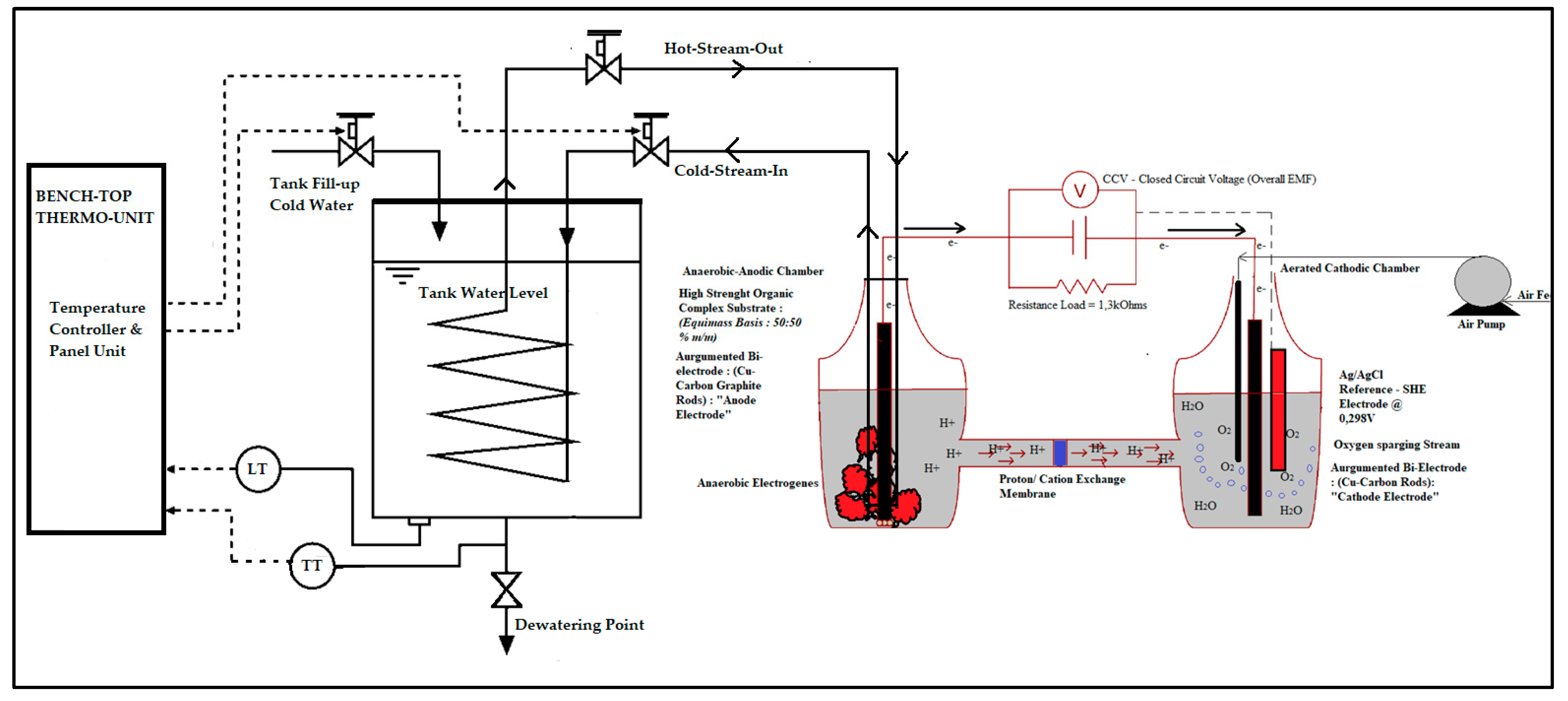
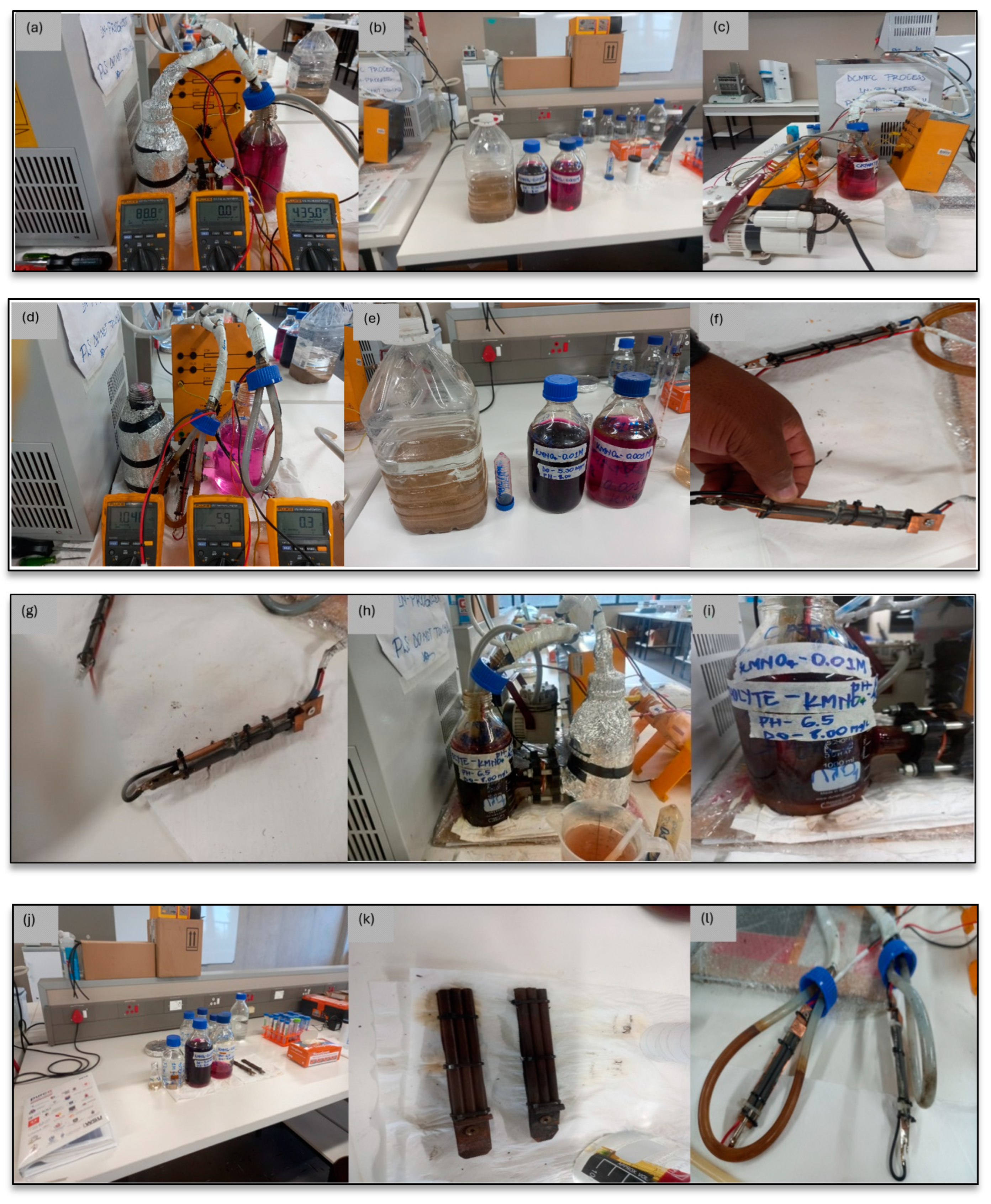
3.1. DCMFC Experimental Configuration and Installation and Commissioning of the DCMFC

The microbial fuel cell (MFC) chamber features a dual-chamber design constructed from two 1-liter Schutt blue cap bottles. These chambers are divided by a Nafion 115^® Proton Exchange Membrane (PEM) from Lyntech, USA, which facilitates the transfer of protons (H+) from the anode chamber to the cathode chamber. The electrodes in the MFC consist of copper bi-electrodes augmented with carbon–graphite electrodes, each occupying a cross-sectional area of 0.005637–0.01286 m². These electrodes are strategically positioned in both the anode and cathode chambers. An external circuit, employing professional-grade positive and negative electrical wires, connects the bi-electrodes, allowing the transfer of electrons generated during the oxidation of organic matter in the anode chamber to the cathode chamber. An external resistance of 1300 Ω is added to the circuit as reported regarding the detailed start-up sequence of the DCMFC in the comparative analysis of organic substrates from industrial wastewater streams for enhanced electricity production using a dual-chamber microbial fuel cell (DCMFC) by Shabangu et al. [46].

The cathode compartment is filled with a standard potassium permanganate solution (${\mathrm{K}\mathrm{M}\mathrm{n}\mathrm{O}}_4^{-})$ with a concentration of 0.1 mol/L, sourced from Logan et al. [28]. As part of novelty of this work, the potassium permanganate concentrate aqueous solution was mixed with raw seawater that had been stored in the incubator at 15 °C after random harvesting from a local ocean beach site in Durban, KwaZulu Natal. This solution was further combined with a controlled and gradual oxygen sparging process, serving as the electron acceptor. Emphasis was made on the strength of the catholyte as it had been proven in previous studies as one of the performance design parameters of the MFC technology towards its scaling-up potentials, etc. Raw industrial wastewater, characterized by high organic content (with Chemical Oxygen Demand or COD ranging from 250 to 1850 mg/L for biorefinery wastewater and 500 to 3500 mg/L for dairy wastewater, and pH levels between 6 and 7 for both streams), was sourced from a local wastewater treatment plant. Biorefinery wastewater was utilized as the major feedstock or raw harvested electron donor and efficient anolyte for the optimization runs in the production of scale-up bioelectricity in the DCMFC unit; this raw wastewater source was already documented as mostly versatile for increased electron donor activity to enhance optimal bioelectricity production by Shabangu et al. [46]. The DCMFC was inoculated with Proteobacteria and Bacteriodota, which acted as electrogenic microorganisms for the bioelectrochemical process. Figure 13 and Figure 14 outline the experimental setup and the precise configuration for operating the DCMFC unit for the optimization that ran using the Response Surface Methodology that adopted the Box–Behnken design approach. This schematic diagram offers a clear depiction of the design features and the layout of the thermo-scientific controller. This is a process block diagram illustrating the distinct components of the dual-chamber microbial fuel cell (DCMFC) and its utilization within the context of the OFAT methodology, specifically examining the effects of psychrophilic and mesophilic temperatures.

Installation and Commissioning of DMFC Cell

On completion of the calibration of the DMM resistor box (De Lorenzo unit—as sourced from Shabangu et al. [46]—start-up sequence for the DCMFC and comparative analysis with detailed DCMFC operating resistance calibration curves), the measurements were taken as shown in Tables S1–S3 in the Supplementary Materials section. For continuity, the test results were deemed acceptable and in accordance with standards for low voltage system. In Table S2, the deviation in each measurement is less than 5%. For the insulation resistance test, the test results were measured and found to be more than 1 MΩ. Polarity was essential for ensuring that the positive was from cathode chamber and negative was from anode chamber. The following Figure 15 is illustrative of the resistance calibration points on the typical bi-electrodes (copper–graphite bi-electrodes) that were utilized in the DCMFC for this study prior to commencing every fed batch and aimed to prepare for each fed batch run and avoid inter-contamination during every experimental run.

3.2. DCMFC Data Analysis

To obtain real-time performance monitoring data for the dual-chamber microbial fuel cell (DCMFC) unit, the following electro-thermodynamic models and expressions were employed, as sourced, and utilized in the start-up sequence for the DCMFC unit used in this study by Shabangu et al. [46]. This involved the measurement of electrical current (I) and voltage (V) at regular 5-h intervals over the course of a precisely controlled 48 h incubation period [28]. Several key parameters, such as Gibbs free energy force, electromotive force (E_Emf), coulombic efficiency (% CE), power densities, and current densities, were also calculated based on the start-up approach and calculation sequence described in comparative analysis of organic substrates conducted by Shabangu et al. [46]. It is important to note that many of these calculation models have been previously documented by other authors and published in reputable scientific journals. The systems’ removal efficiency for the organic performance monitoring parameters was calculated based on Equation (4):

$$\left(\%\right)Removal Efficiency=\frac{C_{initial}-C_{final}}{C_{final}}\times 100\%$$

(4)

Here, (%) removal efficiency is in terms of TOC, COD, TSS, and/or total phosphates (${\mathrm{P}\mathrm{O}}_4^{3-}$); $C_{initial}$ and $C_{final}$ are the initial and final concentrations of the targeted contaminants, respectively.

3.3. Wastewater Sample Analytical Methods

In the performance monitoring phase, wastewater supernatant was subject to analysis both before and after the treatment sequence. The concentration of Chemical Oxygen Demand (COD) was determined using high-range ampoules with a range from 250 to 15,000 mg COD/L. This analysis was carried out with the assistance of a spectrophotometer (HACH, DR3900). TSS, ${\mathrm{P}\mathrm{O}}_4^{3-}$, and TOC levels were measured using a Benchtop DR3200 HACH Spectrophotometer, which was run on triplicates of 3 samples to suffice the replicability analysis and hence provide accurate and reliable parameter measurements. Wastewater fresh samples were harvested from the industrial wastewater treatment plant’s sample points using the grab sampling method. The pHmV, $E_{Cell}^o$, $E_{Anode}^o$, and $E_{Cathode}^o$ half-cell potentials, as well as the full-cell potentials, were also closely monitored by means of the Fluke digital multimeter (DMM) (FLUKE 177—True RMS Digital Multimeter—CAT III 1000 V/CAT IV 600 V). This was accomplished with the aid of a specialized silver–silver reference electrode (Ag/Ag electrode) designed for measuring half-cell potentials in various types of wastewaters under standard operating conditions, particularly within the thermophilic range. The electrode material was PTFE, and it was used in a 3.5 M KCl solution. The electrode specifications included a 4 mm/6 mm design. To ensure data accuracy and reproducibility, all measurements were conducted in replicates, helping eliminate potential human errors during the analytical process.

The temperature control of the MFC during the operational process was efficiently managed with the assistance of a Lab Scientific temperature heater/cooler integrated with a digital temperature controller unit. This setup maintained the temperature within a deviation of less than 3 °C from the set point value. Additionally, during the operation of the semi-batch processes, online monitoring of all the above-mentioned operating parameters was performed using a Hanna Multiparameter device equipped with a universal data logger probe. This allowed for the simultaneous measurement and recording of various crucial operating parameters. Table S4 underneath presents the detailed pollutant contaminants contained in the three sources of wastewater.

3.4. Design of Experiment (DoE) Using Response Surface Methodology (RSM)

The Box–Behnken design in Design Expert version 11 was used to ascertain the number of experimental runs to be assayed for the optimization of four independent variables, i.e., temperature (X₁), electrode surface area (X₂), catholyte concentration (X₃), and hydraulic residence time (X₄), on the generation of voltage yield—closed circuit voltage (Y₁), power density (Y₂), current density (Y₃), coulombic efficiency (CE%) (Y₄), Chemical Oxygen Demand (COD) (Y₅), total phosphates (${\mathrm{P}\mathrm{O}}_4^{3-}$) (Y₆), total suspended solids (TSS) (Y₇), and total organic carbon (TOC) (Y₈). The codes, ranges, and levels of the independent variables in RSM design are shown in

Table 4. Codes, ranges, and levels of independent variables of Box–Behnken design in RSM.

Factor	Name	Units	Type	Minimum	Maximum	Coded Low	Coded High	Mean	Std. Dev.
A	Catholyte	mg/L	Numeric	0	0,1	−1 ↔ 0.00	+1 ↔ 0.10	0.0257	0.0425
B	HRT	Hours	Numeric	48	96	−1 ↔ 48.00	+1 ↔ 96.00	66.46	17.4
C	Temperature	°C	Numeric	10	40	−1 ↔ 10.00	+1 ↔ 40.00	26.46	9.13
D	Surface area	m2	Numeric	1	3	−1 ↔ 1.00	+1 ↔ 3.00	2.08	0.8623

.

The quadratic empirical model for predicting the response i.e., $Y$, is derived as a function of the levels of the independent variables expressed according to Equations (5) and (6):

$$Y={\beta }_0+\sum _{i=1}^k{\beta }_i{x}_i+\sum _{i=1}^k{\beta }_{ii}{x}_i^2+\sum _{i=1}^{k=1}\sum _{j=i+1}^k{\beta }_{ij}{x}_i{x}_j+\epsilon$$

(5)

$$x_i=\frac{z_i-z_0}{{∆z}_i}$$

(6)

Here, $x_i$ and $x_j$ are coded independent variables; $i$ denotes the linear coefficient, $j$ is the quadratic coefficient, $\beta$ is the coefficient of regression, and $k$ denotes the number of factors studied and optimized by the experiment; $\epsilon$ denotes the random error; $z_i$ and $z_0$ are the code and uncoded values of the $i\mathrm{t}\mathrm{h}$ independent variable, respectively; and ${∆z}_i$ is the step change value between the low level (−1) and high level (+1). According to Nair et al. [26], in RSM, codification of variables is performed to normalize the variables. It is imperative to note that independent variables may have units and orders of magnitude, and the codification ensures that all independent variables affect the specified responses evenly. The Box–Behnken design methodology in RSM is optimized in two phases: the numerical method, then, subsequently, the graphical method. The sequence of optimization and iterative predictive steps are carried out in this section of the statistical software, aimed towards setting up the best possible predictive factors to attain an optimized desired response on the MFC unit. The basic factors considered for scaling-up possibilities are tabulated in

Table 5. BBD layout on the MFC optimization.

Response Name	Units	Observations	Minimum	Maximum	Mean	Std. Dev.	Ratio	Model
CCV	mV	13	40.2	700	190.48	18.88	17.41	Reduced Quadratic
PD	mW/m2	13	0.13	73.74	9,99	20.36	544.68	2FI
ID	mA/m2	13	2.70	54.43	18.47	15	20.11	2FI
COD	%	13	18	92	42.54	17.7	5.11	Reduced Quadratic
${\mathbf{P}\mathbf{O}}_4^{3-}$	%	13	28.1	68	47.32	11.8	2.42	Reduced Quadratic
CE	%	13	0.079	21.59	3.59	6.29	273	Linear
TSS	%	13	32.9	98.8	60.59	18.02	3	Reduced Quadratic
TOC	%	13	18.9	100	45.92	26.25	5.29	Reduced 2FI

, which presents a sequence of predictive numerical values towards optimum operating combination of factors. Figure 16 is a typical flowchart that outlines the steps involved in the Box–Behnken design methodology, starting from defining independent variables and ending with achieving the desired response on the MFC unit. Each step represents a crucial stage in the experimental optimization process that was instigated in the optimization of the dual-chamber microbial fuel cell operation for scaling up the production of bioelectricity.

4. Conclusions

To examine curvature in the response, quadratic response surface modeling was utilized. The Box–Behnken design (BBD) was employed as an independent quadratic response surface design, devoid of an embedded factorial or fractional design. This design necessitates three levels of each factor and yields fewer experimental runs compared to the central composite design with an equivalent number of factors. The focus of this study was on the application of RSM on the use of MFCs for bioelectricity production whilst treating purely industrial wastewater using the Box–Behnken design optimization method. The end results of CCV yield, % COD removed, and maximum current density achieved, optimum power density achieved, optimum coulombic efficiency % CE, % TSS removal, % TOC removal and % total phosphate ${(\mathrm{P}\mathrm{O}}_4^{3-})$ removal indicated that based on the Analysis of Variance (ANOVA) test and Fit Statistics, the reduced quadratic model, reduced two-factor interaction (2FI) and linear model attained sound and practicable results instead of the single application of the suggested linear model only, a combined approach for each response was adopted as presented in Table 5. This is also due to the nature of the BBD methodology tailored for the quadratic response surface modeling design. The ANOVA test results subsequently demonstrated considerable high p-value, predicted R², and adjusted R² values. The CCV yield model attained a significantly high R² of 0.99, together with the other electrical monitoring parameters, power density and current density. This aspect proved the feasibility of the optimization test by ANOVA test. Second-order regression models were also generated using design expert software to predict CCV yield, % COD removed, current density, power density, faraday/coulombic efficiency (% CE), % TSS removal, % TOC removal, % ${(\mathrm{P}\mathrm{O}}_4^{3-})$ removal, at the combinations of temperature, HRT, surface area and catholyte dosage. The models were validated by predicted versus actual plots, residuals versus runs, and leverage versus run number graphs. The outcome of the results revealed that the optimal MFC conditions were surface area (m²) of three carbon copper rods (3-CCu-bi-electrode), temperature of 25 $℃$, and catholyte dosage of potassium permanganate of 0.1 mg/L. Under these optimum operating conditions, the RSM revealed the highest voltage yield of 700 mV, % COD removal of 100, and current density, power density, % TSS removal, % CE, and % ${\mathrm{P}\mathrm{O}}_4^{3-}$ were 54.4 mA/m², 73.7 mW/m², 99%, 21.2%, and 100%, respectively. The results revealed a desirability performance of 76.6% for overall voltage yield generation. Therefore, based on the findings of this optimization study, conclusively it can be articulated that the performance of DCMFCs for optimized bioelectricity generation whilst treating raw industrial wastewater substrates correlates with the catholyte concentration dosage at the optimum temperature and optimum bi-electrode surface area ANOVA test design combination. Based on the above empirical models, this study recommends the DCMFC as a practical and applicable technology for sustainable battery power source suitable for consideration as part of the national grid connection in retrospect to the current South African energy crisis. In-depth findings and system performance analysis of the optimization validation output for the DCMFC unit are discussed in the study by Shabangu et al. [15], titled “Validation of RSM Predicted Optimum Scaling-Up Factors for Generating Electricity in a DCMFC: MATLAB Design and Simulation Model.” Furthermore, future experimental analysis proving the long-term operational performance of the DCMFC battery as a reliable and sustainable bioelectricity energy source is strongly recommended based on the findings of this optimization study. The attained percentage coulombic efficiency (% CE) serves as a fundamental parameter to evaluate the overall desirability of the DCMFC unit in terms of electron flow mechanisms and the conversion of chemical energy into bioelectricity. According to the results presented in Figure 12, biorefinery wastewater exhibited an average % CE of 2.10% while mixed wastewater and dairy wastewater recorded values of 1.89% and 1.52%, respectively. These findings support the notion that biorefinery wastewater may serve as the most viable anolyte for enhancing and scaling up DCMFC bioelectricity generation, as reported by Shabangu et al. [15,46].

References

1. Raychaudhuri, A.; Behera, M. Review of the Process Optimization in Microbial Fuel Cell using Design of Experiment Methodology. J. Hazard. Toxic Radioact. Waste 2020, 24, 4020013. [Google Scholar] [CrossRef]
2. Kloch, M.; Toczyłowska-Mamí, R. Toward Optimization of Wood Industry Wastewater Treatment in Microbial Fuel Cells-Mixed Wastewaters Approach. Available online: https://www.mdpi.com/journal/energies (accessed on 22 May 2024).
3. Hyun, K.; Kim, S.; Kwon, Y. Performance evaluations of yeast based microbial fuel cells improved by the optimization of dead zone inside carbon felt electrode. Korean J. Chem. Eng. 2021, 38, 2347–2352. [Google Scholar] [CrossRef]
4. Ahn, Y.; Hatzell, M.C.; Zhang, F.; Logan, B.E. Different electrode configurations to optimize performance of multi-electrode microbial fuel cells for generating power or treating domestic wastewater. J. Power Sources 2014, 249, 440–445. [Google Scholar] [CrossRef]
5. Zhang, B.; Zhang, J.; Yang, Q.; Feng, C.; Zhu, Y.; Ye, Z.; Ni, J. Investigation, and optimization of the novel UASB–MFC integrated system for sulfate removal and bioelectricity generation using the response surface methodology (RSM). Bioresour. Technol. 2012, 124, 1–7. [Google Scholar] [CrossRef]
6. Gil, G.C.; Chang, I.S.; Kim, B.H.; Kim, M.; Jang, J.K.; Park, H.S.; Kim, H.J. Operational parameters affecting the performance of a mediator-less microbial fuel cell. Biosens Bioelectron. 2003, 18, 327–334. [Google Scholar] [CrossRef] [PubMed]
7. Identifying Optimized Conditions for Concurrent Electricity Production and Phosphorus Recovery in a Mediator-Less Dual Chamber Microbial Fuel Cell—ScienceDirect. Available online: https://www.sciencedirect.com/science/article/abs/pii/S0306261918312789?fr=RR-2&ref=pdf_download&rr=84264e8bfbe54ecc (accessed on 8 January 2024).
8. Xia, C.; Zhang, D.; Pedrycz, W.; Zhu, Y.; Guo, Y. Models for Microbial Fuel Cells: A critical review. J. Power Sources 2018, 373, 119–131. [Google Scholar] [CrossRef]
9. Logan, B.E.; Hamelers, B.; Rozendal, R.; Schröder, U.; Keller, J.; Freguia, S.; Aelterman, P.; Verstraete, W.; Rabaey, K. Microbial fuel cells: Methodology and technology. Environ. Sci. Technol. 2006, 40, 5181–5192. [Google Scholar] [CrossRef]
10. Guelpa, E.; Verda, V. Model for optimal malfunction management in extended district heating networks. Appl. Energy 2018, 230, 519–530. [Google Scholar] [CrossRef]
11. Cano, V.; Chrispim, M.C.; de Souza, T.S.O.; Penteado, E.D. Novel bioelectrochemical processes focused on nitrogen in wastewater: Energy generation and resource recovery. Water Manag. Circ. Econ. 2023, 233–272. [Google Scholar]
12. Wang, L.; Tai, Y.; Zhao, X.; He, Q.; Hu, Z.; Li, M. Phosphorus recovery directly from sewage sludge as vivianite and simultaneous electricity production in a dual chamber microbial fuel cell. J. Environ. Chem. Eng. 2023, 11, 110152. [Google Scholar] [CrossRef]
13. Hosseinpour, M.; Vossoughi, M.; Alemzadeh, I. An efficient approach to cathode operational parameters optimization for mi-crobial fuel cell using response surface methodology. J. Environ. Health Sci. Eng. 2014, 12, 33. [Google Scholar] [CrossRef]
14. Benayyad, A.; Kameche, M.; Kebaili, H.; Innocent, C. Design of a Microbial Fuel Cell Used as a Biosensor of Pollution Emitted by Oxidized Organic Matter. In Advances in Renewable Hydrogen and Other Sustainable Energy Carriers; Springer Nature: Singapore, 2021; pp. 279–284. [Google Scholar]
15. Shabangu, K.P.; Mthembu, N.; Chetty, M.; Bakare, B.F. Validation of RSM Predicted Optimum Scaling-Up Factors for Generating Electricity in a DCMFC: MATLAB Design and Simulation Model. Fermentation 2023, 9, 856. [Google Scholar] [CrossRef]
16. Noori, T.; Ganta, A.; Tiwari, B.R. Recent Advances in the Design and Architecture of Bioelectrochemical Systems to Treat Wastewater and to Produce Choice-Based Byproducts. J. Hazard. Toxic Radioact. Waste 2020, 24, 04020023. [Google Scholar] [CrossRef]
17. Muchtar, A.; Tambunan, A.H.; Machfud, M. Preliminary Analysis of Single-Flash Geothermal Power Plant by Using Exergy Method: A Case Study from Ulubelu Geothermal Power Plant in Indonesia Bioethanol from Brown Seaweed View Project PRODUCTION SYSTEM DESIGN OF BANANA BASED ENERGY BAR INDUSTRY View Project. 2018. Available online: https://www.researchgate.net/publication/335175433 (accessed on 22 May 2024).
18. Aghababaie, M.; Farhadian, M.; Jeihanipour, A.; Biria, D. Environmental Technology Reviews Effective Factors on the Performance of Microbial Fuel Cells in Wastewater Treatment—A Review. 2015. Available online: https://www.tandfonline.com/action/journalInformation?journalCode=tetr20 (accessed on 8 January 2024).
19. Sun, D.; Gao, Y.; Hou, D.; Zuo, K.; Chen, X.; Liang, P.; Zhang, X.; Ren, Z.J.; Huang, X. Energy-neutral sustainable nutrient recovery incorporated with the wastewater purification process in an enlarged microbial nutrient recovery cell. J. Power Sources 2018, 384, 160–164. [Google Scholar] [CrossRef]
20. He, Z.; Huang, Y.; Manohar, A.K.; Mansfeld, F. Effect of electrolyte pH on the rate of the anodic and cathodic reactions in an air-cathode microbial fuel cell. Bioelectrochemistry 2008, 74, 78–82. [Google Scholar] [CrossRef] [PubMed]
21. Zhang, X.; He, W.; Ren, L.; Stager, J.; Evans, P.J.; Logan, B.E. COD removal characteristics in air-cathode microbial fuel cells. Bioresour. Technol. 2015, 176, 23–31. [Google Scholar] [CrossRef] [PubMed]
22. Cercado-Quezada, B.; Delia, M.-L.; Bergel, A. Testing various food-industry wastes for electricity production in microbial fuel cells. Bioresour. Technol. 2010, 101, 2748–2754. [Google Scholar] [CrossRef]
23. Kim, J.H.; An, B.M.; Lim, D.H.; Park, J.Y. Electricity production and phosphorous recovery as struvite from synthetic wastewater using magnesium-air fuel cell electrocoagulation. Water Res. 2018, 132, 200–210. [Google Scholar] [CrossRef]
24. Blöcher, C.; Niewersch, C.; Melin, T. Phosphorus recovery from sewage sludge with a hybrid process of low-pressure wet oxidation and nanofiltration. Water Res. 2012, 46, 2009–2019. [Google Scholar] [CrossRef]
25. Zhang, L.; Li, C.; Ding, L.; Xu, K.; Ren, H. Influences of initial pH on performance and anodic microbes of fed-batch microbial fuel cells. J. Chem. Technol. Biotechnol. 2011, 86, 1226–1232. [Google Scholar] [CrossRef]
26. Zhao, H.; Kong, C.-H. Elimination of pyraclostrobin by simultaneous microbial degradation coupled with the Fenton process in microbial fuel cells and the microbial community. Bioresour. Technol. 2018, 258, 227–233. [Google Scholar] [CrossRef] [PubMed]
27. Peng, L.; Dai, H.; Wu, Y.; Peng, Y.; Lu, X. A comprehensive review of phosphorus recovery from wastewater by crystallization processes. Chemosphere 2018, 197, 768–781. [Google Scholar] [CrossRef] [PubMed]
28. Pasupuleti, S.B.; Srikanth, S.; Mohan, S.V.; Pant, D. Continuous mode operation of microbial fuel cell (MFC) stack with dual gas diffusion cathode design for the treatment of dark fermentation effluent. Int. J. Hydrog. Energy 2015, 40, 12424–12435. [Google Scholar] [CrossRef]
29. Elhenawy, S.; Khraisheh, M.; AlMomani, F.; Al-Ghouti, M.; Hassan, M.K. From Waste to Watts: Updates on Key Applications of Microbial Fuel Cells in Wastewater Treatment and Energy Production. Sustainability 2022, 14, 955. [Google Scholar] [CrossRef]
30. Mohammadi, A.; Khadir, A.; Tehrani, R.M.A. Optimization of nitrogen removal from an anaerobic digester effluent by electro-coagulation process. J. Environ. Chem. Eng. 2019, 7, 103195. [Google Scholar] [CrossRef]
31. Numbi, B.; Xia, X. Systems optimization model for energy management of a parallel HPGR crushing process. Appl. Energy 2015, 149, 133–147. [Google Scholar] [CrossRef]
32. Pandit, S.; Ghosh, S.; Ghangrekar, M.M.; Das, D. Performance oof an Anion Exchange Membrane in Association with Cathodic Parameters in a Dual Chamber Microbial Fuel Cell. 2012. Available online: www.sciencedirect.com (accessed on 8 January 2024).
33. Puig, S.; Serra, M.; Coma, M.; Balaguer, M.D.; Colprim, J. Simultaneous domestic wastewater treatment and renewable energy production using microbial fuel cells (MFCs). Water Sci. Technol. 2011, 64, 904–909. [Google Scholar] [CrossRef]
34. Jadhav, D.A.; Carmona-Martínez, A.A.; Chendake, A.D.; Pandit, S.; Pant, D. Modeling, and optimization strategies towards perfor-mance enhancement of microbial fuel cells. Bioresour. Technol. 2021, 320, 124256. [Google Scholar] [CrossRef] [PubMed]
35. Martínez-Conesa, E.J.; Ortiz-Martínez, V.M.; Salar-García, M.J.; Ríos, A.P.D.L.; Hernández-Fernández, F.J.; Lozano, L.J.; Godínez, C. A Box–Behnken Design-Based Model for Predicting Power Performance in Microbial Fuel Cells Using Wastewater. Chem. Eng. Commun. 2016, 204, 97–104. [Google Scholar] [CrossRef]
36. Behera, M.; Ghangrekar, M.M. Optimization of Operating Conditions for Maximizing Power Generation and Organic Matter Removal in Microbial Fuel Cell. J. Environ. Eng. 2017, 143, 04016090. [Google Scholar] [CrossRef]
37. Capodaglio, A.G.; Cecconet, D.; Molognoni, D. An integrated mathematical model of microbial fuel cell processes: Bioelectro-chemical and microbiologic aspects. Processes 2017, 5, 73. [Google Scholar] [CrossRef]
38. Chen, S.; Patil, S.A.; Brown, R.K.; Schröder, U. Strategies for optimizing the power output of microbial fuel cells: Transitioning from fundamental studies to practical implementation. Appl. Energy 2018, 233–234, 15–28. [Google Scholar] [CrossRef]
39. Recio-Garrido, D.; Perrier, M.; Tartakovsky, B. Modeling, optimization, and control of bioelectrochemical systems. Chem. Eng. J. 2016, 289, 180–190. [Google Scholar] [CrossRef]
40. Kadivarian, M.; Karamzadeh, M. Electrochemical modeling of microbial fuel cells performance at different operating and structural conditions. Bioprocess Biosyst. Eng. 2019, 43, 393–401. [Google Scholar] [CrossRef] [PubMed]
41. Gupta, R.; Sethi, S.; Bharshankh, A.; Sahu, R.; Biswas, R. A perspective on Bio-Electrochemical System (BES) as a tool for boosting the performance of the nonperforming anaerobic units. Clean. Circ. Bioeconomy 2023, 6, 100066. [Google Scholar] [CrossRef]
42. Optimization of Enhanced Bioelectrical Reactor with Electricity from Microbial Fuel Cells for Groundwater Nitrate Removal [Internet]. Available online: https://www.tandfonline.com/doi/epdf/10.1080/09593330.2015.1096962?needAccess=true (accessed on 8 January 2024).
43. Bagchi, S.; Behera, M. Pharmaceutical wastewater treatment in ceramic separator MFC: Optimisation of operating parameters to improve organic removal and power generation. Clean. Circ. Bioeconomy 2023, 6, 100063. [Google Scholar] [CrossRef]
44. Shabangu, K.P.; Bakare, B.F.; Bwapwa, J.K. Microbial Fuel Cells for Electrical Energy: Outlook on Scaling-up and Application Possibilities Towards South African Energy Grid. Sustainability 2022, 14, 14268. [Google Scholar] [CrossRef]
45. Armah, E.K.; Chetty, M.; Adedeji, J.A.; Kukwa, D.T.; Mutsvene, B.; Shabangu, K.P.; Bakare, B.F. Emerging Trends in Wastewater Treatment Technologies: The Current Perspective. In Promising Techniques for Wastewater Treatment and Water Quality Assessment; IntechOpen: London, UK, 2021. [Google Scholar]
46. Shabangu, K.P.; Mthembu, N.; Chetty, M.; Bwapwa, J.K.; Bakare, B.F. A comparative analysis of organic substrates from industrial wastewater streams for enhanced electricity production using a double chamber microbial fuel cell (DCMFC). Energy Rep. 2024, 11, 3050–3063. [Google Scholar] [CrossRef]
47. He, L.; Huang, G.H.; Lu, H.W. A stochastic optimization model under modeling uncertainty and parameter certainty for groundwater remediation design-Part I. Model development. J. Hazard. Mater. 2010, 176, 521–526. [Google Scholar] [CrossRef] [PubMed]
48. Rahmani Eliato, T.; Pazuki, G.; Majidian, N. Potassium permanganate as an electron receiver in a microbial fuel cell Potassium permanganate as an electron receiver in a microbial fuel cell. Energy Sources Part A Recovery Util. Environ. Eff. 2016, 38, 644–651. [Google Scholar]
49. Tahir, C.A.; Pásztory, Z.; Agarwal, C.; Csóka, L. Electricity Generation and Wastewater Treatment with Membrane-Less Microbial Fuel Cell. Appl. Microbes Environ. Microb. Biotechnol. 2022, 235–261. [Google Scholar]
50. ATP Monitoring Technology for Microbial Growth Control in Potable Water Systems. Available online: https://www.spiedigitallibrary.org/conference-proceedings-of-spie/6203/62030N/ATP-monitoring-technology-for-microbial-growth-control-in-potable-water/10.1117/12.673425 (accessed on 12 February 2024).
51. García, V.G.; Bartolomé, M.M. Rural electrification systems based on renewable energy: The social dimensions of an innovative technology. Technol. Soc. 2010, 32, 303–311. [Google Scholar] [CrossRef]
52. Marone, A.; Varrone, C.; Fiocchetti, F.; Giussani, B.; Izzo, G.; Mentuccia, L.; Rosa, S.; Signorini, A. Optimization of substrate composition for biohy-drogen production from buffalo slurry co-fermented with cheese whey and crude glycerol, using microbial mixed culture. Int. J. Hydrog. Energy 2015, 40, 209–218. [Google Scholar] [CrossRef]
53. Jadhav, D.A.; Ghangrekar, M.M. Optimising the proportion of pure and mixed culture in inoculum to enhance the performance of microbial fuel cells. Int. J. Environ. Technol. Manag. 2020, 23, 50. [Google Scholar] [CrossRef]
54. Fang, F.; Zang, G.-L.; Sun, M.; Yu, H.-Q. Optimizing multi-variables of microbial fuel cells for electricity generation with an integrated modeling and experimental approach. Appl. Energy 2013, 110, 98–103. [Google Scholar] [CrossRef]
55. Ishii, S.; Suzuki, S.; Norden-Krichmar, T.M.; Wu, A.; Yamanaka, Y.; Nealson, K.H.; Bretschger, O. Identifying the microbial communities and operational conditions for optimized wastewater treatment in microbial fuel cells. Water Res. 2013, 47, 7120–7130. [Google Scholar] [CrossRef] [PubMed]
56. Logan, B.E.; Rabaey, K. Conversion of Wastes into Bioelectricity and Chemicals by Using Microbial Electrochemical Technologies. Science 2012, 337, 686–690. [Google Scholar] [CrossRef] [PubMed]
57. Logan, B.E.; Regan, J.M. Electricity-producing bacterial communities in microbial fuel cells. Trends Microbiol. 2006, 14, 512–518. [Google Scholar] [CrossRef] [PubMed]
58. Yu, R.-F.; Chen, H.-W.; Cheng, W.-P.; Lin, Y.-J.; Huang, C.-L. Monitoring of ORP, pH and DO in heterogeneous Fenton oxidation using nZVI as a catalyst for the treatment of azo-dye textile wastewater. J. Taiwan Inst. Chem. Eng. 2014, 45, 947–954. [Google Scholar] [CrossRef]
59. Khumalo, S.M.; Bakare, B.F.; Rathilal, S.; Tetteh, E.K. Characterization of South African Brewery Wastewater: Oxidation-Reduction Potential Variation. Water 2022, 14, 1604. [Google Scholar] [CrossRef]
60. Silva-Illanes, F.; Tapia-Venegas, E.; Schiappacasse, M.C.; Trably, E.; Ruiz-Filippi, G. Impact of hydraulic retention time (HRT) and pH on dark fermentative hydrogen production from glycerol. Energy 2017, 141, 358–367. [Google Scholar] [CrossRef]
61. Margaria, V.; Tommasi, T.; Pentassuglia, S.; Agostino, V.; Sacco, A.; Armato, C.; Chiodoni, A.; Schilirò, T.; Quaglio, M. Effects of pH variations on anodic marine con-sortia in a dual chamber microbial fuel cell. Int. J. Hydrog. Energy 2017, 42, 1820–1829. [Google Scholar] [CrossRef]
62. Kim, M.Y.; Kim, C.; Ainala, S.K.; Bae, H.; Jeon, B.-H.; Park, S.; Kim, J.R. Metabolic shift of Klebsiella pneumoniae L17 by electrode-based electron transfer using glycerol in a microbial fuel cell. Bioelectrochemistry 2018, 125, 1–7. [Google Scholar] [CrossRef] [PubMed]
63. Yu, J.; Park, Y.; Widyaningsih, E.; Kim, S.; Kim, Y.; Lee, T. Microbial fuel cells: Devices for real wastewater treatment, rather than electricity production. Sci. Total. Environ. 2021, 775, 145904. [Google Scholar] [CrossRef]
64. Kim, J.R.; Min, B.; Logan, B.E. Evaluation of procedures to acclimate a microbial fuel cell for electricity production. Appl. Microbiol. Biotechnol. 2005, 68, 23–30. [Google Scholar] [CrossRef] [PubMed]
65. Kim, B.H.; Chang, I.S.; Gadd, G.M. Challenges in microbial fuel cell development and operation. Appl. Microbiol. Biotechnol. 2007, 76, 485–494. [Google Scholar] [CrossRef]
66. Ahn, Y.; Logan, B.E. Effectiveness of domestic wastewater treatment using microbial fuel cells at ambient and mesophilic tem-peratures. Bioresour. Technol. 2010, 101, 469–475. [Google Scholar] [CrossRef] [PubMed]
67. Ahmed, S.F.; Mofijur, M.; Islam, N.; Parisa, T.A.; Rafa, N.; Bokhari, A.; Klemeš, J.J.; Mahlia, T.M.I. Insights into the development of microbial fuel cells for generating biohydrogen, bioelectricity, and treating wastewater. Energy 2022, 254, 124163. [Google Scholar] [CrossRef]
68. Khandaker, S.; Das, S.; Hossain, M.T.; Islam, A.; Miah, M.R.; Awual, M.R. Sustainable approach for wastewater treatment using mi-crobial fuel cells and green energy generation—A comprehensive review. J. Mol. Liq. 2021, 344, 117795. [Google Scholar] [CrossRef]
Figure 1. Effect of scaling-up factors and responses on CCV yield: (a) CCV vs. catholyte dose (b) CCV vs. HRT (c) CCV vs. temperature; and (d) CCV vs. surface area.
Energies 17 02740 g001aEnergies 17 02740 g001b
Figure 2. Predicted vs. actual graphs for (a) CCV yield, (b) power density (mW/m2), (c) current density (mA/m2), (d) % COD, (e) % P O 4 3 , (f) % CE, (g) % TSS, and (h) % TOC.
Energies 17 02740 g002aEnergies 17 02740 g002b
Figure 3. Leverage vs. runs for (a) CCV yield, (b) power density (mW/m2), (c) current density (mA/m2), (d) % COD, (e) % P O 4 3 , (f) % CE, (g) % TSS, and (h) % TOC.
Energies 17 02740 g003aEnergies 17 02740 g003b
Figure 4. Residual vs. experimental runs: (a) CCV yield, (b) power density (mW/m2), (c) current density (mA/m2), (d) % COD, (e) % P O 4 3 , (f) % CE, (g) % TSS, and (h) % TOC.
Energies 17 02740 g004aEnergies 17 02740 g004b
Figure 5. Numerical optimization ramp plots: solutions for the optimized output responses for scaling up CCV yield generation in the DCMFC.
Energies 17 02740 g005
Figure 6. CCV vs. OCV plots at 3 optimum operating combinations: (a) 1–CCu–bi–electrode (surface area) at 10 °C and 0.1 N (catholyte dosage), (b) 2-CCu-bi-electrode (surface area) at 25 °C and 0.1 N (catholyte dosage), and (c) 3–CCu–bi–electrode (surface area) at 34 °C and 0.1 N (catholyte dosage) (optimum CCV–OCV plot based on predicted RSM–BBD factors).
Energies 17 02740 g006aEnergies 17 02740 g006b
Figure 7. Half-cell potential plots ( E c e l l o vs. E A n o d e o vs. E C a t h o d e o ): (a) 1-CCu-bi-electrode (surface area) at 10 °C and 0.1 N (catholyte dosage), (b) 2-CCu-bi-electrode (surface area) at 25 °C and 0.1 N (catholyte dosage), and (c) 3-CCu-bi-electrode (surface area) at 34 °C and 0.1 N (catholyte dosage).
Energies 17 02740 g007aEnergies 17 02740 g007b
Figure 8. Correlation of CVV (mV) vs. power density (mW/m2) vs. current density (mA/m2). (a) Correlation curve at 1–CCU–bi–electrode (surface area) and 10 °C and 0.1 N (catholyte dosage). (b) Correlation curve at 2–CCU–bi–electrode and 25 °C and 0.1 N (catholyte dosage). (c) Correlation curve at 3–CCU bi-electrode and 34 °C and 0.1 N (catholyte dosage).
Energies 17 02740 g008aEnergies 17 02740 g008b
Figure 9. (a) ORP (mV) vs. pH at 1–CCU bi-electrode (surface area) and 10 °C and 0.1 N (catholyte dosage), (b) ORP (mV) vs. pH at 2–CCU bi-electrode and 25 °C and 0.1 N (catholyte dosage), and (c) ORP (mV) vs. pH at 3–CCU bi-electrode and 34 °C and 0.1 N (catholyte dosage).
Energies 17 02740 g009aEnergies 17 02740 g009b
Figure 10. −ΔGr (J) vs. ORP (mV) for 3 distinct combinations: (a) −ΔGr (J) vs. ORP (mV) at 1–CCU bi–electrode (surface area) and 10 °C and 0.1 N (catholyte dosage), (b) −ΔGr (J) vs. ORP (mV) at 2–CCU bi–electrode and 25 °C and 0.1 N (catholyte dosage), and (c) −ΔGr (J) vs. ORP (mV) at 3–CCU bi–electrode and 34 °C and 0.1 N (catholyte dosage).
Energies 17 02740 g010
Figure 11. (a) CCV yield vs. power density vs. current density for all DoE optimizations, (b) power density vs. % COD response output for all DoE optimizations, (c) CCV yield vs. % COD response output for all DoE optimizations, (d) power density vs. TOC response output or all DoE optimizations, and (e) % COD vs. % TSS vs. % CE output responses for all DoE optimizations.
Energies 17 02740 g011aEnergies 17 02740 g011b
Figure 12. % CE comparison plot for wastewater sources for scaling up bioelectricity generation in a DCMFC, sourced from Shabangu et al. [15].
Energies 17 02740 g012
Figure 13. Benchtop DCMFC for generating bioelectricity treating raw industrial wastewater source, mixed wastewater, with Scientific Thermo Control connected to the benchtop fabricated 1 L dual-chamber microbial fuel cell (DCMFC), sourced from Shabangu et al. [46].
Energies 17 02740 g013
Figure 14. DCMFC components for optimization and scaling-up four-factor layout: (a) catholyte setpoint of 0.001 N; (b) different catholytes prepared with seawater combination with variable potassium permanganate concentrations; (c) catholyte at 0.01 N; (d) catholyte at 0.001 N and 1-CCu electrode configuration; (e) combined catholyte, either with 0.001 or 0.1 N KMnO4; (f) and (g) 1-CCu-electrode (surface area); (h) 0.1 N and 3-CCu-bioelectrode (surface area and catholyte); (i) 0.01 N catholyte concentration; (j) catholyte options: seawater, industrial buffer (pH control), and design catholyte—KMnO4—0.1 and 0.001 N; (k) 3-CCu-bi-electrode (surface area); (l) 2-CCu-bi-electrode (surface area); (m) full scaling-up operation at 0.1 N and 3-CCu-bi-electrode and 34 °C; (n) operation at 10 °C; and (o) catholyte concentration–KMnO4–0.1 N, with 1-3 CCu bi-electrode displayed and complete temperature manifold configuration, sourced from the start operation reported by Shabangu et al. [46].
Energies 17 02740 g014aEnergies 17 02740 g014b
Figure 15. The resistance calibration points on the bi–electrodes of the DCMFC unit. (1) Cathode copper–graphite bi–electrode mounted with 1 graphite rod (1–CCu–bi–electrode). (2) Negative terminal port across the fluke multimeters. (3) Positive terminal port across the fluke multimeters. (4) Anode made of copper–graphite bi–electrode (1–CCu–1–bi–electrode).
Energies 17 02740 g015
Figure 16. Box–Behnken design layout in Response Surface Methodology.
Energies 17 02740 g016