
Thermal Resistance Modeling for the Optimal Design of EE and E/PLT Core-Based Planar Magnetics

Abstract
:1. Introduction
2. Thermal Resistance for the Design of Planar Magnetics
2.1. Planar EE and E/PLT Cores
- The external area: Aext. Its value is computed by summing all the external surfaces of the core and the windings;
- The effective volume: Ve. This value defines a hypothetical ring core having the same magnetic properties as the planar core [15].
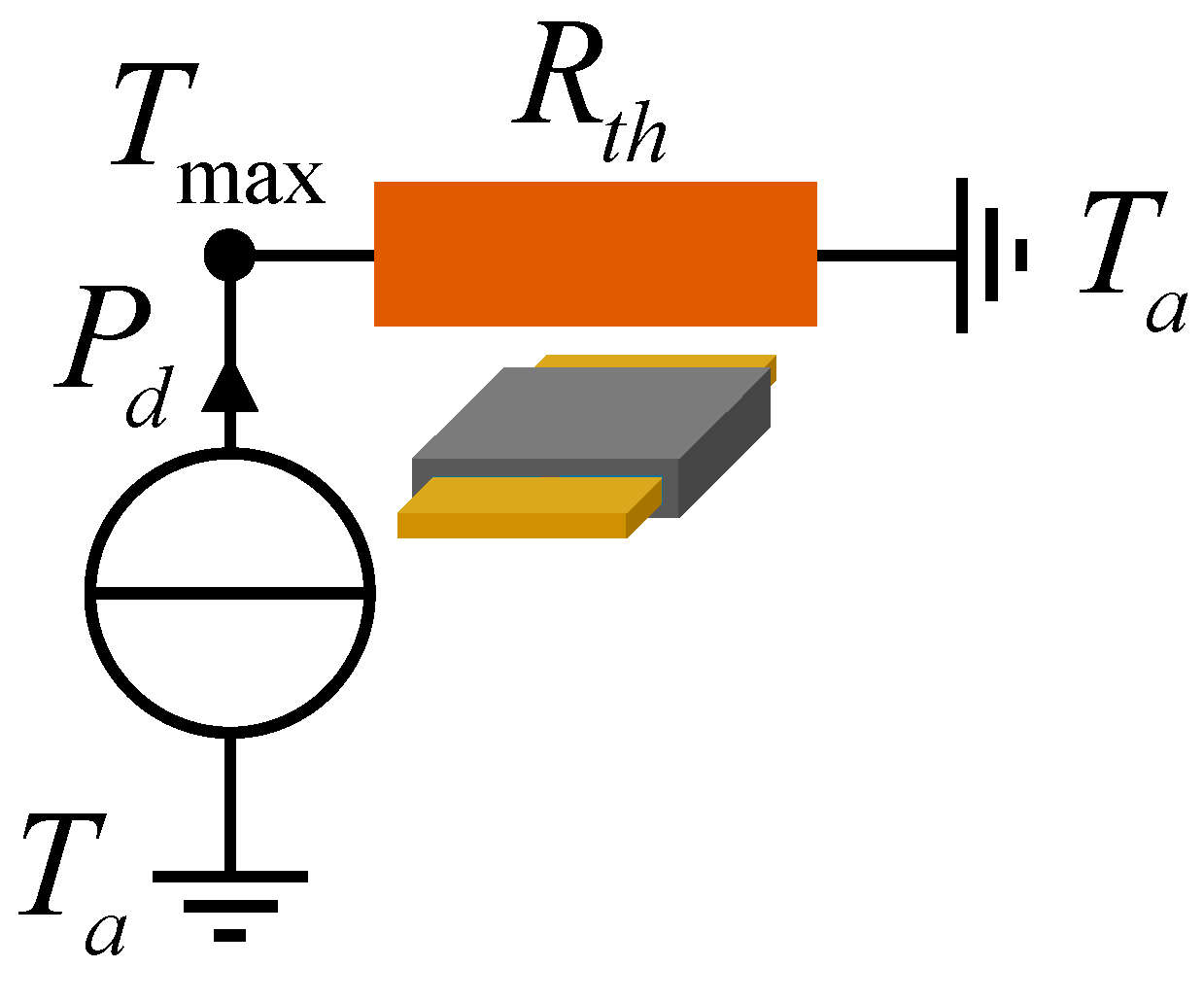
2.2. Can a Single Global Thermal Resistance Be Used for Planar Magnetics?
- Total losses inside the transformer (13 W) are divided into two parts: 6.5 W for the winding and 6.5 W for the core;
- Thermal connection between the winding and the core is perfect;
- Ambient temperature is set to 25 °C;
- A heat exchange coefficient of 14 W·K−1·m−2 is applied to all the external areas of the transformer [20].
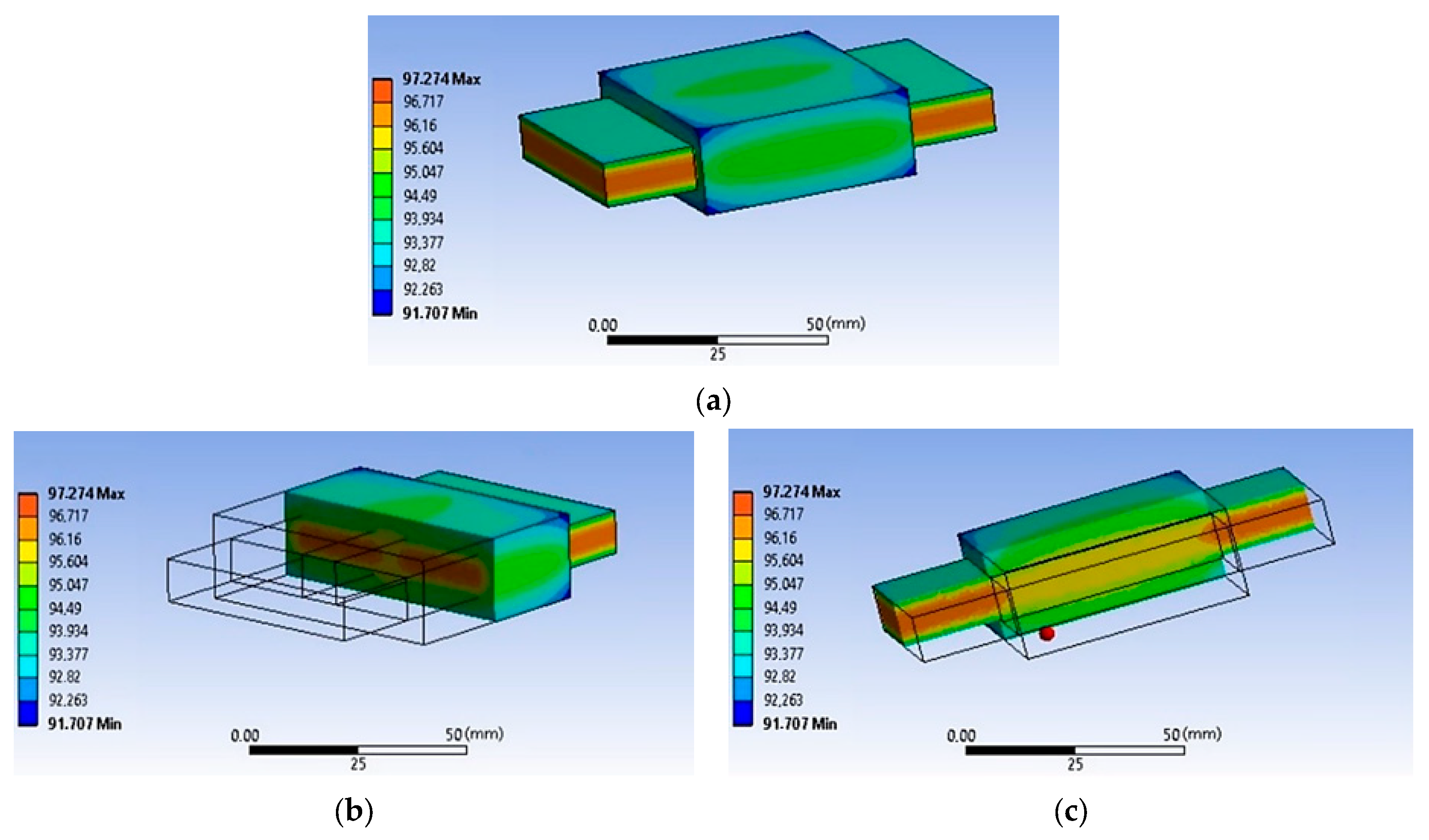
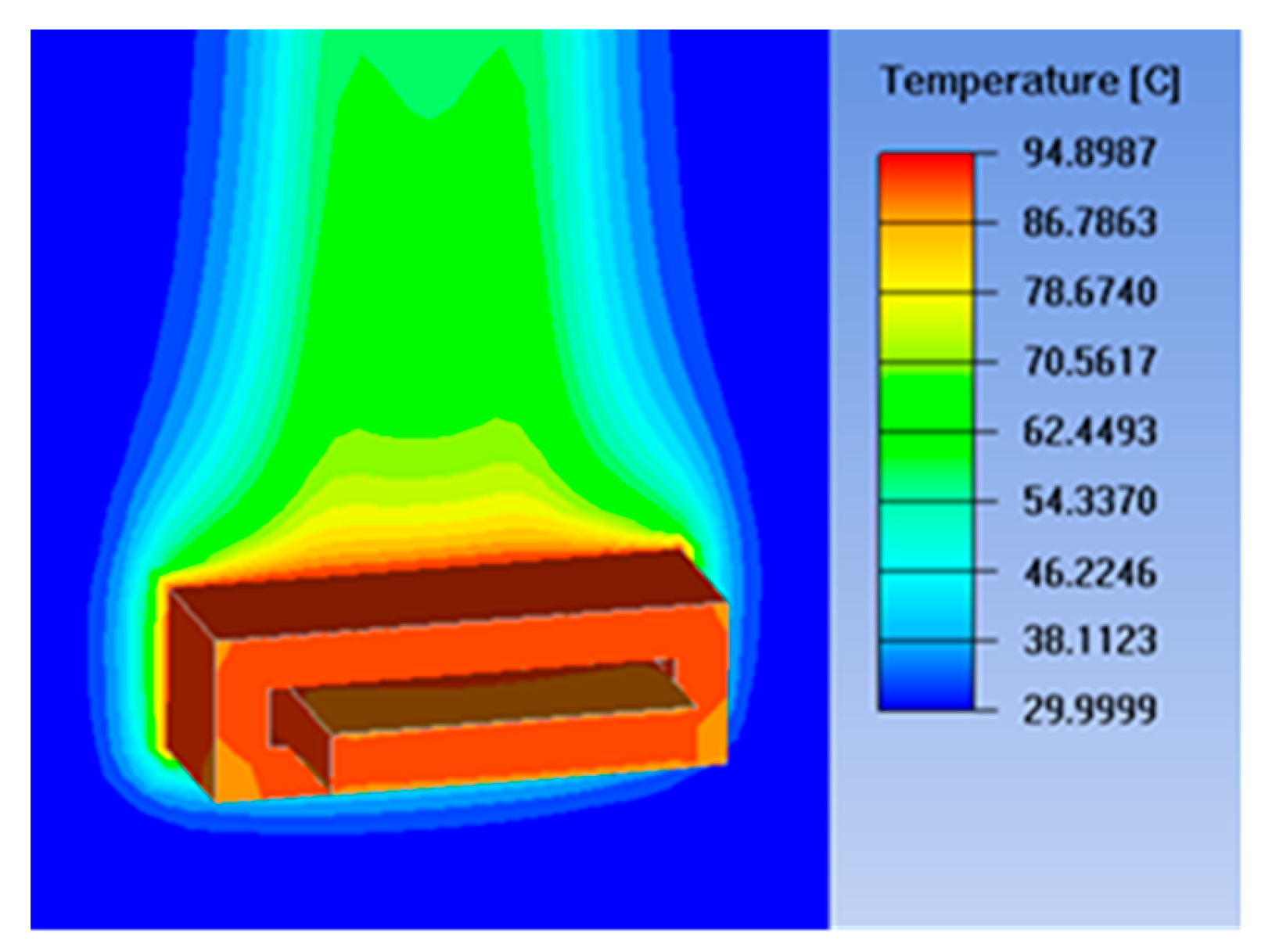
2.3. Impact of Parameters on the Planar Component Temperature Distribution
- Case 4, where the total losses are localized in the core;
- Case 5, where the losses are split between the core and the winding;
- Case 6, where the losses are localized only in the winding.
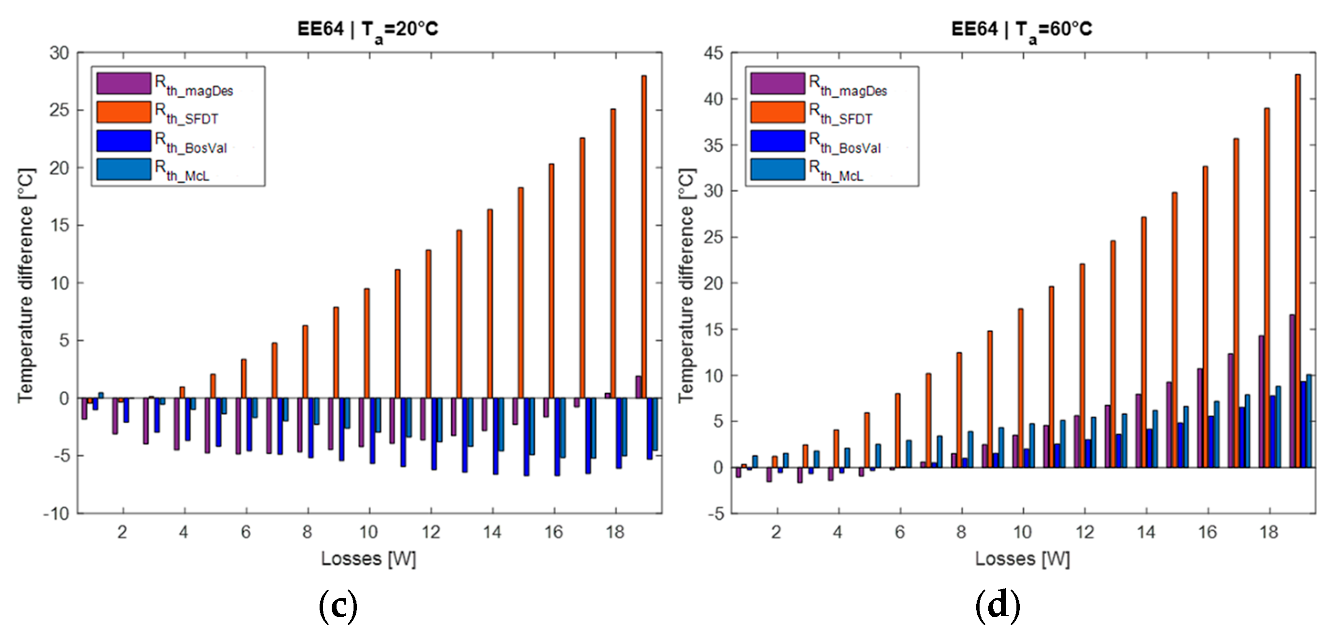
2.4. Comparison of Planar Magnetic Core Thermal Resistance Modeling
3. Study of Thermal Resistance Variation According to Power Losses and Ambient Temperature
3.1. Study Methodology
- The total losses (Pd) that vary from 1 W to Pmax (Table 5) by step of 1 W;
- The ambient temperature (Tamb) that takes discrete values: 20 °C, 30 °C, 40 °C, 50 °C and 60 °C.
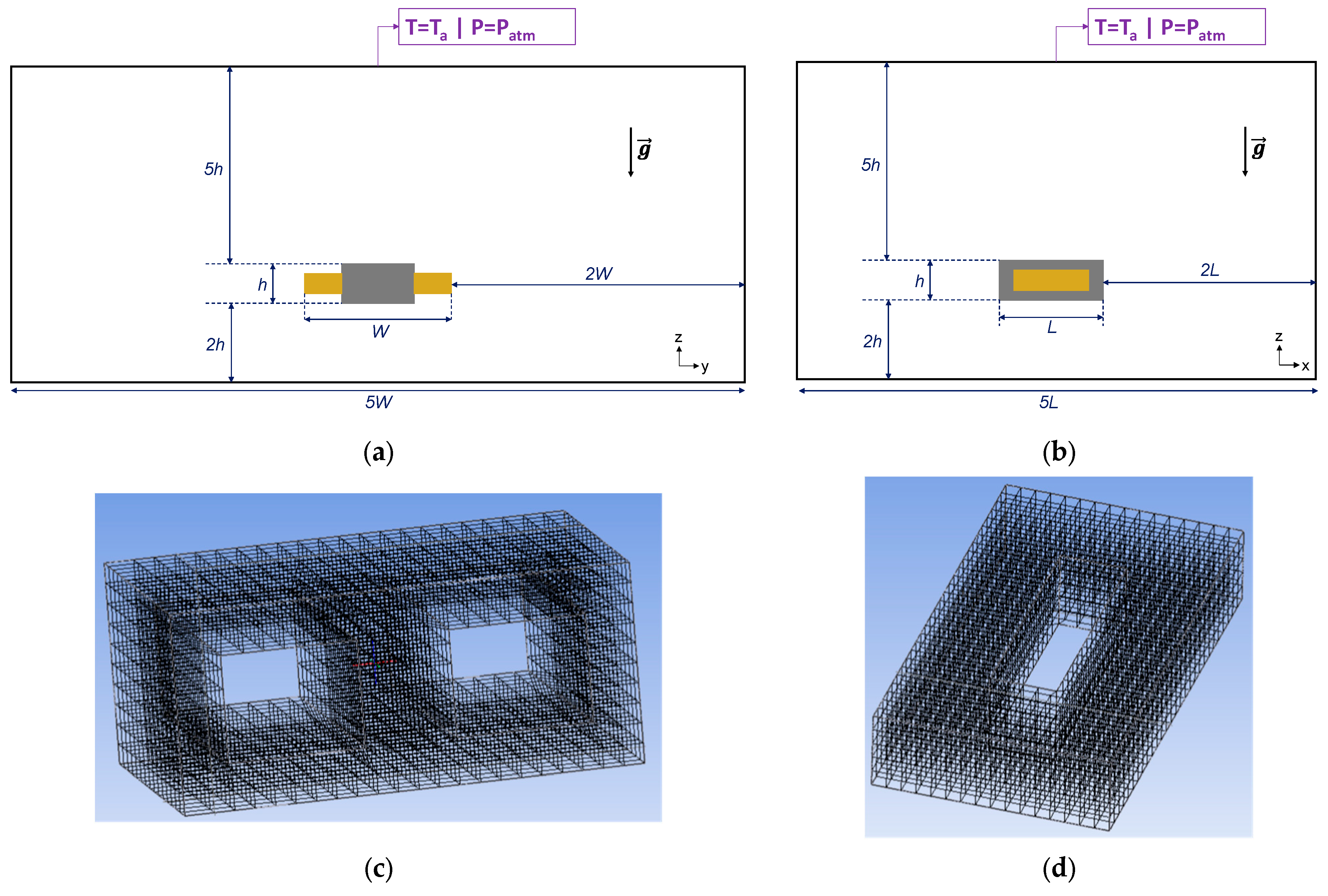
3.2. CFD Simulation Parameters
- Temperature of the external area of the domain is fixed to Ta.
- Air pressure is set to atmospheric pressure:
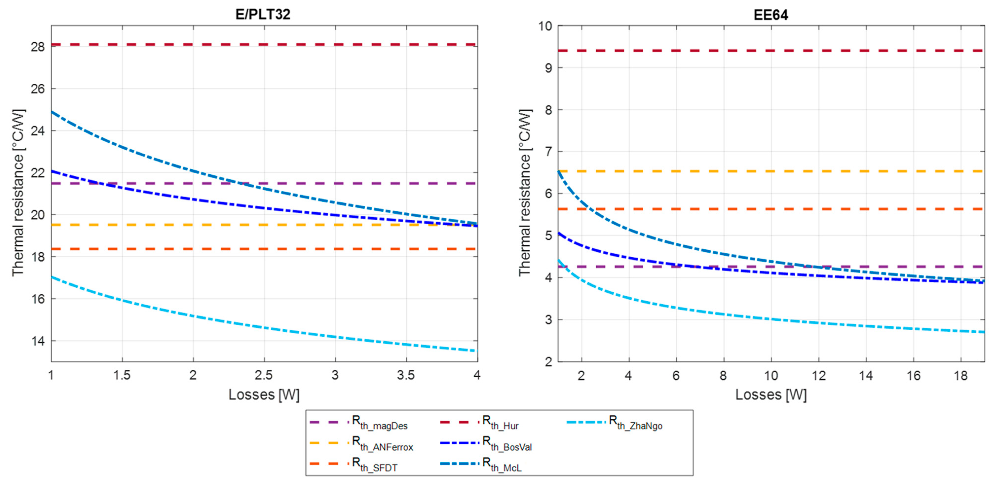
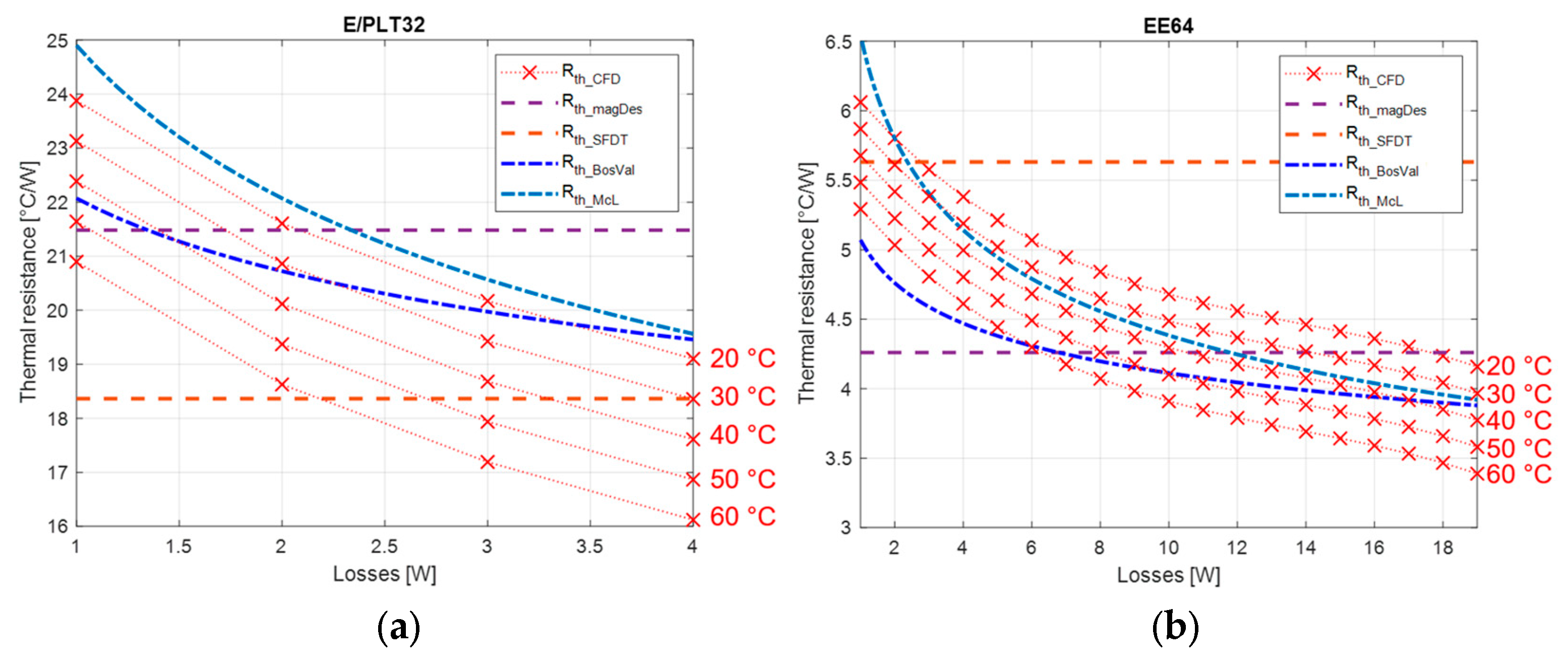
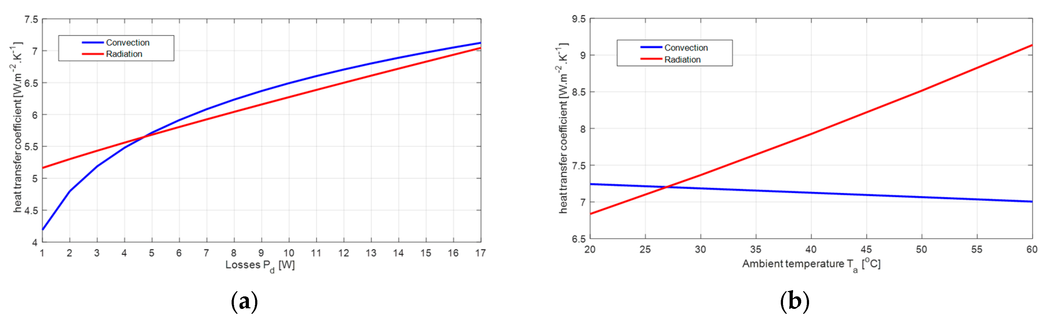
3.3. Results and Analysis
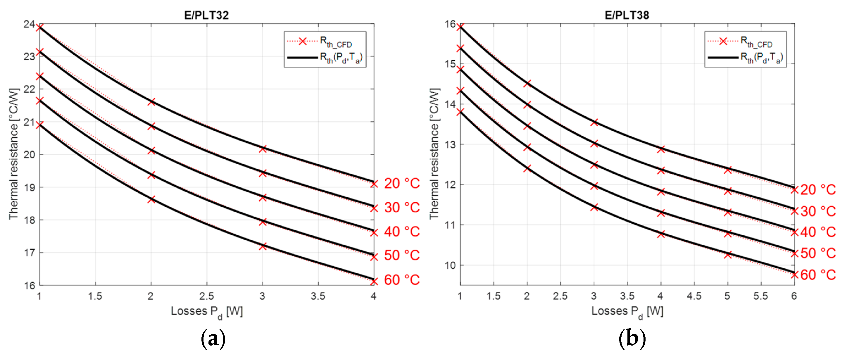
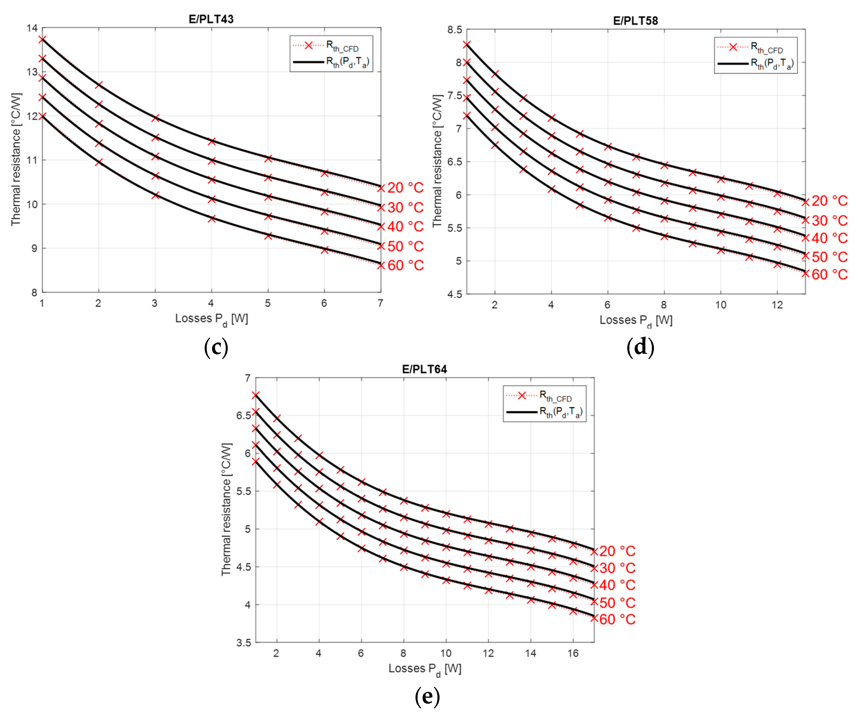
4. Analytical Modeling of Thermal Resistance Variation
- Power range: (Table 5);
- Ambient temperature:
5. Validation and Discussion
5.1. Comparison with CFD Simulation Results
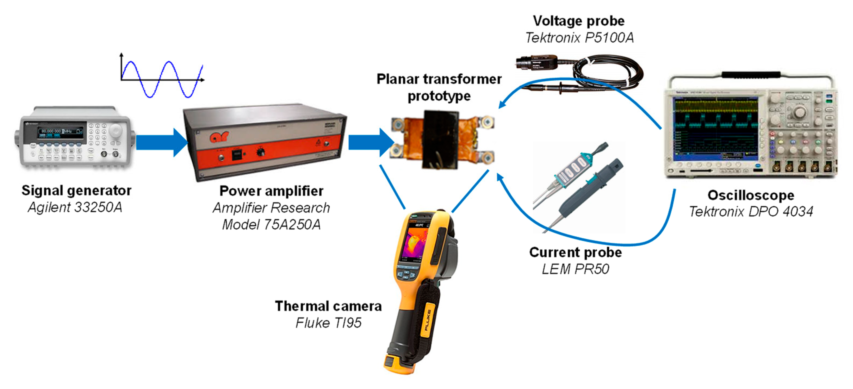
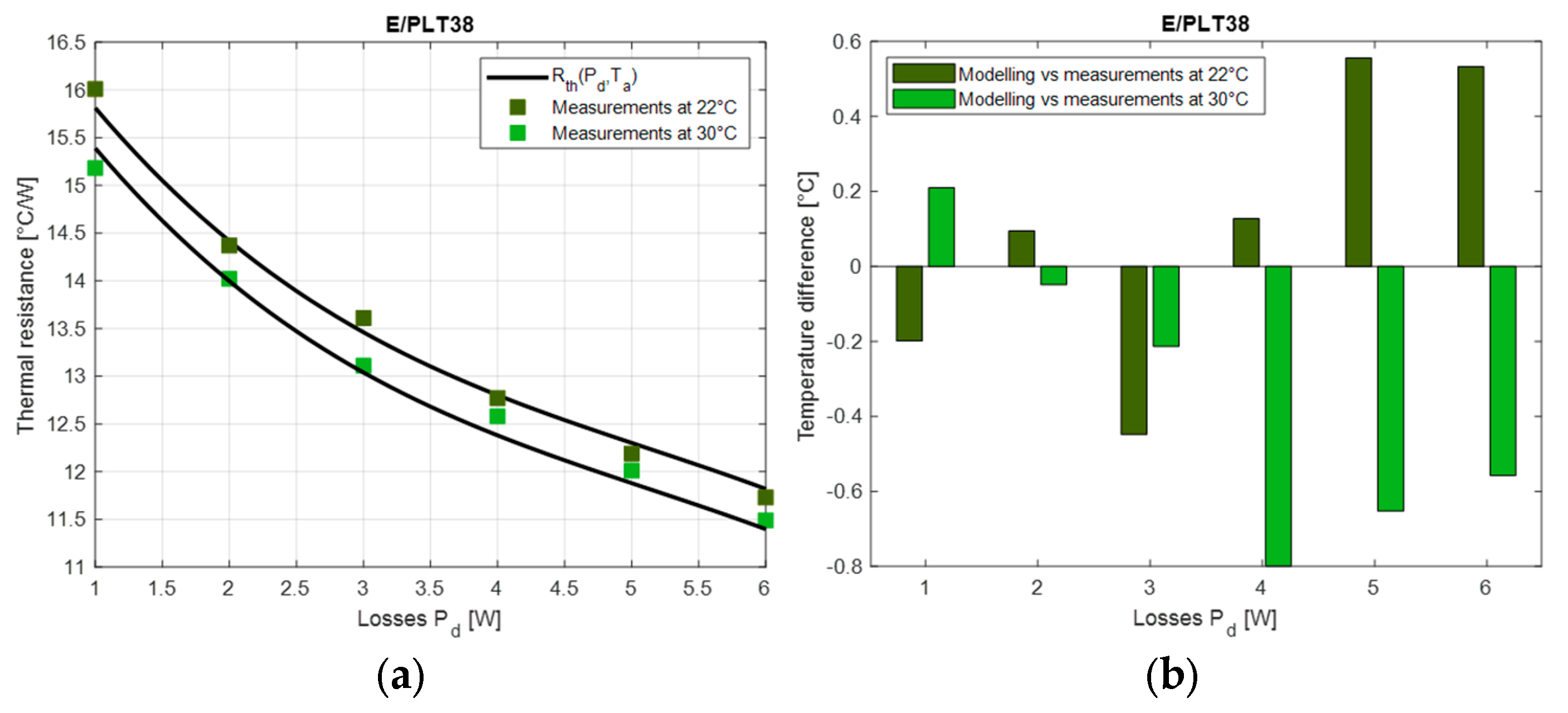
5.2. Experimental Validation
5.3. Discussion
6. Conclusions
Author Contributions
Funding
Data Availability Statement
Conflicts of Interest
References
- Guan, Y.; Wang, Y.; Xu, D.; Wang, W. A 1 MHz Half-Bridge Resonant DC/DC Converter Based on GaN FETs and Planar Magnetics. IEEE Trans. Power Electron. 2017, 32, 2876–2891. [Google Scholar] [CrossRef]
- Zhang, Z.; Ngo, K.D.T. Multi-megahertz quasi-square-wave flyback converter using eGaN FETs. IET Power Electron. 2017, 10, 1138–1146. [Google Scholar] [CrossRef]
- Ouyang, Z.; Andersen, M.A.E. Overview of Planar Magnetic Technology—Fundamental Properties. IEEE Trans. Power Electron. 2014, 29, 4888–4900. [Google Scholar] [CrossRef]
- Ngoua Teu Magambo, J.S.; Bakri, R.; Margueron, X.; Le Moigne, P.; Mahe, A.; Guguen, S.; Bensalah, T. Planar Magnetic Components in More Electric Aircraft: Review of Technology and Key Parameters for DC–DC Power Electronic Converter. IEEE Trans. Transp. Electrif. 2017, 3, 831–842. [Google Scholar] [CrossRef]
- Planar Transformers for EV On-Board Chargers & DC-DC Converter Applications. Available online: https://standexelectronics.com/planar-magnetics/planar-transformers-for-ev-on-board-chargers-dc-dc-converter-applications/ (accessed on 25 April 2024).
- Son, W.-J.; Lee, B.K. Design of Planar Transformers for LLC Converters in High Power Density On-Board Chargers for Electric Vehicles. Energies 2023, 16, 6757. [Google Scholar] [CrossRef]
- Lee, D.-W.; Lim, J.-H.; Lee, D.-I.; Youn, H.-S. A High-Power-Density Active-Clamp Converter with Integrated Planar Transformer. Energies 2022, 15, 5609. [Google Scholar] [CrossRef]
- Magnetics Designer—Personal Computer Circuit Design Tools. Available online: http://www.intusoft.com/lit/Magdes.pdf (accessed on 25 April 2024).
- Muldoon, W.J. Analytical design optimization of electronic power transformers. In Proceedings of the Power Electronics Specialists Conference, Syracuse, NY, USA, 13–15 June 1978; pp. 216–225. [Google Scholar]
- Design of Planar Power Transformers. Available online: http://ferroxcube.home.pl/appl/info/plandesi.pdf (accessed on 25 April 2024).
- Ferroxcube Soft Ferrites Design Tool (SFDT). Available online: https://www.ferroxcube.com/en-global/design_tool/index (accessed on 25 April 2024).
- Hurley, W.G.; Wölfle, W.H. Transformers and Inductors for Power Electronics—Theory, Design and Applications; John Wiley & Sons Ltd.: West Sussex, UK, 2013. [Google Scholar]
- van den Bossche, A.; Valchev, V.C. Inductors and Transformers for Power Electronics; Taylor and Francis: Boca Raton, FL, USA, 2005. [Google Scholar]
- McLyman, C.W.T. Transformer and Inductor Design Handbook, 4th ed.; CRC Press: Boca Raton, FL, USA, 2011. [Google Scholar]
- Soft Ferrites and Accessories Data Handbook 2013. Available online: https://www.ferroxcube.com/en-global/download/download/11 (accessed on 25 April 2024).
- Bakri, R.; Corgne, G.; Margueron, X. Thermal Modeling of Planar Magnetics: Fundamentals, Review and Key Points. IEEE Access 2023, 11, 41654–41679. [Google Scholar] [CrossRef]
- ANSYS—Simulation Driven Product Development. Available online: http://www.ansys.com (accessed on 25 April 2024).
- Bakri, R.; NgouaTeu Magambo, J.S.; Margueron, X.; Le Moigne, P.; Idir, N. Planar transformer equivalent thermal resistance variation with ambient temperature and power losses. In Proceedings of the 18th European Conference on Power Electronics and Applications (EPE’16 ECCE Europe), Karlsruhe, Germany, 5–9 September 2016; pp. 1–9. [Google Scholar]
- Coombs, C.F. Printed Circuits Handbook, 6th ed.; McGraw-Hill: New York, NY, USA, 2008. [Google Scholar]
- Boglietti, A.; Cavagnino, A.; Staton, D.; Shanel, M.; Mueller, M.; Mejuto, C. Evolution and Modern Approaches for Thermal Analysis of Electrical Machines. IEEE Trans. Ind. Electron. 2009, 56, 871–882. [Google Scholar] [CrossRef]
- Lewaiter, A.; Ackermann, B. A thermal model for planar transformers. In Proceedings of the 4th IEEE International Conference on Power Electronics and Drive Systems, Denpasar, Indonesia, 25 October 2001; pp. 669–673. [Google Scholar]
- Lomax, H.; Pulliam, T.H.; Zingg, D.W. Fundamentals of Computational Fluid Dynamics; Springer: Berlin/Heidelberg, Germany, 2001. [Google Scholar]
- Hansen, P.C.; Pereyra, V.; Scherer, G. Least Squares Data Fitting: With Applications; Johns Hopkins Univ. Press: Baltimore, MD, USA, 2013. [Google Scholar]
- Bakri, R.; Margueron, X.; Ngoua Teu Magambo, J.S.; Le Moigne, P.; Idir, N. Planar Automated tool for 3D planar magnetic temperature modelling: Application to EE and E/PLT core-based components. IET Power Electron. 2019, 12, 4043–4053. [Google Scholar] [CrossRef]
- Brittain, J.E. A steinmetz contribution to the AC power revolution. Proc. IEEE 1984, 72, 196–197. [Google Scholar] [CrossRef]
- Roberto, S.F.; Scirè, D.; Lullo, G.; Vitale, G. Equivalent Circuit Modelling of Ferrite Inductors Losses. In Proceedings of the 2018 IEEE 4th International Forum on Research and Technology for Society and Industry (RTSI), Palermo, Italy, 10–13 September 2018; pp. 1–4. [Google Scholar]
- Vitale, G.; Lullo, G.; Scirè, D. Thermal Stability of a DC/DC Converter with Inductor in Partial Saturation. IEEE Trans. Ind. Electron. 2021, 68, 7985–7995. [Google Scholar] [CrossRef]
- 33250A Function/Arbitrary Waveform Generator, 80 MHz. Available online: https://www.keysight.com/us/en/product/33250A/function--arbitrary-waveform-generator-80-mhz.html (accessed on 25 April 2024).
- Amplifier Research 75A250A. Available online: https://www.arworld.us (accessed on 25 April 2024).
- Tektronix 4000 Series Digital Phosphor Oscilloscopes User Manual. Available online: https://download.tek.com/manual/071212104web (accessed on 25 April 2024).
- Mu, M. High Frequency Magnetic Core Loss Study. Ph.D. Thesis, Virginia Polytechnic Institute and State University, Blacksburg, VA, USA, 2013. [Google Scholar]
- PR 50 Universal 50 MHz Current Probe for Oscilloscopes. Available online: http://www.lem.com (accessed on 25 April 2024).
- Passive High Voltage Probe P5100A. Available online: https://www.tek.com/en/datasheet/passive-high-voltage-probes (accessed on 25 April 2024).
- Ti90, Ti95 Ti100, Ti105, Ti110, Ti125 TiR105, TiR110, TiR125 Performance Series Thermal Imagers Users Manual. Available online: https://www.myflukestore.com/pdfs/cache/www.myflukestore.com/ti95-9hz/manual/ti95-9hz-manual.pdf (accessed on 25 April 2024).
- Buccella, C.; Cecati, C.; de Monte, F. A coupled electrothermal model for planar transformer temperature distribution computation. IEEE Trans. Ind. Electron. 2008, 55, 3583–3590. [Google Scholar] [CrossRef]
- Buccella, C.; Cecati, C.; de Monte, F. A computational method of temperature distribution in high frequency planar transformers. In Proceedings of the 2011 IEEE International Symposium on Industrial Electronics, Gdansk, Poland, 27–30 June 2011; pp. 477–482. [Google Scholar]
- Górecki, K.; Detka, K.; Górski, K. Compact Thermal Model of the Pulse Transformer Taking into Account Nonlinearity of Heat Transfer. Energies 2020, 13, 2766. [Google Scholar] [CrossRef]
- Shafaei, R.; Ordonez, M.; Saket, A. Three-Dimensional Frequency Dependent Thermal Model for Planar Transformers in LLC Resonant Converters. IEEE Trans. Power Electron. 2018, 34, 4641–4655. [Google Scholar] [CrossRef]
- Bernardoni, M.; Delmonte, N.; Cova, P.; Menozzi, R. Thermal modeling of planar transformer for switching power converters. Microelectron. Reliab. 2010, 50, 1778–1782. [Google Scholar] [CrossRef]
- Salinas, G.; Delgado, A.; Oliver, J.A.; Prieto, R. Fast FEA thermal simulation of magnetic components by winding equivalent layers. In Proceedings of the 2018 IEEE Energy Conversion Congress and Exposition (ECCE), Portland, OR, USA, 23–27 September 2018; pp. 7380–7385. [Google Scholar]
- Shafaei, R.; Saket, M.A.; Ordonez, M. Thermal comparison of planar versus conventional transformers used in LLC resonant converters. In Proceedings of the 2018 IEEE Energy Conversion Congress and Exposition (ECCE), Portland, OR, USA, 23–27 September 2018; pp. 5081–5086. [Google Scholar]
- Guillod, T.; Papamanolis, P.; Kolar, J.W. Artificial Neural Network (ANN) Based Fast and Accurate Inductor Modeling and Design. IEEE Open J. Power Electron. 2020, 1, 284–299. [Google Scholar] [CrossRef]
- Santamargarita, D.; Salinas, G.; Molinero, D.; Bueno, E.J.; Vasić, M. Tradeoff between Accuracy and Computational Time for Magnetics Thermal Model Based on Artificial Neural Networks. IEEE J. Emerg. Sel. Top. Power Electron. 2023, 11, 5658–5674. [Google Scholar] [CrossRef]
- Shen, X.; Zuo, Y.; Kong, J.; Martinez, W. Artificial Intelligence Applications in High-Frequency Magnetic Components Design for Power Electronics Systems: An Overview. IEEE Trans. Power Electron. 2024, 39, 8478–8496. [Google Scholar] [CrossRef]
- Wu, T.; Wang, Z.; Ozpineci, B.; Chinthavali, M.; Campbell, S. Automated Heatsink Optimization for Air-Cooled Power Semiconductor Modules. IEEE Trans. Power Electron. 2019, 34, 5027–5031. [Google Scholar] [CrossRef]


| Part of the Planar Component | Direction (x,y,z) | Thermal Conductivity [W m−2 K−1] |
|---|---|---|
| Winding—transverse direction | xy | 237 |
| Winding—normal direction | z | 0.5 |
| Ferrite core | xyz | 4 |
| Parameters | Case 1 | Case 2 | Case 3 |
|---|---|---|---|
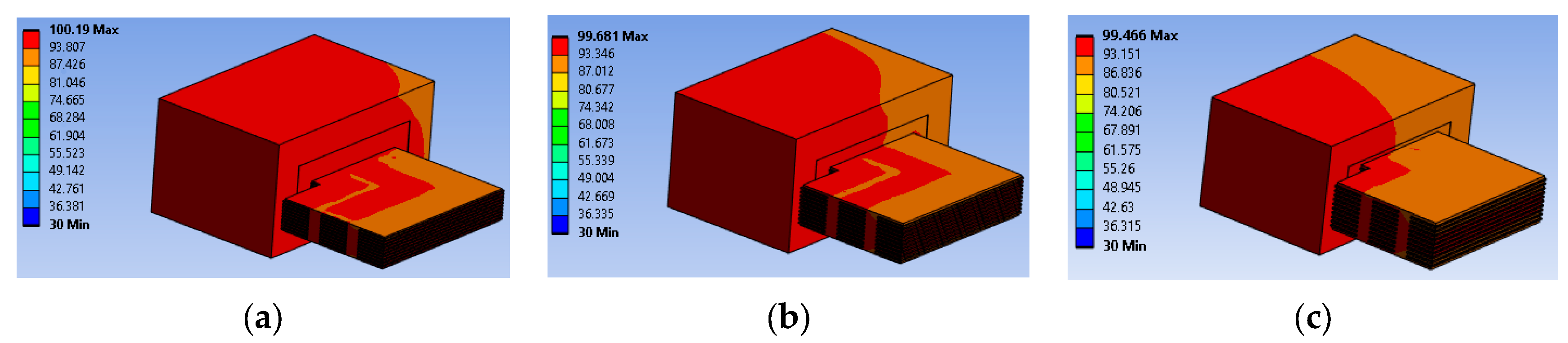
| Copper thickness (mm) | 0.2 | 0.2 | 0.2 |
| Insulator thickness (mm) | 0.2 | 0.3 | 0.4 |
| Transverse Kxy (W·m−2·K−1) | 190.1 | 152.1 | 126.8 |
| Normal Kz (W·m−2·K−1) | 0.30 | 0.25 | 0.22 |
| Maximal temperature (°C) | 100.19 | 99.68 | 99.46 |
| Parameters | Case 4 | Case 5 | Case 6 |
|---|---|---|---|
| Core losses (W) | 3 | 1.5 | 0 |
| Copper losses (W) | 0 | 1.5 | 3 |
| Maximal temperature (°C) | 102.7 | 100.2 | 104.56 |
| (°C) | 72.7 | 70.2 | 74.6 |
| (°C/W) | 6.1 | 5.9 | 6.2 |
| Error (%) | 3.6 | 0 | 6.2 |
| Application Note/Authors | Reference | Rth Model | Parameters |
|---|---|---|---|
| Magnetic Designer/Muldoon | [8,9] | External area—Aext | |
| Ferroxcube application note | [10] | Effective volume—Ve | |
| Ferroxcube Soft Ferrite Design Tool (SFDT) | [11] | Effective volume—Ve | |
| Hurley, Wölfe | [12] | Effective volume—Ve | |
| Van den Bossche, Valchev | [13] | External area—Aext Losses in the component—Pd | |
| McLyman | [14] | External area—Aext Losses in the component—Pd | |
| Zhang, Ngo | [2] | External area—Aext Losses in the component—Pd |
| E/PLT Core | Pmax | EE Core | Pmax |
|---|---|---|---|
| E/PLT32 | 4 | EE32 | 6 |
| E/PLT38 | 6 | EE38 | 7 |
| E/PLT43 | 7 | EE43 | 9 |
| E/PLT58 | 13 | EE58 | 16 |
| E/PLT64 | 17 | EE64 | 19 |
| Size | a3 | a2 | a1 | b | c |
|---|---|---|---|---|---|
| E/PLT32 | −0.0785 | 0.8908 | −4.379 | −0.0744 | 28.943 |
| E/PLT38 | −0.0232 | 0.3585 | −2.306 | −0.0527 | 18.942 |
| E/PLT43 | −0.0129 | 0.225 | −1.618 | −0.0437 | 16.019 |
| E/PLT58 | −0.00164 | 0.0486 | −0.5765 | −0.0268 | 9.335 |
| E/PLT64 | −0.00066 | 0.0251 | −0.3761 | −0.0219 | 7.558 |
| Size | a3 | a2 | a1 | b | c |
|---|---|---|---|---|---|
| EE32 | −0.0317 | 0.4889 | −3.125 | −0.0604 | 24.815 |
| EE38 | −0.0146 | 0.2537 | −1.8109 | −0.0448 | 17.146 |
| EE43 | −0.00642 | 0.1376 | −1.189 | −0.036 | 13.563 |
| EE58 | −0.00087 | 0.0309 | −0.4331 | −0.0223 | 7.977 |
| EE64 | −0.00045 | 0.0191 | −0.312 | −0.0192 | 6.7406 |
Disclaimer/Publisher’s Note: The statements, opinions and data contained in all publications are solely those of the individual author(s) and contributor(s) and not of MDPI and/or the editor(s). MDPI and/or the editor(s) disclaim responsibility for any injury to people or property resulting from any ideas, methods, instructions or products referred to in the content. |
© 2024 by the authors. Licensee MDPI, Basel, Switzerland. This article is an open access article distributed under the terms and conditions of the Creative Commons Attribution (CC BY) license (https://creativecommons.org/licenses/by/4.0/).
Share and Cite
Bakri, R.; Margueron, X.; Le Moigne, P.; Idir, N. Thermal Resistance Modeling for the Optimal Design of EE and E/PLT Core-Based Planar Magnetics. Energies 2024, 17, 2755. https://doi.org/10.3390/en17112755
Bakri R, Margueron X, Le Moigne P, Idir N. Thermal Resistance Modeling for the Optimal Design of EE and E/PLT Core-Based Planar Magnetics. Energies. 2024; 17(11):2755. https://doi.org/10.3390/en17112755
Chicago/Turabian StyleBakri, Reda, Xavier Margueron, Philippe Le Moigne, and Nadir Idir. 2024. "Thermal Resistance Modeling for the Optimal Design of EE and E/PLT Core-Based Planar Magnetics" Energies 17, no. 11: 2755. https://doi.org/10.3390/en17112755