Abstract
The reactive power optimization of an active distribution network can effectively deal with the problem of voltage overflows at some nodes caused by the integration of a high proportion of distributed sources into the distribution network. Aiming to address the limitations in previous studies of dynamic reactive power optimization using the cluster partitioning method, a three-stage dynamic reactive power optimization decoupling strategy for active distribution networks considering carbon emissions is proposed in this paper. First, a carbon emission index is proposed based on the carbon emission intensity, and a dynamic reactive power optimization mathematical model of an active distribution network is established with the minimum active power network loss, voltage deviation, and carbon emissions as the satisfaction objective functions. Second, in order to satisfy the requirement for the all-day motion times of discrete devices, a three-stage dynamic reactive power optimization decoupling strategy based on the partitioning around a medoids clustering algorithm is proposed. Finally, taking the improved IEEE33 and PG&E69-node distribution network systems as examples, the proposed linear decreasing mutation particle swarm optimization algorithm was used to solve the mathematical model. The results show that all the indicators of the proposed strategy and algorithm throughout the day are lower than those of other methods, which verifies the effectiveness of the proposed strategy and algorithm.
1. Introduction
In the 21st century, as China’s economy has grown and its people’s living standards have improved, the problem of energy shortages has become more serious. To deal with the problems of resource shortage and environmental pollution, the implementation of clean energy transmission and distribution control industry strategies has become the key decision in China’s economic development [1]. Therefore, the distributed generation (DG) supply represented by wind turbines (WTs) and photovoltaic (PV) power generation devices has been rapidly developed [2]. However, as a high proportion of DG is connected to the distribution network, it changes from a “passive network” to an “active network”. The randomness and uncertainty of its output, combined with multiple types of load volatility, will cause voltage control risks and problems such as feeder voltage overreach, which will pose huge challenges to the optimization control, safe operation, and operation situation prediction of the distribution network [3]. The reactive power optimization of the active distribution network is achieved by scheduling and adjusting reactive power control devices, such as the on-load voltage changer (OLTC), shunt capacitor bank (SCB), and static var compensator (SVC), which are effective means to ensure the economic and safe operation of the distribution network to achieve the goal of reducing active power network loss and improving system voltage quality [4].
Static reactive power optimization is the optimization of the landscape load of a section at a certain time. However, the wind-borne load is constantly changing throughout the day, which will lead to the frequent operation of discrete devices, such as the OLTC and SCB, thus shortening their service life, so this is not allowed in practical engineering applications [5]. Therefore, dynamic reactive power optimization is required to constrain the adjustment times of equipment throughout the day. However, in addition to the strong coupling of reactive power outputs between different periods of the day, the reactive power outputs of discrete devices, such as OLTC gear adjustment and the SCB, are also discrete. Therefore, the dynamic reactive power optimization of active distribution networks is a mixed-integer nonlinear programming (MINLP) problem, which is very difficult to solve directly [6].
In recent years, many scholars at home and abroad have explored the dynamic reactive power optimization problem of active distribution networks. Many scholars have studied the objective functions of optimization models. The authors of [4,7,8,9,10] established distribution network reactive power optimization mathematical models with the minimum active power loss as the objective function. They only considered the economy of the distribution network when establishing the mathematical model of reactive power optimization. Reference [11] established a mathematical model of the reactive power optimization of a distribution network with the minimum voltage deviation as the objective function. The authors only considered the safety of the distribution network when establishing the mathematical model of the reactive power optimization of the distribution network. On this basis, the authors of [12,13,14,15,16,17,18] considered the economy and safety of distribution network operation at the same time and established a reactive power optimization model for a distribution network with the minimum active network loss and voltage deviation/static voltage stability as the objective functions. The authors of [19] performed a more in-depth study on the operation economy of the distribution network. They established a multi-objective reactive power optimization model for a distribution network with the minimum investment in active power network loss, voltage deviation, and reactive power compensation devices. In order to constrain the adjustment times of control equipment throughout the day, the authors of [20,21] established a two-stage reactive power opportunity-constrained optimization model, with the objective functions being the minimum active power network loss and control equipment adjustment. In the same literature [22], in order to reduce the number of daily operations of discrete devices on a long time scale, an optimization model of discrete regulation equipment was established with the minimum active network loss, OLTC operation cost, and SCB operation cost as the objective functions, and a continuous regulation equipment optimization model with the minimum active network loss and voltage overcrossing risk as the objective functions was established for the short time scale. In [23], in order to prevent voltage overtripping, an optimization model with the minimum voltage overtripping severity, active power network loss, and voltage deviation as objective functions was established. Ref. [24] considered the problem of three-phase imbalance and established a three-phase distribution network voltage reactive power control model with the minimum voltage offset of each phase, active network loss, and three-phase imbalance of the local bus voltage as objective functions. Ref. [25] considered the reliability of photovoltaic power supply and established a reactive power optimization model with the minimum active network loss, an active power reduction in photovoltaic power supply, and the maximum junction temperature of IGBT as objective functions. In [26], electric vehicles were added to traditional new energy forms, and a reactive power optimization model was established with the minimum active power network loss, voltage deviation, and maximum static voltage stability margin as objective functions. The authors of [6] considered the harmonic distortion of wind turbines and established a reactive power optimization model with the minimum active power network loss, voltage deviation, OLTC operand, and harmonic distortion rate of wind turbines as objective functions. To achieve an economical operation in the context of the voltage/var optimization (VVO) problem while considering the stochastic bidirectional penetration of plug-in electric vehicles (PEVs), the authors of [27] established a reactive power optimization model aimed at minimizing the upstream network energy loss, minimizing the PEV charging cost, and minimizing the PV system input cost. However, in the context of the current dual “carbon neutral, carbon peak” strategy, none of the above studies considered the carbon emissions generated by -DG in the reactive power optimization process.
At the same time, some scholars have carried out research on how to reduce the maximum number of movements of discrete devices throughout the day during optimization, which can be roughly divided into the following categories: commercial solver methods [4], cost function methods [6,20,21,22], grey relational analysis methods [14], and cluster division methods [9,19,23]. There are some limitations in previous research on dynamic reactive power optimization using clustering partition methods: (1) The K-Means clustering algorithm uses the average value as the cluster center, which is not in line with the actual situation. (2) The computational steps of the Ward clustering algorithm are complex. (3) At present, the optimal value adjustment rule of discrete control equipment only uses the average value instead, which is too simple to lead to a large difference between the actual value that meets adjustment requirements and the optimal value, thus reducing the dynamic reactive power optimization effect.
This paper presents three major contributions to the field of reactive power optimization of active distribution networks:
- (1)
- In the current dual carbon context, this paper optimizes the carbon emission index of DG as one of the objective functions of the reactive power optimization mathematical model of an active distribution network.
- (2)
- In view of the limitations existing in previous research on dynamic reactive power optimization based on the clustering partition method, a three-stage dynamic reactive power optimization decoupling strategy for an active distribution network based on the partitioning around medoids (PAM) clustering algorithm is proposed.
- (3)
- The standard particle swarm optimization algorithm easily falls into local optima when solving optimal power flow problems, such as the reactive power optimization of an active distribution network. This paper proposes a linear decreasing mutation particle swarm optimization algorithm to solve the mathematical model.
The subsequent sections of this paper are structured as follows. Section 2 shows the dynamic reactive power optimization mathematical model of an active distribution network composed of objective functions and constraint conditions. Section 3 shows the linear decreasing mutation particle swarm optimization algorithm used to solve the model. Section 4 shows the proposed three-stage decoupling strategy for an active distribution network’s dynamic reactive power optimization based on the PAM clustering algorithm in this paper. Section 5 demonstrates the superiority of the proposed strategy and algorithm through numerical examples. Section 6 summarizes the research work in this paper and explores future research directions.
2. Dynamic Reactive Power Optimization Mathematical Model of Active Distribution Network
2.1. Objective Functions
The goal of reactive power optimization should consider the economy, security, and low carbon of the distribution network [28]. In this paper, the minimum active power network loss, voltage deviation, and carbon emissions are used as sub-objective functions to establish the satisfaction function model.
- (1)
- Minimum active network loss
In (1), is the system’s active power network loss; and are the voltage amplitudes of node i and node j, respectively; and are, respectively, the real and imaginary elements of the bus admittance matrix between node i and node j; and m indicates the total number of branches.
- (2)
- Minimum voltage deviation
In (2), is the system voltage deviation; is the actual voltage of node j; is the rated voltage of node j; and n indicates the total number of nodes.
- (3)
- Minimum carbon emissions
In the current dual carbon context, considering the carbon emissions of power generation energy is crucial and is a response to the national call. Therefore, this paper takes the minimum DG carbon emissions as one of the optimization objectives.
Based on the life-cycle assessment method, this paper analyzes the carbon footprint of WT and PV units, obtains the unit carbon emission intensity by combining materials, energy consumption, and carbon emission factors of different links [29], and proposes the DG carbon emission index.
In (3), is the total carbon emissions of DG; and are the sets of WT and PV access nodes in the distribution network; and are the unit carbon emission intensities of WT and PV units, respectively; and and are the active output absorption of WT and PV units at node i, respectively.
In this paper, a single-objective reactive power optimization mathematical model is established to explore the impact of optimizing a single objective on the other objectives. The PSO algorithm is used to solve the model. The improved IEEE33-node distribution network [30] is used for a calculation example.
As can be seen from Table 1, performing single-objective reactive power optimization is bound to weaken the optimization degree of the other objectives, so it is necessary to consider the reactive power optimization model in the form of multi-objective weighted summation at the same time.

Table 1.
Comparison results of all-day reactive power optimization effect.
Since the units of the three objective functions are different, they are normalized and weighted together in the satisfaction function.
In (4) and (5), F is the satisfaction function, and the closer the value is to 1, the better the reactive power optimization effect is; is the normalized objective function, where ; is the original objective function, where ; is the result without reactive power optimization; is the result of single-objective reactive power optimization; and is the corresponding weight coefficient of each objective function, where , since the main objective of the dynamic reactive power optimization of an active distribution network is to reduce the active power of the system, and the secondary objective is to improve the quality of the system voltage, so the value is divided according to importance by the analytic hierarchy process [31]: active network loss > voltage deviation > carbon emissions. This results in , , and .
2.2. Constraint Conditions
- (1)
- Power flow equation constraints
In (6) and (7), and are the active and reactive power injected by the generator and DG, respectively; and are the active and reactive power consumed by the load, respectively; is the reactive power compensated by node i; and and are the conductance and susceptance between node i and node j.
- (2)
- Node voltage constraints
In (8), is the voltage amplitude of node i; and are the upper limit and lower limit of the node voltage amplitude.
- (3)
- Equilibrium node constraints
In (9) and (10), and are the lower limit and upper limit of active power of the equilibrium node, respectively; is the active power inflow from the transmission system operator (TSO); and are the lower limit and upper limit of reactive power of the equilibrium node, respectively; and is the reactive power inflow from the TSO.
- (4)
- OLTC gear constraints
In (11), K indicates the OLTC gear value; and are the maximum and minimum levels of the OLTC, respectively.
- (5)
- Constraints on the maximum number of OLTC adjustments throughout the day
In (12), is the gear value of the OLTC at the moment; indicates the maximum number of OLTC adjustments in an entire day.
- (6)
- Reactive power output constraint of reactive power compensation device
In (13) and (14), is the reactive power output of the SVC; and are the upper limit and lower limit of the SVC reactive power output, respectively; is the reactive power output of the SCB; and are the upper limit and lower limit of the reactive power output of the SCB.
- (7)
- SCB’s maximum number of daily switching constraints
In (15), is the reactive power output of the SCB in time; ⨁ is the xOR operator; and indicates the maximum number of SCB switches in a whole day. If the reactive power output of the SCB changes at the hour, ; if the reactive power output of the SCB does not change at the hour, .
- (8)
- Restriction of DG output cutting quantity
To simplify the calculation, the and are treated as PQ-type DG connected to the distribution network in this paper. The output of DG will not be fully absorbed when it is connected to the distribution network at certain times. Therefore, to make the optimization model conform to the actual situation, the restriction on the and spillage is adopted as one of the constraints of the optimization model.
In (16), is the active output cutting quantity of the jth ; and are the upper and lower limits of active output cuts, respectively. In (17), is the reactive output cutting quantity of the jth ; and are the upper and lower limits of reactive output cuts, respectively. In (18), is the active output cutting quantity of the jth ; and are the upper and lower limits of active output cuts, respectively. In (19), is the reactive output cutting quantity of the jth ; and are the upper and lower limits of reactive output cuts, respectively.
3. Linear Decreasing Mutation Particle Swarm Optimization
The idea of particle swarm optimization comes from research on the foraging behavior of birds, whereby the group finds the optimal destination through collective information sharing [32].
The standard particle swarm optimization algorithm uses a particle population to optimize the objective function, which has a fast operation speed and few structural parameters, so it is widely used in the research of the dynamic reactive power optimization of active distribution networks [16,19,33]. But it easily falls into the local optimal solution. Therefore, in order to improve the solution accuracy of the algorithm, this paper proposes a linear decreasing mutation particle swarm optimization (LDMPSO) algorithm, and the specific steps are as follows:
- (1)
- In order to make the particle population search more thorough, the inertia weight w is improved in the form of a linear decrease [34].
In (20), w is the inertia weight; and are the upper and lower limits of the inertia weight, respectively; is the number of current iterations; and indicates the maximum number of iterations.
In the early stage of iteration, the large inertia weight leads the particle swarm to find the optimal solution in the global scope. In the late iteration, the small inertia weight leads the particle swarm to find the optimal solution in the local scope.
- (2)
- In order to improve the convergence speed of the population, this paper improves the individual learning factor and social learning factor .
In (21) and (22), is an individual learning factor; and are the upper and lower limits of individual learning factors, respectively; is a social learning factor; and and are the upper and lower limits of social learning factors, respectively.
- (3)
- In order to improve the overall convergence accuracy of the population, the population particles are arranged in ascending order according to the fitness value at each iteration. The last 20% of particles are randomly learned from the historical best position of one of the first 20%.
In (23), is the position of particle i in generation k + 1; is the position of particle i in generation k; is the individual optimal position of a certain particle located in the top 20% of generation k; and is the global optimal position of the kth-generation particle.
- (4)
- In order to prevent the population from falling into the local optimal solution during the iterative search, this paper randomly selected 10% of the population to mutate when the fitness value of the global optimal particle did not change for five consecutive iterations.
In (24), Z is the coefficient of variation, and the range of values is (0.3, 0.7); the value is taken randomly in each iteration.
The pseudocode of the proposed LDMPSO Algorithm 1 is as follows.
| Algorithm 1 LDMPSO algorithm. |
|
4. Three-Stage Dynamic Reactive Power Optimization Decoupling Strategy for Active Distribution Network
Aiming to solve the MINLP problem of the dynamic reactive power optimization of an active distribution network, this paper first adopts a discrete method followed by a continuous method to implement three-stage decoupling to obtain the global optimal solution.
The core of the three-stage dynamic reactive power optimization decoupling strategy for active distribution networks in the second stage is to convert the optimal action values of the discrete devices to the actual action values. The specific steps are as follows.
The optimal all-day gear values/compensation values of the OLTC and SCB are taken as the sample set, and the PAM clustering of the samples is performed as follows:
- (1)
- Randomly select data as the initial clustering center point.
- (2)
- Calculate the distance between the data of each noncentral point and the central point of each cluster.
- (3)
- Assign the sample of each noncentral point to the group represented by the nearest central point, and calculate the sum of absolute errors E.
In (25), E is the sum of absolute errors; is sample i; is the central point of the group; and n is the number of samples in the group.
- (4)
- Randomly select a sample with a noncentral point to replace the central point of a certain group, and calculate the sum of absolute errors E again.
- (5)
- Calculate the sum of absolute error differences before and after substitution . If , use the sample as the center point of the group; otherwise, do not change it.
- (6)
- Repeat (4)∼(5) until the center point is no longer changed.
- (7)
- After clustering is completed, add the category number of the group to which each sample belongs.
The one-time adjustment rule is as follows: if the sample has m consecutive hours belonging to the same group, the m hours are merged into a period, and the gear value/ compensation value of the period after fusion is as follows:
- (1)
- If , all values in that period are replaced by the mean.
- (2)
- If , if there are two different values, all values in the period are replaced by the value that occurs more often; if there are three different values, all values in the period are replaced by the median; and if there are four or more different values, all values in the period are replaced by the mean.
After one adjustment, the second phase ends if the discrete device has reached the maximum number of adjustments/switches in the whole day; otherwise, the second adjustment is performed.
For the OLTC, the secondary adjustment rules are as follows:
- (1)
- If there is one sample in the period, the sample value of the period is
In (26), is the sample value in the period; is the sample in the period after the second adjustment.
If the sample value in the last period in one day is the same as the sample value in the initial period, the sample value in the last period of that day is
- (2)
- If there are two or more samples in the period, the sample value in the period remains unchanged.
The second adjustment is repeated until the maximum number of adjustments/switches for the day is reached.
- (3)
- If the maximum number of actions in the whole day still cannot be reached after many repeated adjustments, the sample value of two or fewer samples in the period is
For the SCB, the secondary adjustment rules are as follows:
- (1)
- If there is one sample in the period, the sample value in the period is
If the sample value in the last period in one day is the same as the sample value in the initial period, the sample value in the last period of that day is
- (2)
- If there are two or more samples in the period, the sample value in the period remains unchanged.
The second adjustment is repeated until the maximum number of adjustments/switches for the day is reached.
- (3)
- If the maximum number of actions in the whole day still cannot be reached after many repeated adjustments, the sample value of two or fewer samples in the period is
Compared with the current dynamic reactive power optimization research based on the clustering partition method, the proposed method has the following advantages:
- (1)
- The PAM clustering algorithm uses the actual value instead of the average value as the cluster center, which is more in line with the actual operation of reactive power optimization of an active distribution network, and the calculation steps are relatively simple.
- (2)
- It uses more detailed optimal value adjustment rules for discrete equipment, which has a better dynamic reactive power optimization effect than the direct simple adjustment of the average value.
The performance of convergence characteristics determines the quality of clustering algorithms. In order to prove the effectiveness of the PAM clustering algorithm in dealing with the reactive power optimization-related clustering problem for an active distribution network, this paper uses the improved PG&E69-node distribution network [35] as a case to compare different clustering algorithms (Table 2 and Table 3). Due to the randomness of the cluster center selection, each clustering algorithm is run 5 times.
Table 2.
Comparison of convergence characteristics of different clustering algorithms (OLTC).
Table 3.
Comparison of convergence characteristics of different clustering algorithms (SCB2).
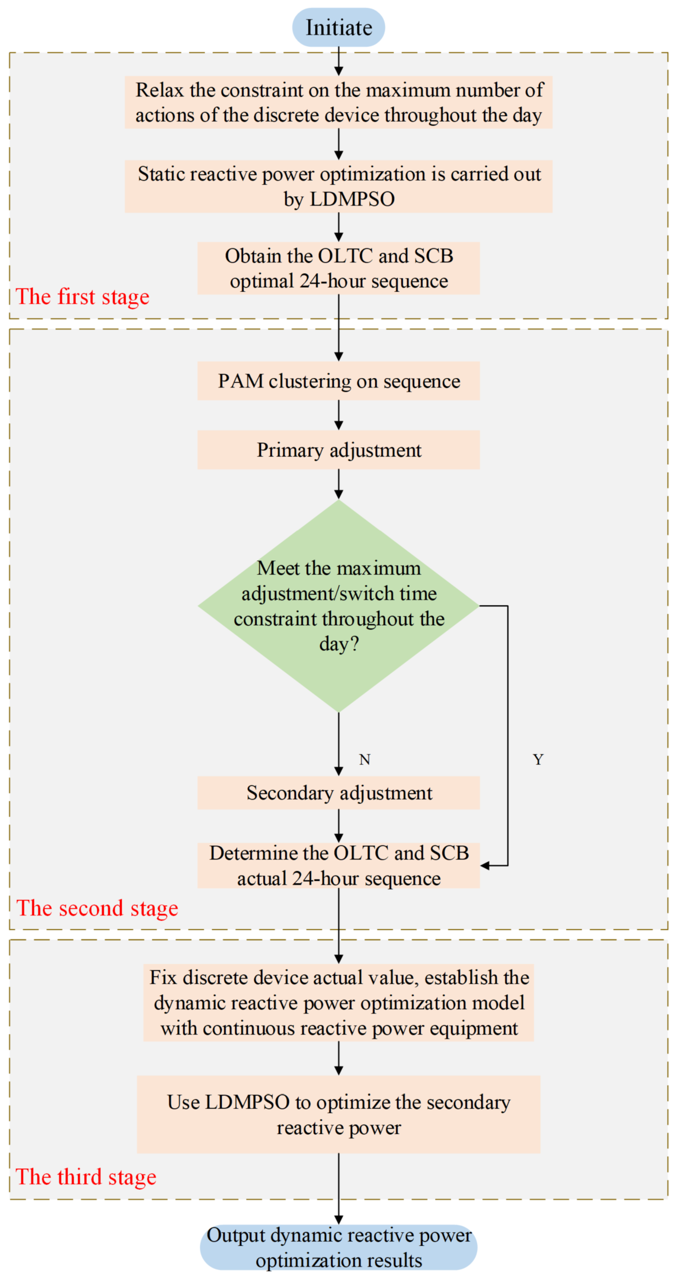
The three-stage dynamic reactive power optimization decoupling strategy flow chart for an active distribution network is shown in Figure 1.
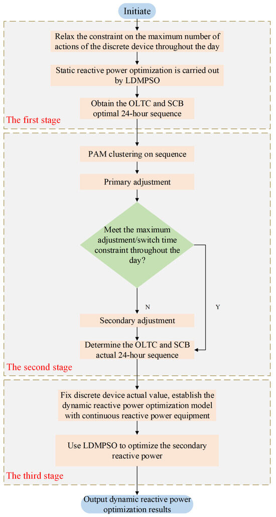
Figure 1.
Three-stage dynamic reactive power optimization decoupling strategy flow chart for active distribution network.
5. Example Analysis
5.1. Introduction of Numerical Examples
This paper is based on MATLAB software (2018 b) platform programming. Computer configuration: the CPU is i5-8250U, the main frequency is 1.6 GHz with 8GRAM, the graphics card is NVDIA GeForce MX 150, and the operating system is a Windows 10 64-bit operating system.
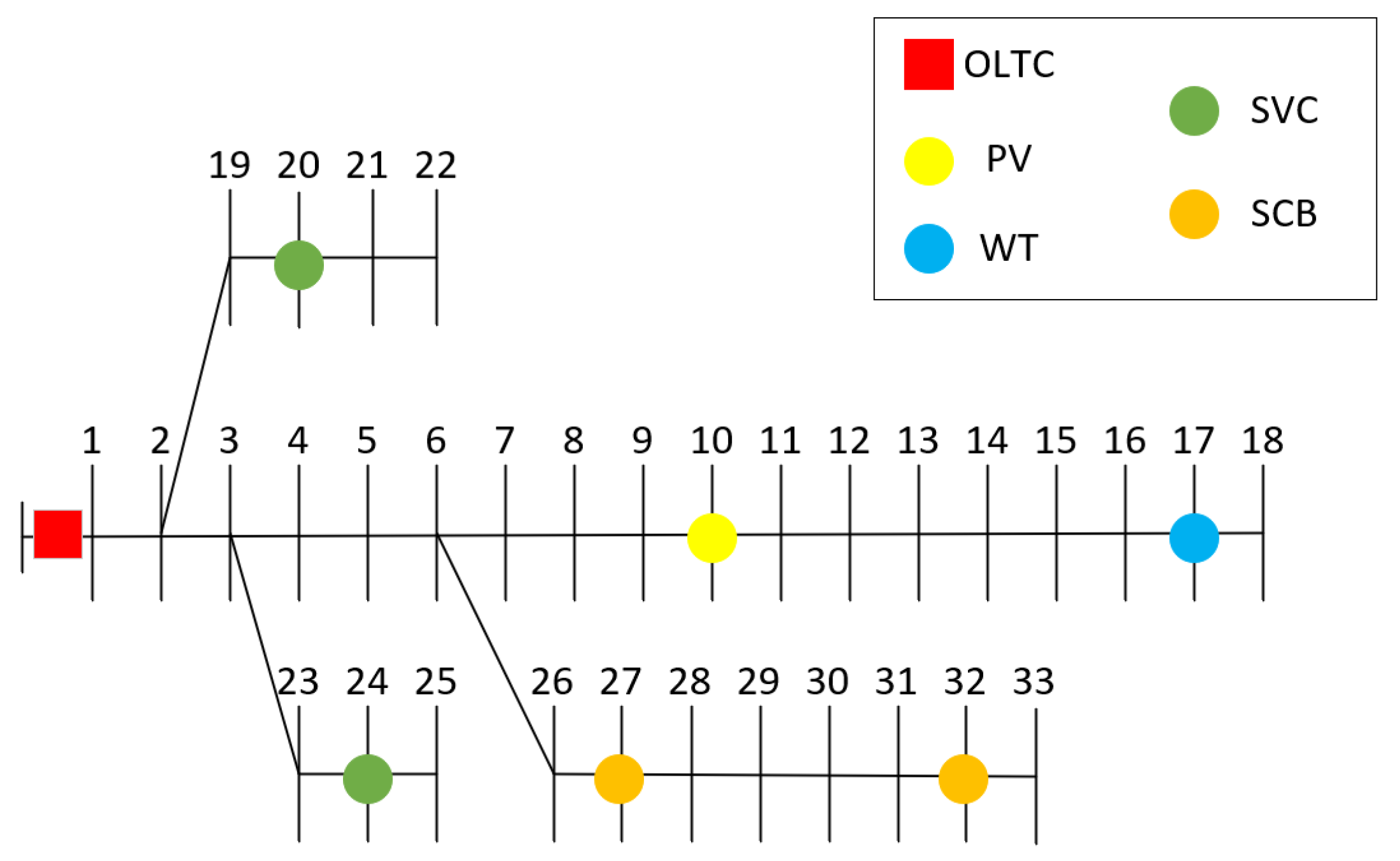
The improved IEEE33−node distribution network is adopted in the calculation example, as shown in Figure 2. The PV and WT units are connected to nodes 10 and 17, respectively, the capacity is 1 MW, the power factor is 0.95, and the WT and PV spillage is 0∼30% of the total. The balance node is connected to the OLTC, its adjustable voltage range is 0.95∼1.05 p.u., the adjustment step is 1.25%, and the total number of levels is 9. A total of 20 and 24 nodes are connected to SVC1 and SVC2, and the reactive power compensation capacity is 1 MVar; SCB1 and SCB2 are connected to 27 and 32 nodes, the reactive power compensation capacity of a single group is 50 kVar, and 20 groups are installed on each node. The maximum number of OLTC and SCB actions and in a day is 30 and 5, respectively; the base capacity is 10 MW, the reference voltage of the system is 12.66 kV, and a constant power load is adopted. The upper and lower limits of the per unit voltage of each node are set at 1.05 p.u. and 0.95 p.u., respectively, according to the medium-voltage distribution network (10 kV) standard.

Figure 2.
Improved IEEE33—node distribution network structure diagram.
At the same time, in order to test the performance of the proposed strategy and algorithm in a large-scale, complex distribution network, the improved PG&E69−node distribution network is taken as an example, as shown in Figure 3. The PV and WT units are connected to nodes 17 and 23, respectively; the balance node is connected to the OLTC; 32 and 63 nodes are connected to SVC1 and SVC2; and SCB1 and SCB2 are connected to 45 and 53 nodes. The parameter setting of the device is the same as that of the improved IEEE33-node distribution network. The base capacity is 10 MW, the reference voltage of the system is 12.66 kV, and a constant power load is adopted; the upper and lower limits of the per unit voltage of each node are set at 1.05 p.u. and 0.95 p.u., respectively, according to the medium-voltage distribution network (10 kV) standard.
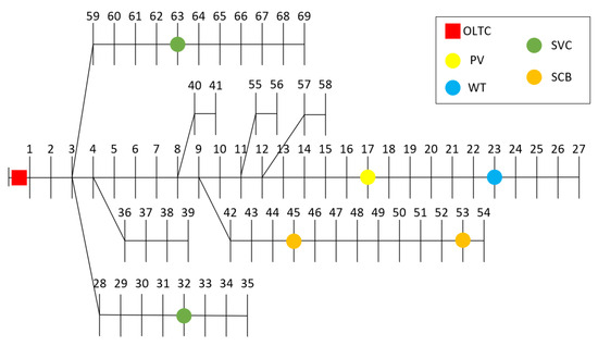
Figure 3.
Improved PG&E69—node distribution network structure diagram.
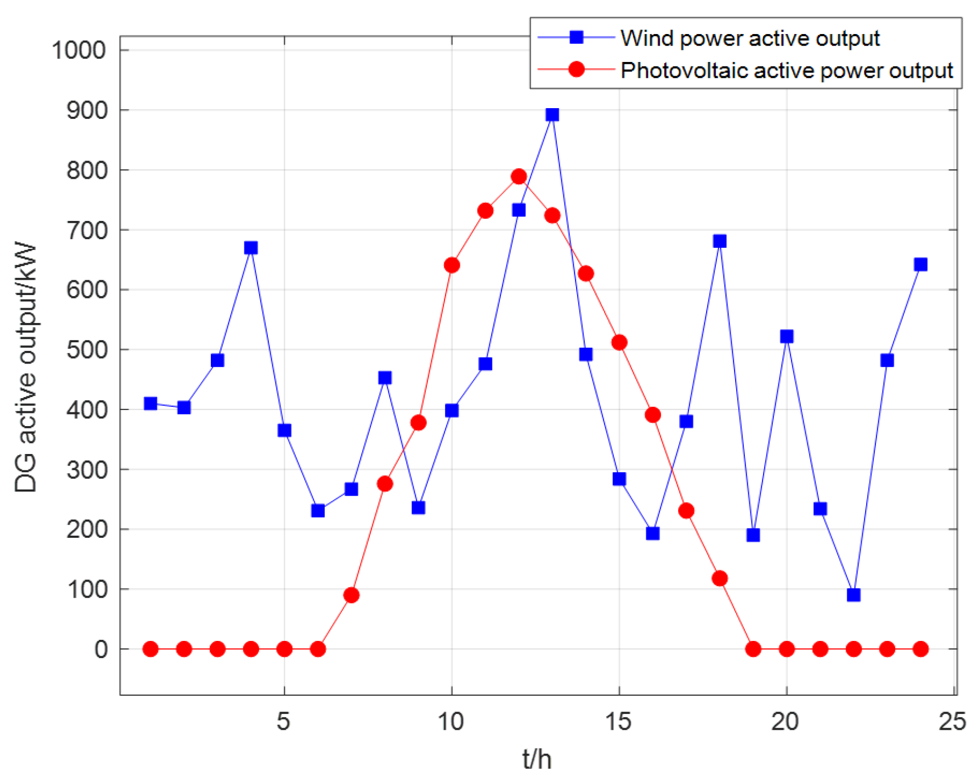
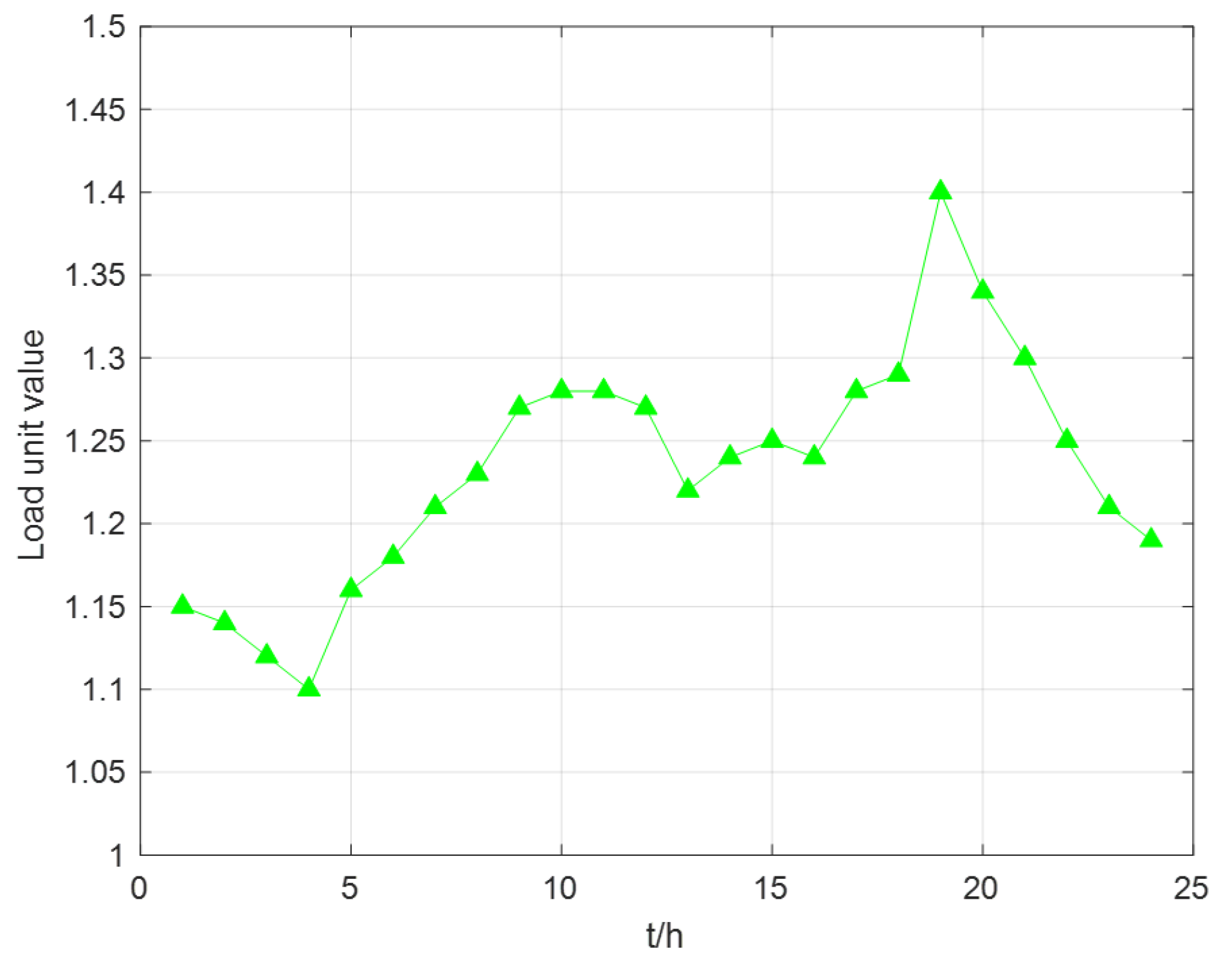
The unit carbon emission intensities of WT and PV units [29] are shown in Table 4; considering the uncertainty of DG output, based on the annual wind power generation and photovoltaic power generation data sets for a certain region in East China (1 h is one point), this paper first uses the Monte Carlo method to generate scenes and then uses a heuristic synchronous backtracking reduction method to reduce the scenes. The active power output curves of wind and photovoltaic power and the daily load curve of the conventional load are shown in Figure 4 and Figure 5.
Table 4.
Results of carbon emission intensity per unit of wind and solar power generation units.
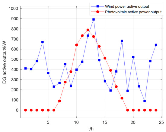
Figure 4.
All—day active power output curve of wind and photovoltaic power.
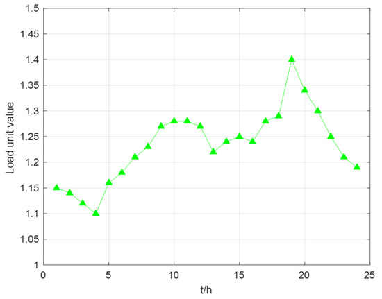
Figure 5.
Daily load curve of conventional load.
The three−stage dynamic reactive power optimization decoupling strategy for an active distribution network is used for reactive power optimization, and the forward and backward generation method is used for the power flow calculation.
5.2. Analysis of Dynamic Reactive Power Optimization Results
The LDMPSO algorithm was used to solve the model. It is very important to evaluate the variation in the LDMPSO algorithm parameters (, , , , , ) for the reactive power optimization effect.
As can be seen in Table 5 and Table 6, the reactive power optimization effect is best when is set to 0.8, and is set to 0.2; and are set to 2 and and are set to 0.5 in both examples.
Table 5.
Comparison of all-day reactive power optimization effects of different settings of LDMPSO algorithm-related parameters (improved IEEE33—node distribution network).
Table 6.
Comparison of all-day reactive power optimization effects of different settings of LDMPSO algorithm-related parameters (improved PG&E69—node distribution network).
Therefore, the LDMPSO algorithm parameters are set as follows: the population size is 50; the maximum iteration number is 100; is set to 0.8, and is set to 0.2; and are set to 2; and and are set to 0.5.
In order to reflect the advantages of the proposed strategy in the current dynamic reactive power optimization research based on the clustering partition method, five groups of controlled experiments were set up. Experiment 1 was conducted before reactive power optimization; experiment 2 applied static reactive power optimization (the relaxation of the maximum number of movements of the discrete device throughout the day); experiment 3 adopted the strategy based on the K-Means clustering algorithm proposed in [19]; experiment 4 adopted the strategy based on the Ward clustering algorithm proposed in [23]; and experiment 5 adopted the strategy based on the PAM clustering algorithm proposed in this paper.
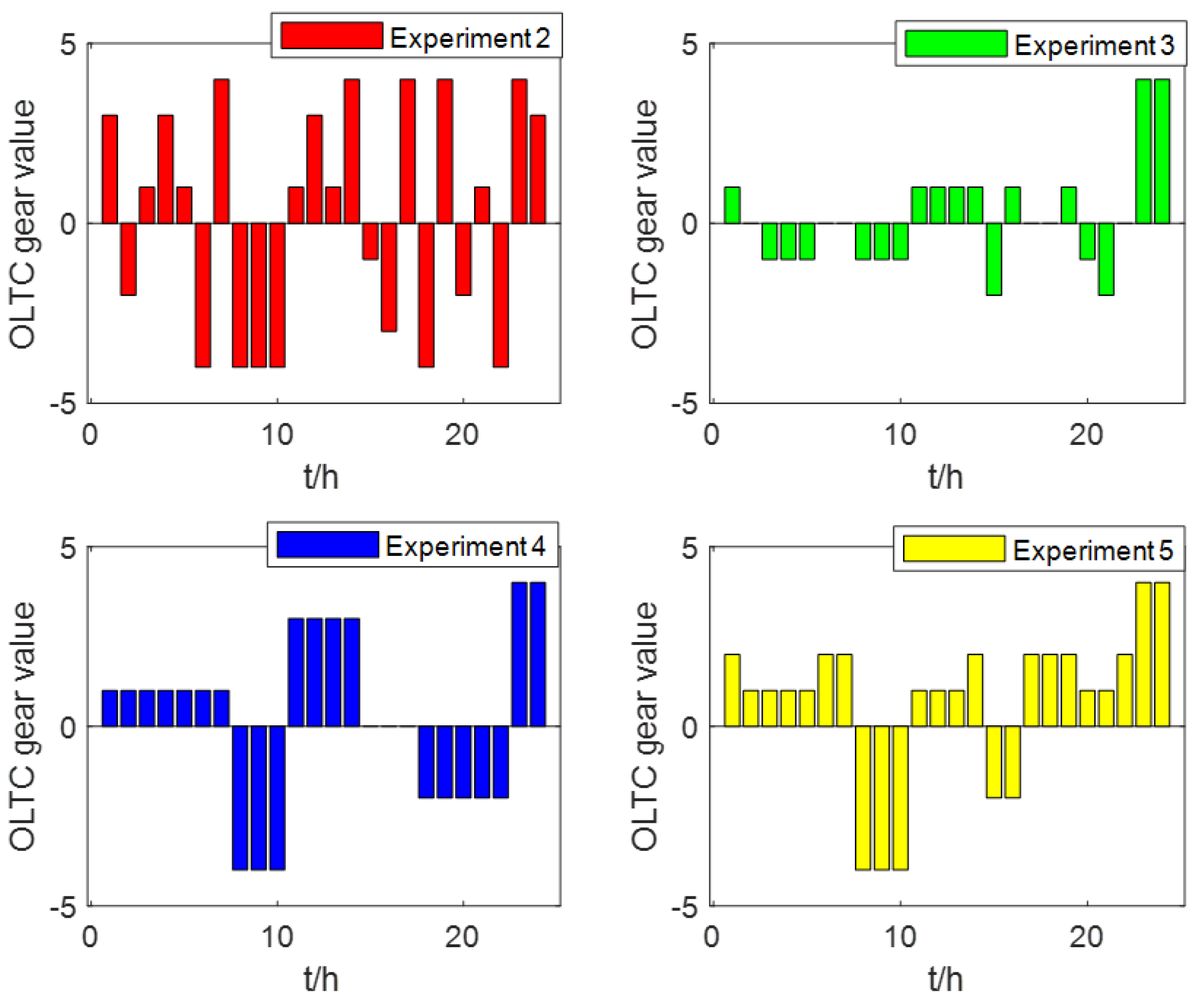
The improved IEEE33−node distribution network is illustrated as an example. The results of experiment 2 show that SCB2 already satisfies the constraint of maximum all-day switching times in the static reactive power optimization in the first stage, so the second and third stages are not necessary. Figure 6 and Figure 7 (Figure 8 and Figure 9) show the OLTC all-day gear and SCB1 all−day compensation capacity results for each group, respectively.
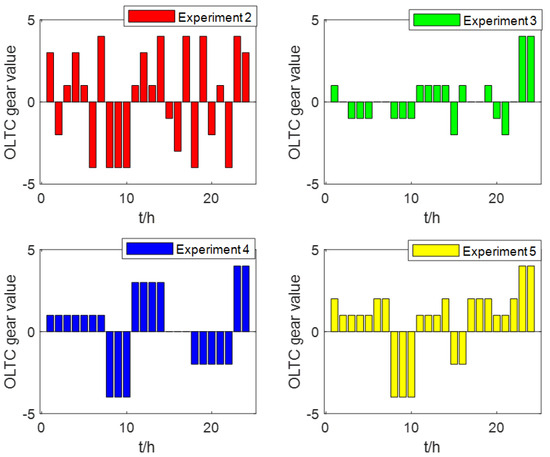
Figure 6.
OLTC all—day gear adjustment results (improved IEEE33—node distribution network).
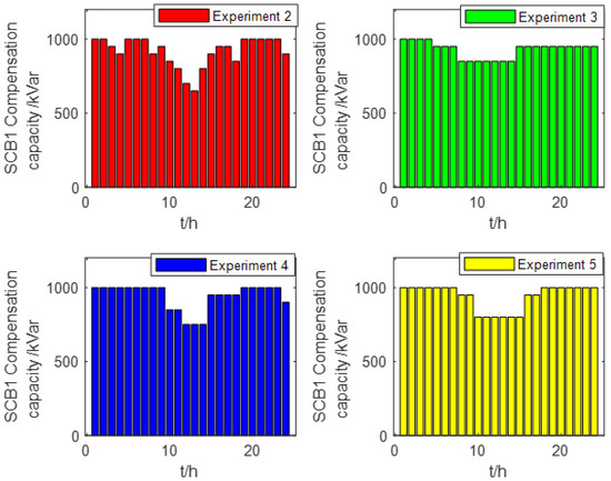
Figure 7.
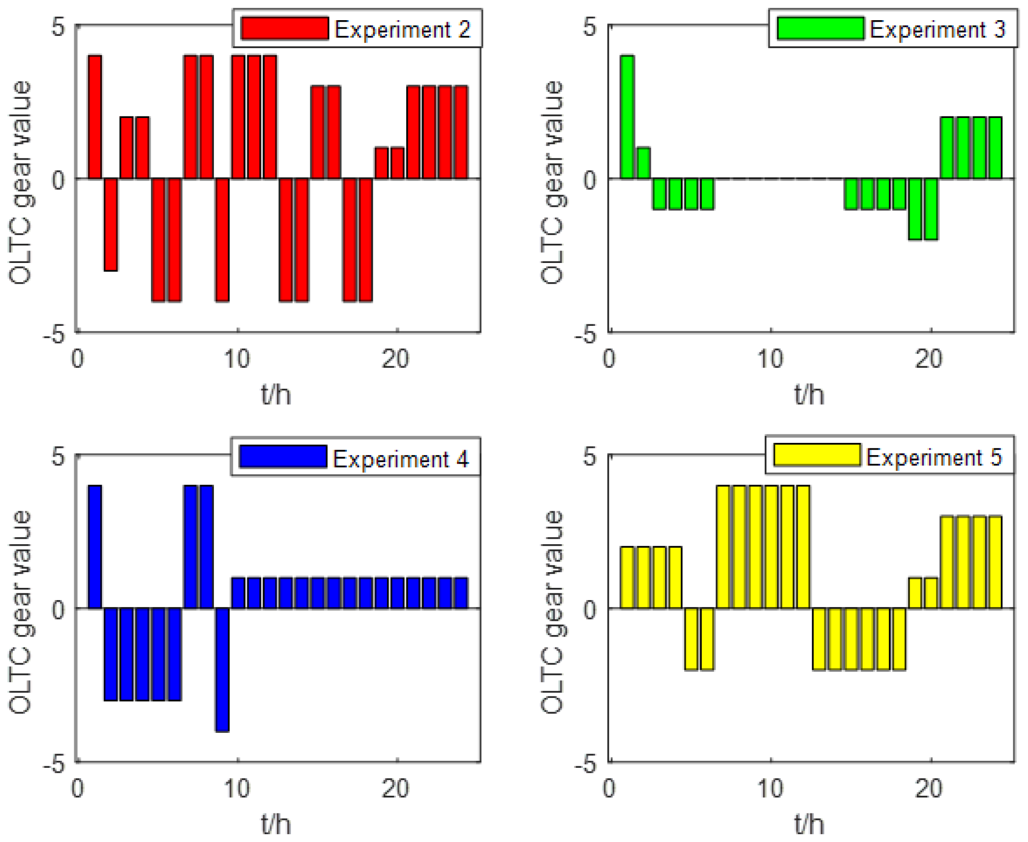
OLTC all—day gear adjustment results (improved PG&E69—node distribution network).

Figure 8.
SCB1 compensation capacity switching results throughout the day (improved IEEE33—node distribution network).
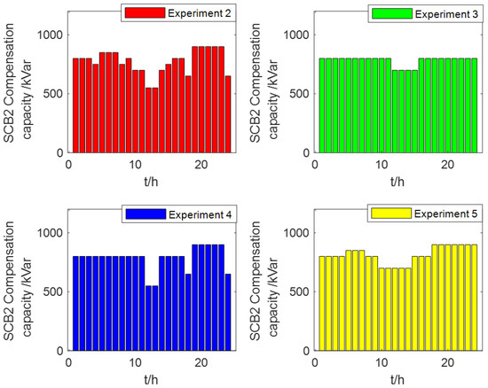
Figure 9.
SCB2 compensation capacity switching results throughout the day (improved PG&E69—node distribution network).
In order to more intuitively adjust/switch the effects of the OLTC and SCB1 using different strategies, the OLTC all-day gear deviation value and SCB all-day compensation capacity deviation rate are defined as follows:
In (32) and (33), is the actual gear value of the OLTC at the moment; is the optimal gear value of the OLTC at time; is the shift deviation of the OLTC for the whole day; is the actual compensation capacity value of SCB at time; is the optimal compensation capacity value of the SCB at time; and is the SCB all-day compensation capacity deviation rate. The smaller the OLTC all-day gear deviation value and the SCB all-day compensation capacity deviation rate, the closer the actual value of the discrete device in this strategy to the optimal value of static reactive power optimization without strong time coupling; thus, the rationality of this strategy can be reflected more effectively.
Table 7 and Table 8 (Table 9 and Table 10), respectively, show the results of the discrete equipment gear/compensation capacity deviation and the comparison results of the all-day reactive power optimization effect for each group of experiments. It can be seen in Table 7 that the all-day adjustment times of the OLTC and the all-day switching times of SCB1 in experiment 2 are 98 and 15 times, respectively, both of which exceed the specified maximum number of all-day movements, thus shortening their service life.
Table 7.
Discrete device deviation results for each group of experiments (improved IEEE33—node distribution network).
Table 8.
Discrete device deviation results for each group of experiments (improved PG&E69—node distribution network).
Table 9.
Comparison results of all-day reactive power optimization effect (improved IEEE33—node distribution network).
Table 10.
Comparison results of all-day reactive power optimization effect (improved PG&E69—node distribution network).
Experiments reduced the number of OLTC adjustments to 23 and 26; the number of SCB1 cuts throughout the day is reduced to 3, 5, and 4, which meets the requirements of the regulations. Compared with experiment 3, experiment 4 reduced the OLTC all-day gear deviation from 59 to 42; the compensation capacity deviation rate of SCB1 was reduced from 6.67% to 4.38%. This is because the strategy based on the K-Means clustering algorithm adopted in experiment 3 adopts the data mean to calculate the new cluster center, which is not in line with the actual situation; however, the strategy adopted in experiment 4 based on the Ward clustering algorithm turns to the method of calculating the sum of squares of deviations after combining two adjacent samples to classify each sample. However, it can be seen in Table 9 that experiment 3 reduced the all-day average active power network loss from 283.09 kW to 147.52 kW, a reduction percentage of 47.89%; the average voltage deviation for the whole day is reduced from 25.44 V to 13.54 kV, with a reduction percentage of 46.78%. But in experiment 4, the average daily active power network loss decreased from 283.09 kW to 147.94 kW, with a reduction percentage of 47.74%; the average voltage deviation for the whole day was reduced from 25.44 kV to 13.60 kV, a reduction of 46.54%. It can be seen that the strategy based on the Ward clustering algorithm adopted in experiment 4 reduces the deviation between the actual OLTC all-day gear and the actual SCB1 all-day compensation capacity and their optimal values to the greatest extent, but it ignores the improvement of the all-day average active power network loss and all-day average voltage deviation reduction.
The strategy based on the PAM clustering algorithm used in experiment 5 reduced the OLTC all-day gear deviation value from 59 in experiment 3 and 42 in experiment 4 to 40, and the compensation capacity deviation rate of SCB1 was reduced from 6.67% in experiment 3 and 4.38% in experiment 4 to 3.53%. This is because the strategy adopted in experiment 5 based on the PAM clustering algorithm is to randomly select data as the new cluster center, which is more in line with the actual situation than the strategy used in experiment 3.
The average all-day active power network loss decreased from 283.09 kW to 147.21 kW; the reduction rate increased from 47.89% in experiment 3 and 47.74% in experiment 4 to 48.00%. The average voltage deviation for the whole day was reduced from 25.44 kV to 13.53 kV, and the reduction range was increased from 46.78% in experiment 3 and 46.54% in experiment 4 to 46.82%. At the same time, it can be seen from the average daily carbon emissions in each group that, compared with experiment 3, experiment 4 only reduced it from 7859.3 g to 7852.8 g, while experiment 5 reduced it to 7838.1 g, with the reduction rate increasing from 8.3% to 27.0%. This is because the formulation of the optimal value adjustment rule for discrete devices in this paper is more detailed, which makes up for the shortcomings of the strategies used in experiments 3 and 4. Therefore, the effectiveness of the proposed strategy is verified.
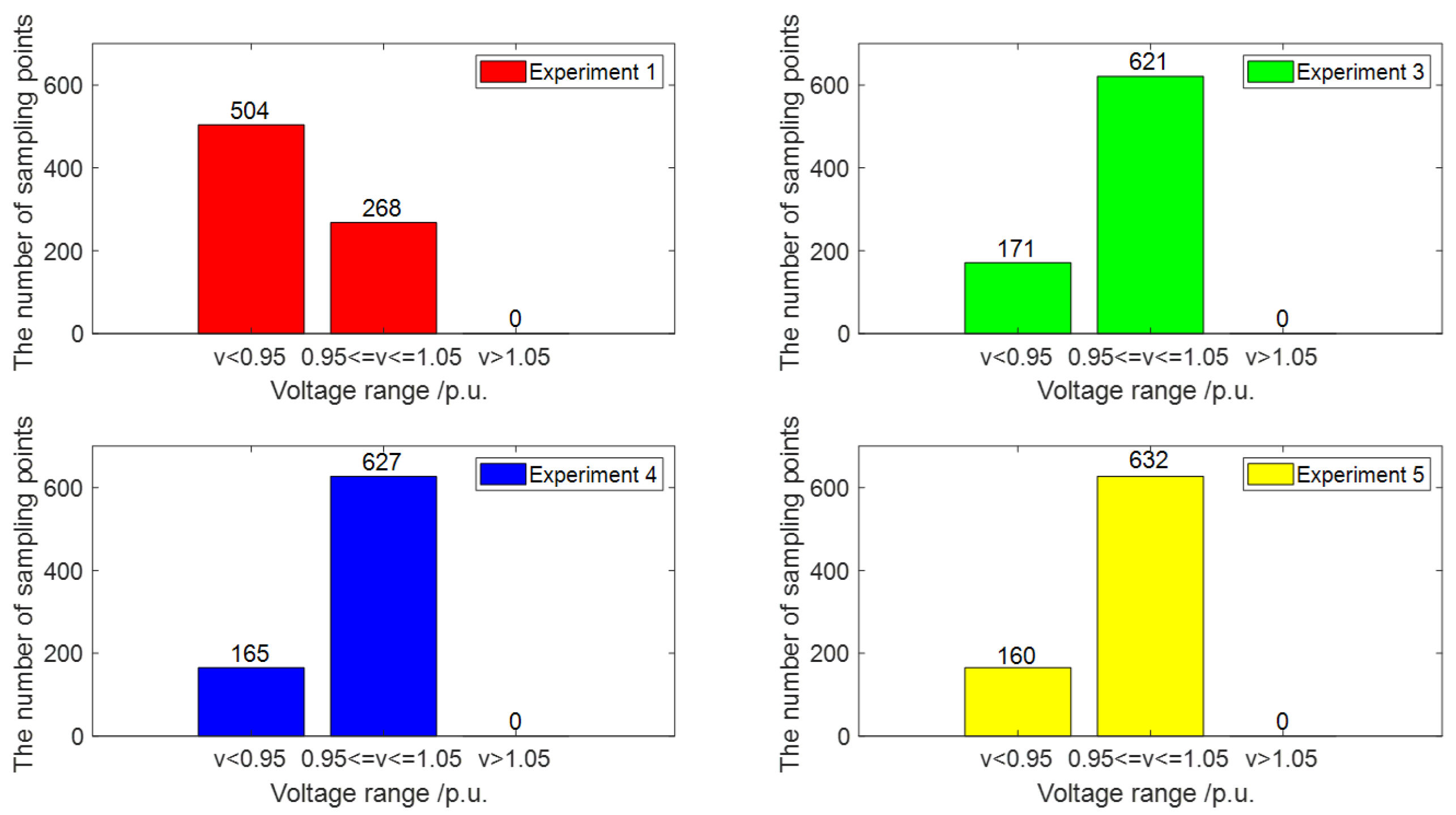
Figure 10 shows the statistical plot of the node voltage at 24 × 33 sampling points throughout the day for each experiment. The number 24 represents 24 h in a day, and 33 represents the number of nodes in the distribution network. A node voltage less than 0.95 p.u. or greater than 1.05 p.u. indicates that the voltage is out of limit.

Figure 10.
Statistical plots of system node voltages in different experiments (improved IEEE33—node distribution network).
As can be seen in Figure 10 (Figure 11), the all-day dynamic reactive power optimization obtained with the proposed strategy in experiment 5 performs the best in terms of reducing out-of-limit voltage at the system nodes.
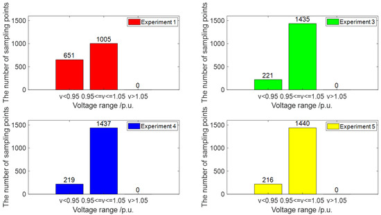
Figure 11.
Statistical plots of system node voltages in different experiments (improved PG&E69-node distribution network).
In order to prove the superiority of the proposed algorithm in dealing with the optimal power flow problem, five groups of experiments were designed under the condition of relaxing the maximum number of actions of the discrete device for the whole day. Experiment 1 was conducted before reactive power optimization; experiment 2 applied reactive power optimization using PSO; experiment 3 applied reactive power optimization using CBPSO [36]; experiment 4 applied reactive power optimization using DCPSO [37]; and experiment 5 applied reactive power optimization using the LDMPSO algorithm proposed in this paper. Due to the randomness of the population particle’s initial position, this study ran each experiment five times, and the results were averaged.
The improved IEEE33-node distribution network is illustrated as an example. Table 11 (Table 12) shows that the LDMPSO algorithm proposed in this paper has the best performance: the average active power network loss for the whole day was reduced from 283.09 kW to 132.28 kW, and the reduction percentage was increased from 47.19% with the PSO algorithm, 47.57% with the CBPSO algorithm, and 49.06% with the DCPSO algorithm to 53.27%. The average voltage deviation for the whole system was reduced from 25.44 kV to 12.53 kV, and the reduction percentage was increased from 45.48% with the PSO algorithm, 46.78% with the CBPSO algorithm, and 50.67% with the DCPSO algorithm to 50.75%. The average carbon emissions for the whole day also performed the best. Therefore, the superiority of the proposed algorithm is verified.
Table 11.
Comparison of reactive power optimization effects of different algorithms throughout the day (improved IEEE33—node distribution network).
Table 12.
Comparison of reactive power optimization effects of different algorithms throughout the day (improved PG&E69—node distribution network).
6. Conclusions
Previous research on the dynamic reactive power optimization of an active distribution network does not consider the carbon emissions of DG, and there are many limitations in reactive power optimization research using clustering methods. Therefore, this paper proposes a three-level dynamic reactive power optimization decoupling strategy for active distribution networks considering carbon emissions. At the same time, in order to prevent the particle swarm algorithm from falling into the local optimal solution, the LDMPSO algorithm is proposed in this paper. Comparative experiments verify the advantages of the proposed strategy and algorithm over other methods.
In future research in the field of reactive power optimization of active distribution networks, we will focus on what dynamic multi-objective reactive power optimization strategy should be adopted for distribution networks with new power electronic devices connected under extreme weather conditions.
Author Contributions
Conceptualization, Y.W.; methodology, Y.W. and Y.X.; software, Y.X.; validation, Y.X., X.P. and C.C.; writing—original draft preparation, Y.X.; writing—review and editing, Y.W.; supervision, Y.W.; project administration, C.C.; funding acquisition, X.Z. All authors have read and agreed to the published version of the manuscript.
Funding
This work was supported in part by the National Key R&D Program of China under Grant Nos. 2022YFE015200 and 2019YFE0122600.
Data Availability Statement
The original contributions presented in the study are included in the article, further inquiries can be directed to the corresponding author.
Conflicts of Interest
Author Xiaowei Peng was employed by the company Hunan Kori Convertors Co., Ltd.; Author Cheng Cai was employed by the company Hunan Fuze Information Technology Co., Ltd. The remaining authors declare that the research was conducted in the absence of any commercial or financial relationships that could be construed as a potential conflict of interest.
References
- Zhou, X.; Chen, S.; Lu, Z.; Huang, Y.; Ma, S.; Zhao, Q. Technical characteristics of China’s new generation power system during energy transition. Proc. CSEE 2018, 38, 1893–1904. [Google Scholar]
- ALAhmad, A.K. Voltage regulation and power loss mitigation by optimal allocation of energy storage systems in distribution systems considering wind power uncertainty. J. Energy Storage 2023, 59, 106467. [Google Scholar] [CrossRef]
- Li, P.; Wei, M.; Ji, H.; Xi, W.; Yu, H.; Wu, J.; Yao, H.; Chen, J. Deep reinforcement learning-based adaptive voltage control of active distribution networks with multi-terminal soft open point. Int. J. Electr. Power Energy Syst. 2022, 141, 108138. [Google Scholar] [CrossRef]
- Hu, D.; Peng, Y.; Wei, W.; Xiao, T.; Cai, T.; Xi, W. Reactive power optimization strategy of deep reinforcement learning for distribution network with multiple time scales. Proc. CSEE 2022, 42, 5034–5044. [Google Scholar]
- Zhu, T.; Gu, J.; Jin, Z.; Zhu, L.; Zhang, Y. Intelligent coordinated configuration of reactive power compensation in distribution network integrating planning and operation. Electr. Power Autom. Equip. 2019, 39, 36–43. [Google Scholar]
- Liu, Y.; Ćetenović, D.; Li, H.; Gryazina, E.; Terzija, V. An optimized multi-objective reactive power dispatch strategy based on improved genetic algorithm for wind power integrated systems. Int. J. Electr. Power Energy Syst. 2022, 136, 107764. [Google Scholar] [CrossRef]
- Liu, J.; Zhang, H. Reactive power optimization of PI-type DG distribution network based on dynamic equalization convexity-concave step method. Electr. Power Autom. Equip. 2022, 42, 126–133. [Google Scholar]
- Xu, T.; Ding, T.; Li, L.; Wang, K.; Chi, F.; Gao, H. A second-order cone relaxation model for reactive power optimization of three-phase unbalanced active distribution network. Autom. Electr. Power Syst. 2021, 45, 81–88. [Google Scholar]
- Ji, Y.; Chen, X.; Wang, T.; He, P.; Jin, N.; Li, C.; Tao, Y. Dynamic reactive power optimization of distribution network with distributed generation based on fuzzy time clustering. IET Gener. Transm. Distrib. 2022, 16, 1349–1363. [Google Scholar] [CrossRef]
- Liao, W.; Yang, D.; Liu, Q.; Jia, Y.; Wang, C.; Yang, Z. Data-Driven Reactive Power Optimization of Distribution Networks via Graph Attention Networks. J. Mod. Power Syst. Clean Energy 2024, 12, 874–885. [Google Scholar] [CrossRef]
- Gu, J.; Meng, L.; Zhu, T.; Liu, S.; Jin, Z. Data-driven reactive power operation optimization of source-contained distribution networks without precise modeling. Electr. Power Autom. Equip. 2021, 41, 1–8. [Google Scholar]
- Liao, W.; Yu, Y.; Wang, Y.; Chen, J. Reactive power optimization of distribution network based on graph convolutional network. Power Syst. Technol. 2021, 45, 2150–2160. [Google Scholar]
- Hu, J.; Kou, X.; Li, C.; Long, H.; Chen, K.; Zhou, J. Distributed cooperative reactive power optimization strategy for medium and low voltage distribution network. Autom. Electr. Power Syst. 2021, 45, 47–54. [Google Scholar]
- Chen, Q.; Wang, W.; Wang, H.; Wu, J. Research on optimal strategy of dynamic reactive power compensation in distribution network with distributed power supply. Acta Energiae Solaris Sin. 2023, 44, 525–535. [Google Scholar]
- Yu, M. Research on Reactive Power Optimization Strategy under the Intelligent Improvement Model of the Distribution Network. Adv. Multimed. 2022, 2022, 9310507. [Google Scholar] [CrossRef]
- Kuang, H.; Su, F.; Chang, Y.; Wang, K.; He, Z. Reactive power optimization for distribution network system with wind power based on improved multi-objective particle swarm optimization algorithm. Electr. Power Syst. Res. 2022, 213, 108731. [Google Scholar]
- Vishnu, M.; TK, S.K. An improved solution for reactive power dispatch problem using diversity-enhanced particle swarm optimization. Energies 2020, 13, 2862. [Google Scholar] [CrossRef]
- Liu, X.; Zhang, P.; Fang, H.; Zhou, Y. Multi-objective reactive power optimization based on improved particle swarm optimization with ε-greedy strategy and pareto archive algorithm. IEEE Access 2021, 9, 65650–65659. [Google Scholar] [CrossRef]
- Luo, P.; Sun, J. Research on dynamic reactive power optimization decoupling method of active distribution network. High Volt. Eng. 2021, 47, 1323–1332. [Google Scholar]
- Lu, J.; Chang, J.; Zhang, Y.; E, S.; Zeng, C. A two-stage reactive power opportunity constrained optimization method for active distribution network considering DG uncertainty. Power Syst. Prot. Control 2021, 49, 28–35. [Google Scholar]
- Xiong, M.; Yang, X.; Zhang, Y.; Wu, H.; Lin, Y.; Wang, G. Reactive power optimization in active distribution systems with soft open points based on deep reinforcement learning. Int. J. Electr. Power Energy Syst. 2024, 155, 109601. [Google Scholar] [CrossRef]
- Ni, S.; Chui, C.; Yang, N.; Chen, H.; Xi, P.; Li, Z. Multi-time scale online reactive power optimization of distribution network based on deep reinforcement learning. Autom. Electr. Power Syst. 2021, 45, 77–85. [Google Scholar]
- Huang, D.; Wang, X.; Yu, N.; Chen, H. Hybrid time-scale reactive power/voltage control strategy for distribution network with PV output uncertainty. Electr. Eng. Mag. 2022, 37, 4377–4389. [Google Scholar]
- Pan, S.; Liu, Y.; Tang, Z.; Zhang, X.; Qi, H.; Liu, J. Evolutionary algorithm of active distribution network voltage reactive power control with deep learning agent model. Power Syst. Prot. Control 2022, 50, 97–106. [Google Scholar]
- Zhang, B.; Gao, Y.; Wang, L.; Li, T. Reactive voltage control strategy of distribution network considering the reliability of photovoltaic power supply. High Volt. Eng. 2023, 49, 2775–2784. [Google Scholar]
- Xu, B.; Zhang, G.; Li, K.; Li, B.; Chi, H.; Yao, Y.; Fan, Z. Reactive power optimization of a distribution network with high-penetration of wind and solar renewable energy and electric vehicles. Prot. Control Mod. Power Syst. 2022, 7, 51. [Google Scholar] [CrossRef]
- Aljohani, T.M.; Saad, A.; Mohammed, O.A. Two-stage optimization strategy for solving the VVO problem considering high penetration of plug-in electric vehicles to unbalanced distribution networks. IEEE Trans. Ind. Appl. 2021, 57, 3425–3440. [Google Scholar] [CrossRef]
- Ismail, B.; Wahab, N.I.A.; Othman, M.L.; Radzi, M.A.M.; Vijyakumar, K.N.; Naain, M.N.M. A comprehensive review on optimal location and sizing of reactive power compensation using hybrid-based approaches for power loss reduction, voltage stability improvement, voltage profile enhancement and loadability enhancement. IEEE Access 2020, 8, 222733–222765. [Google Scholar] [CrossRef]
- Wang, Y.; Zhou, S.; Zhou, Y.; Qin, X.; Chen, F.; Ou, X. Comprehensive environmental impact assessment of nuclear power and other power technologies in China. J. Tsinghua Univ. Technol. 2021, 61, 377–384. [Google Scholar]
- Baran, M.E.; Wu, F.F. Network reconfiguration in distribution systems for loss reduction and load balancing. IEEE Trans. Power Deliv. 1989, 4, 1401–1407. [Google Scholar] [CrossRef]
- Dai, G.; Dai, R.; Zhang, Q.; Li, Y. Diagnosis and analysis method of provincial power grid development based on the combination of subjective and objective empowerment and empirical research. Prot. Control Mod. Power Syst. 2022, 50, 110–118. [Google Scholar]
- Kennedy, J.; Eberhart, R. Particle swarm optimization. In Proceedings of the ICNN’95-International Conference on Neural Networks, Perth, Australia, 27 November–1 December 1995; IEEE: New York, NY, USA, 1995; Volume 4, pp. 1942–1948. [Google Scholar]
- Papadimitrakis, M.; Kapnopoulos, A.; Tsavartzidis, S.; Alexandridis, A. A cooperative PSO algorithm for Volt-VAR optimization in smart distribution grids. Electr. Power Syst. Res. 2022, 212, 108618. [Google Scholar] [CrossRef]
- Shi, Y.; Eberhart, R.C. Empirical study of particle swarm optimization. In Proceedings of the 1999 Congress on Evolutionary Computation-CEC99 (Cat. No. 99TH8406), Washington, DC, USA, 6–9 July 1999; IEEE: New York, NY, USA, 1999; Volume 3, pp. 1945–1950. [Google Scholar]
- Baran, M.E.; Wu, F.F. Optimal capacitor placement on radial distribution systems. IEEE Trans. Power Deliv. 1989, 4, 725–734. [Google Scholar] [CrossRef]
- Cao, R. Research on Trajectory Optimization Design and Launch Process of a Small Airborne Guided Ammunition. Ph.D. Thesis, Nanjing University of Science and Technology, Nanjing, China, 2020. [Google Scholar]
- Liu, C.; Zhang, X.; Sun, R.; Li, M. Mixing matrix estimation of density clustering algorithm based on improved particle swarm optimization. Syst. Eng. Electron. Technol. 2024, 1–12, 1–12. [Google Scholar]


Disclaimer/Publisher’s Note: The statements, opinions and data contained in all publications are solely those of the individual author(s) and contributor(s) and not of MDPI and/or the editor(s). MDPI and/or the editor(s) disclaim responsibility for any injury to people or property resulting from any ideas, methods, instructions or products referred to in the content. |
© 2024 by the authors. Licensee MDPI, Basel, Switzerland. This article is an open access article distributed under the terms and conditions of the Creative Commons Attribution (CC BY) license (https://creativecommons.org/licenses/by/4.0/).