Quantifying Emissions in Vehicles Equipped with Energy-Saving Start–Stop Technology: THC and NOx Modeling Insights

Abstract

Creating accurate emission models capable of capturing the variability and dynamics of modern propulsion systems is crucial for future mobility planning. This paper presents a methodology for creating THC and NOx emission models for vehicles equipped with start–stop technology. A key aspect of this endeavor is to find techniques that accurately replicate the engine’s stop stages when there are no emissions. To this end, several machine learning techniques were tested using the Python programming language. Random forest and gradient boosting methods demonstrated the best predictive capabilities for THC and NOx emissions, achieving R² scores of approximately 0.9 for engine emissions. Additionally, recommendations for effective modeling of such emissions from vehicles are presented in the paper.

1. Introduction

Road transportation continues to account for significant pollutant emissions in the atmosphere, which have a significant impact on air quality [1]. Anthropogenic exhaust emissions generated by the transportation sector constitute a substantial portion of total emissions, reaching approximately 20% of the share [2,3]. In response to this issue, global policy is taking numerous actions aimed at minimizing this negative environmental impact. One of the key directions of action involves modifications to the design of motor vehicles, which include the introduction of advanced fuel consumption reduction technologies [4,5], fuel additives [6,7], the promotion of vehicles powered by alternative energy sources [8,9], and the development of new vehicle propulsion systems [10,11]. These innovations aim to reduce pollutant emissions in the atmosphere and improve air quality, contributing to the sustainable development of road transportation.

A significant design change that aims to reduce vehicle exhaust emissions is start–stop technology. Start–stop technology is implemented in motor vehicles, automatically turning off and restarting the engine when the vehicle comes to a stop, for example, at intersections or in traffic congestion [12,13]. The primary goal of this technology is to reduce fuel consumption and exhaust emissions by eliminating unproductive fuel combustion during the vehicle’s idle periods [14]. When the vehicle comes to a stop, and the engine speed drops to a specified level, the system automatically shuts off the engine, saving fuel and reducing exhaust emissions. Upon pressing the accelerator pedal again (or using other stimuli) or engaging the clutch, the engine automatically restarts, allowing the driver to continue driving [15]. This technology enables a significant reduction in fuel consumption and exhaust emissions under urban conditions, where idling periods are common. Start–stop technology is an integral part of efforts to improve vehicle energy efficiency and reduce the negative impact of road transportation on the natural environment. Since the 2010s, this technology has gained popularity and is now standard equipment in many new cars, with ongoing development and refinement to ensure even greater efficiency and effectiveness [16,17].

The application of start–stop technology in the context of THC (total hydrocarbons) and NOx (nitrogen oxides) emissions aims to significantly reduce these harmful substances in urban conditions [18,19]. When a vehicle comes to a stop at an intersection or in traffic, the engine is automatically shut off, eliminating unproductive fuel combustion and thereby reducing hydrocarbon emissions in the atmosphere. Additionally, the start–stop system reduces the time during which the engine operates at idle or low temperatures, which often leads to increased emissions of pollutants, including nitrogen oxides [20]. By automatically shutting off the engine during stops, start–stop technology reduces the amount of emitted NOx by limiting the time the engine spends under unfavorable operating conditions [21]. In this way, the application of this method contributes to improving air quality in urban areas and mitigating the negative impact of road transportation on the natural environment. The reductions in THC and NOx emissions is significant due to their adverse effects on the natural environment and human health [22,23]. THC, a component of unburned fuel, contributes to the formation of smog and air pollution, which can lead to a range of health problems, including respiratory issues and respiratory system diseases [24,25]. On the other hand, nitrogen oxides, including nitrogen dioxide (NO₂) and nitric oxide (NO), are responsible for the formation of tropospheric ozone and acid rain, which have a negative impact on terrestrial and aquatic ecosystems [26,27]. Furthermore, NOx can contribute to the formation of suspended particles, which pose a health risk to humans, especially those with respiratory problems [28,29].

From the perspective of urban transportation decision makers and traffic management professionals, having precise tools to simulate vehicle traffic and their operational parameters is crucial. This is particularly important in the context of an environmental analysis of infrastructure projects, their validation, and planning for future mobility in cities [30,31]. To achieve this, specialized tools are used for simulating traffic, which can contribute to a comprehensive analysis of a given solution, such as in the context of ecology, along with tools for estimating vehicle exhaust emissions [32,33].

Many infrastructure projects are accompanied by traffic simulation programs, such as Vissim or Visum, belonging to the PTV group and the popular SUMO application [34,35]. These tools may include built-in modules to estimate exhaust emissions or can be used with external modules, such as Enviver for Vissim [36]. Unfortunately, existing microscale models have certain gaps, especially concerning the generation of emission maps that take into account the use of start–stop technology [37].

Given that the THC and NOx components have a highly adverse impact on health and the environment, these two components will be analyzed in terms of their modeling issues. Therefore, the primary objective of the work will be to create an innovative model that allows for an accurate estimate of emissions of these components for vehicles equipped with start–stop technology. In this context, it will be necessary to create models that allow the estimation of possible engine shutdown and the absence of exhaust emission generation during the vehicle’s idle periods.

An important issue in the context of emission modeling is also paying attention to emissions from a cold engine. Emissions from a cold engine of a vehicle are often significantly higher than emissions from an engine that has reached the appropriate operating temperature [38,39]. During a cold engine start, the fuel mixture is incompletely burned, leading to greater emissions of harmful substances such as hydrocarbons (THC) and nitrogen oxides (NOx) [40]. In the first few minutes of operation, a cold engine vehicle may emit several times more pollutants into the atmosphere than under normal operating conditions. Therefore, the literature on emission modeling also emphasizes recommendations for separate emission models for cold engines [41,42]. For example, the work [43] describes that during cold start and warm-up phases, modern vehicles emit a significant number of pollutants due to incomplete combustion and reduced efficiency of the exhaust after-treatment devices. In the context of emission modeling, various attempts have been made to estimate emissions during cold starts, such as the cold–hot conversion factor, a regression model, and a physics-based model. However, with the introduction of exhaust after-treatment devices and various emission control strategies, traditional emission models during cold starts do not always yield satisfactory results. In this study, artificial neural networks were used to predict emissions during cold starts of carbon dioxide, nitrogen oxides, carbon monoxide, and total hydrocarbons from diesel-powered passenger cars. Real-world test drive data were used to train neural networks, adjusting numerous variables undergoing training to optimize prediction accuracy. A slightly different approach on a macro-scale is presented in the work [44]. This work focuses on vehicle emissions during cold starts, which are excessive emissions caused by overly rich engine combustion, increased friction, and reduced emission control efficiency. This study presents and discusses the approach used to create cold-start emission factors for COPERT Australia, a new software tailored to Australian conditions. The method is based on the analysis of empirical Australian data, a review of the literature, and a sensitivity analysis using four possible methods (phase detection functions). The method used in COPERT Australia combines empirical cold start emission profiles with the distribution of driving distances to create technologically specific cold start emission factors.

Taking into account the literature review, which identifies the main research gap in the lack of adequate emission models, this study focuses on developing THC and NOx emission models for vehicles equipped with start–stop technology. To create this model, a vehicle equipped with this technology was selected, and a Portable Emission Measurement System (PEMS) was installed in it. A series of road tests were then conducted under various conditions, including urban, suburban, and highway areas, to ensure comprehensive predictive emission capabilities under different vehicle traffic conditions. To increase the universality of the developed models, vehicle speed and acceleration were chosen as the main input variables. Such a variable selection allows for the flexible application of the model by various users, as these data can be easily generated during both real road trips and simulations.

The study consists of a section describing the research methodology, which involves using modern Python programming tools to create THC and NOx emission models using machine learning techniques. The research aims to compare several techniques and draw conclusions and recommendations for the development of such models. Selected techniques include algorithms of various complexity levels, such as linear regression, support vector machine (SVM), random forest, and gradient boosting. In the next part of the study, the results of the analyses are presented, and the models obtained are validated based on the R² and RMSE indicators, as well as graphical comparisons of predicted versus actual emissions and real versus simulated emission charts. The results obtained and the developed methodology are presented and discussed in the Discussion section in the context of existing methods.

2. Methods

The purpose of the study was to develop precise estimation models for THC and NOx emissions from a vehicle equipped with start–stop technology. To achieve this goal, it was necessary to faithfully replicate the moments when the vehicle stopped, causing the car engine to shut down, with no emissions of any exhaust gases occurring. A vehicle equipped with an SCR catalyst was selected for the study, which requires the replenishment of AdBlue fluid for NOx emission reduction. The selected technical parameters of the vehicle are presented in

Table 1. Selected technical parameters of the tested vehicle.

Year of Production	Engine Displacement (cm3)	Fuel	Max Power (kW)/at Engine Speed (rpm)	Max Torque (Nm)/at Engine Speed (rpm)	Transmission Type/Number of Gears	Fuel System	Exhaust Gas Treatment	Curb Weight (kg)
2019	1560	Diesel	88/3500	300/1750	Manual/6	CR	DPF + SCR + DOC	1429

.

The tested vehicle was equipped with a Portable Emission Measurement System (PEMS), which was installed in the trunk (Figure 1). The PEMS system was equipped with the following sensors to measure pollutants in exhaust gases: a flame ionization detector (FID) for THC measurement and a chemiluminescence analyzer (CLD) for NO and NO₂ measurement, collectively referred to as NOx [45,46]. The measurement range for the THC concentration in exhaust gases was 0–10,000 ppm, while for NOx, it was 0–3000 ppm. The exhaust gas sampling line had to be heated to a temperature of 190 °C to prevent hydrocarbon condensation [47]. In addition, the system was equipped with sensors for ambient air temperature and humidity, as well as a GPS transmitter. To obtain a comprehensive picture of the engine’s impact on emissions, an OBDII interface was connected to the vehicle’s ECU controller.

To collect data on harmful exhaust emissions, the first stage of the work involved selecting a driving route where emission values were recorded. Subsequently, data from actual drives were used to create emission models for selected exhaust components. To create these models, a large amount of input data was needed, so the selected route covered a distance of 40 km. This route included driving sections with various traffic characteristics, i.e., urban, suburban, and highway sections. The urban road section was 16 km, the suburban section was 10 km, and the highway section was 14 km. In total, two tests were conducted. This choice of route allowed for the development of a universal emission model that could be used to simulate emissions for different road situations. The route of the tested road is depicted in Figure 2.

During the PEMS system test, the data were generated and saved as a .csv file. At the same time, GPS system vehicle location data and OBD II data were also recorded. In the context of modeling, OBD II system data were used to create models corresponding to different engine thermal states. Because vehicle exhaust emissions were higher when the engine had not reached the appropriate operating temperature, additional separate models were created for the cold engine state. The data were subsequently processed using the Python programming language. Programming work in Python was carried out in the Google Colab environment. Python is a high-level, interpreted, general-purpose programming language known for its readable and transparent syntax [48]. It is popular due to its simplicity and flexibility, making it an ideal choice for both novice and experienced programmers, as well as for complex projects. Google Colab is a platform for working with Python, allowing code to be run in the cloud [49]. This enables users to easily access computational resources and programming environments without the need to install software on their computers. An overview of the general workflow is depicted in Figure 3.

Based on Figure 3, the basic steps to obtain NOx and THC emission models can be observed for a vehicle equipped with start–stop technology. This scheme will be elaborated in more detail with blocks related to its implementation and validation in the subsequent part of the work. The work was divided into four main sections: research preparation, data acquisition, data processing, and emission modeling, which can be observed on the basis of the figure. The subsequent part of the work will expand on these sections with an additional one, namely, model validation.

The first part involved preparing the vehicle for testing, which included checking its technical efficiency according to Polish technical requirements for vehicles in operation. As part of this process, a PEMS system was installed in the trunk of the vehicle. Additionally, an OBD II interface was connected to the engine controller to record basic engine parameters, with particular emphasis on the coolant temperature. This was important because the subsequent creation of THC and NOx emission models was divided into models for cold and hot engine states. All data were recorded at a frequency of 1 Hz. The data used included vehicle speed, acceleration, and geographical coordinates indicating the vehicle’s position relative to the road gradient. The PEMS system also recorded the concentrations of THC and NOx in the exhaust gases at the same frequency. Recording these parameters, along with exhaust flow data, enabled the calculation of THC and NOx emissions in g/s.

These data were processed in Google Colab and subjected to a series of analyses. The analyses included an exploratory data analysis (EDA), dividing the input data into training and testing sets in an 80:20 ratio, considering the engine’s thermal state. Subsequently, the processed data, after initial analyses, were used to create models using various methods such as linear regression, random forest, support vector machine, and gradient boost. The validation of these models relied on RMSE and R² indicators, and a series of plots were generated, such as predicted vs. actual emissions.

3. Results

The collected road data and vehicle data were directly used to develop THC and NOx emission models for vehicles equipped with start–stop technology. A crucial aspect in this regard was accurately replicating the moments when the engine controller decided to shut down the engine. During these moments, no exhaust emissions occurred; hence, it was essential to simulate this process accurately. Modern modeling techniques allow for this, but the fundamental question is which ones enabled this goal to be achieved most precisely. This issue was addressed in this study.

In the first stage, a set of variables was identified that would generally be considered when developing emission models. The aim was to create a highly versatile model. Potential applications include using these models for input data from various road trips and simulation data. These models could be utilized for simulations using tools such as Matlab Simulink or various vehicle traffic simulations such as SUMO or Vissim. Therefore, the input data were chosen to include the most fundamental parameters of vehicle movement, especially speed and acceleration.

The first stage involved analyzing the collected data, for which an exploratory data analysis (EDA) was conducted. EDA is a process of analyzing data to understand its characteristics through visualization, descriptive statistics, and exploring relationships between variables. It is used as the initial step in data analysis to gain insight into the data structure, detect anomalies, identify patterns, and formulate hypotheses [50]. EDA assists researchers in exploratory data research, leading to a better understanding of the research problem and providing a basis for further analysis and conclusions. It focuses on exploring data independently of specific statistical models, allowing for the discovery of valuable information in the data. EDA can also help identify potential research areas that deserve further investigation within scientific studies [51]. Histograms and density plots of the variables were created to better understand their distributions. Results in the form of a plot are depicted in Figure 4.

The histogram was created using the Pandas library, and the data were collected and saved in a CSV format in the Google Colab data repository. Based on Figure 4, we can observe the distribution representation of the variables considered. These variables included vehicle speed (V km/h), acceleration (a m/s²), road gradient, engine coolant temperature, THC emission (g/s), and NOx emission (g/s). The data for acceleration and gradient were evenly distributed, indicating that most of the data oscillated around the value of 0. No anomalies were observed in the data distributions analyzed.

In the next step, a correlation matrix was developed for the analyzed data. The correlation matrix is presented in Figure 5.

The correlation matrix was created to examine the relationship between different variables in the dataset. This is particularly useful in exploratory data analysis as it allows for the identification of correlation patterns between variables. Interpreting the correlation matrix involves analyzing the correlation coefficients between the individual variables. The correlation values ranged from −1 to 1, where 1 indicated a perfect positive correlation, −1 indicated a perfect negative correlation, and 0 indicated no correlation. A stronger correlation, both positive and negative, suggests a stronger relationship between variables. Analyzing the correlation matrix helps identify important relationships between variables and can be helpful in selecting variables for further analysis or modeling.

Based on Figure 5, which illustrates the correlation matrix, dependencies between the data can be observed. The aforementioned analytical steps were taken to identify the best explanatory variables for the THC and NOx emission models. The execution of this stage of analysis also confirmed the need to develop emission models for different engine temperature states. For THC emissions, the correlation with the engine coolant temperature was as high as 0.41, indicating that creating a unified model for the entire route would be less precise in this case. At this stage, consideration was also given to the incorporation of the road gradient in the generation of the emission model. However, based on the analyses conducted, there was a low correlation between THC and NOx emissions and the road gradient. The assumed basic explanatory variables for emission models, such as V and a, find confirmation here in the form of significant correlations. However, this correlation was greater in the case of THC than in the case of NOx.

One of the significant factors considered in the creation of models for start–stop systems is the engine temperature. A cold engine leads to higher emissions and higher fuel consumption. This is particularly important for vehicles equipped with a start–stop system because, in these vehicles, the engine control unit (ECU) decides when the system will be active. This decision is made, among other factors, based on the engine operating temperature. The graph showing the coolant temperature of the engine during test execution is shown in Figure 6.

Based on Figure 6, it can be observed that the engine heated up to approximately 500 s and reached a temperature of approximately 85 °C. This state will be referred to as “cold emission” for further analysis and developed models. The data recorded after 500 s indicate the temperature of the heated engine.

For the analysis of emissions on the tested route, heat maps for THC and NOx emissions are presented in Figure 7 and Figure 8, respectively.

Taking Figure 7 as an example, which illustrates the emission map, we can notice a marked area corresponding to the so-called cold engine start. Emissions in this area were higher than those of a heated engine in comparable traffic conditions. Later in the test, showing the highest emission values, the vehicle passed through a section of the highway characterized by higher speeds.

Similarly to Figure 7, Figure 8 presents a heatmap of NOx emissions for the route tested. The inference for this exhaust component was similar to that for THC emissions. Increased NOx emissions could be observed during cold engine starts. Therefore, as mentioned earlier, the work will address the modeling issue by developing a model for cold engine starts and for a heated engine separately.

Creation of Emission Models and Validation

A schematic of the process of creating THC and NOx emission models is shown in Figure 9.

Based on Figure 9, a simplified schematic can be observed to create THC and NOx emission models for vehicles equipped with start–stop technology. The process of model creation has been divided according to the thermal state of the engine. Since vehicle emissions are higher until the engine is heated, separate emission models were developed for cold engine starts and heated engine states. The methods chosen for the creation of the model included linear regression, random forest, support vector machine, and gradient enhancement. These techniques were selected because they represent different levels of algorithm complexity and computational times. Linear regression is a fundamental modeling technique used in data analysis to explore linear relationships between one or more independent variables and a dependent variable [52]. By fitting the best-fitting line to the data, linear regression enables the prediction of the dependent variable’s values based on the independent variables’ values [53]. Random forest is an advanced modeling technique used in machine learning for classification and regression. It relies on the concept of ensemble learning, which combines multiple models (decision trees) into one prediction. Random forest creates multiple decision trees based on random subsets of training data and variables and then combines the results to obtain the final prediction [54]. This approach makes the random forest resistant to overfitting and ensures high prediction accuracy. The support vector machine (SVM) is an advanced machine learning technique that is applicable to both classification and regression [55]. Its primary goal is to find the optimal separating hyperplane in the feature space that maximizes the distance between the nearest points of different classes. SVM works by determining support vectors (points closest to the separated hyperplane) and optimizing the decision margin. It is particularly effective for data with complex structures and high dimensionality, as well as for nonlinear data due to the use of kernel functions [56]. Gradient boosting is an advanced machine learning technique that involves building a sequence of weak predictive models (usually decision trees) to create a strong model. This method works by iteratively fitting successive models to the residuals of previous models to minimize the prediction error [57]. During each iteration, a new model is fitted to the residuals of previous models, and their results are summed up, leading to a gradual improvement in prediction quality. Gradient boosting is particularly effective for data with complex structures and nonlinear dependencies [58].

The aforementioned techniques were compared based on R² and RMSE indicators and by analyzing predicted versus actual value plots. Recommendations on the modeling of exhaust emissions for start–stop vehicles are presented in the study based on these comparisons.

The THC and NOx emission models were developed using Python. Google Colab was utilized for rapid data analysis. The emission data prepared for model development were uploaded to the Google Cloud data repository. For further data analysis, RMSE indicators were checked as the first step. The root mean square error (RMSE) is a popular measure for evaluating model quality in regression problems. It is the arithmetic mean of the differences between the actual values and the values predicted by the model, squared and normalized by the number of observations. RMSE is interpreted as the average distance between the model predictions and the actual values, expressed in the same units as the forecasted values [59]. A lower RMSE value indicates a better fit of the model to the data. The results of the RMSE indicator are graphically presented in Figure 10.

Based on Figure 10, we can observe which THC and NOx emission models exhibited the smallest predictive errors. The main observations derived from the analysis of these graphs, both for cold and hot emissions, indicate that the linear regression, random forest, and gradient boost models for both hot and cold emissions of THC and NOx yielded comparable results in terms of indicators. The most problematic method for all model options was the support vector machine (SVM) technique, which produced errors over 2× higher than the competitive alternative methods. Therefore, the SVM method was excluded from further analysis at this stage, leaving three remaining options for the best method selection: linear regression, random forest, and gradient boosting.

The next stage of work involved comparing the predicted vs. actual results plots. Comparing the predicted results with the actual results was crucial to assessing the effectiveness of the models developed. It involved comparing the model’s forecasted values with actual observations or test data. The results of this comparison allowed us to evaluate how well the model generalized to unknown data and how accurately it predicted real events. Analyzing the differences between the predictions and the actual results can help identify areas where the model requires further optimization, leading to better decision making and the selection of the best model for future use. The predicted vs. actual emission plots are presented in Figure 11, Figure 12, Figure 13 and Figure 14.

For the predicted vs. actual emission plots, the following observations can be made:

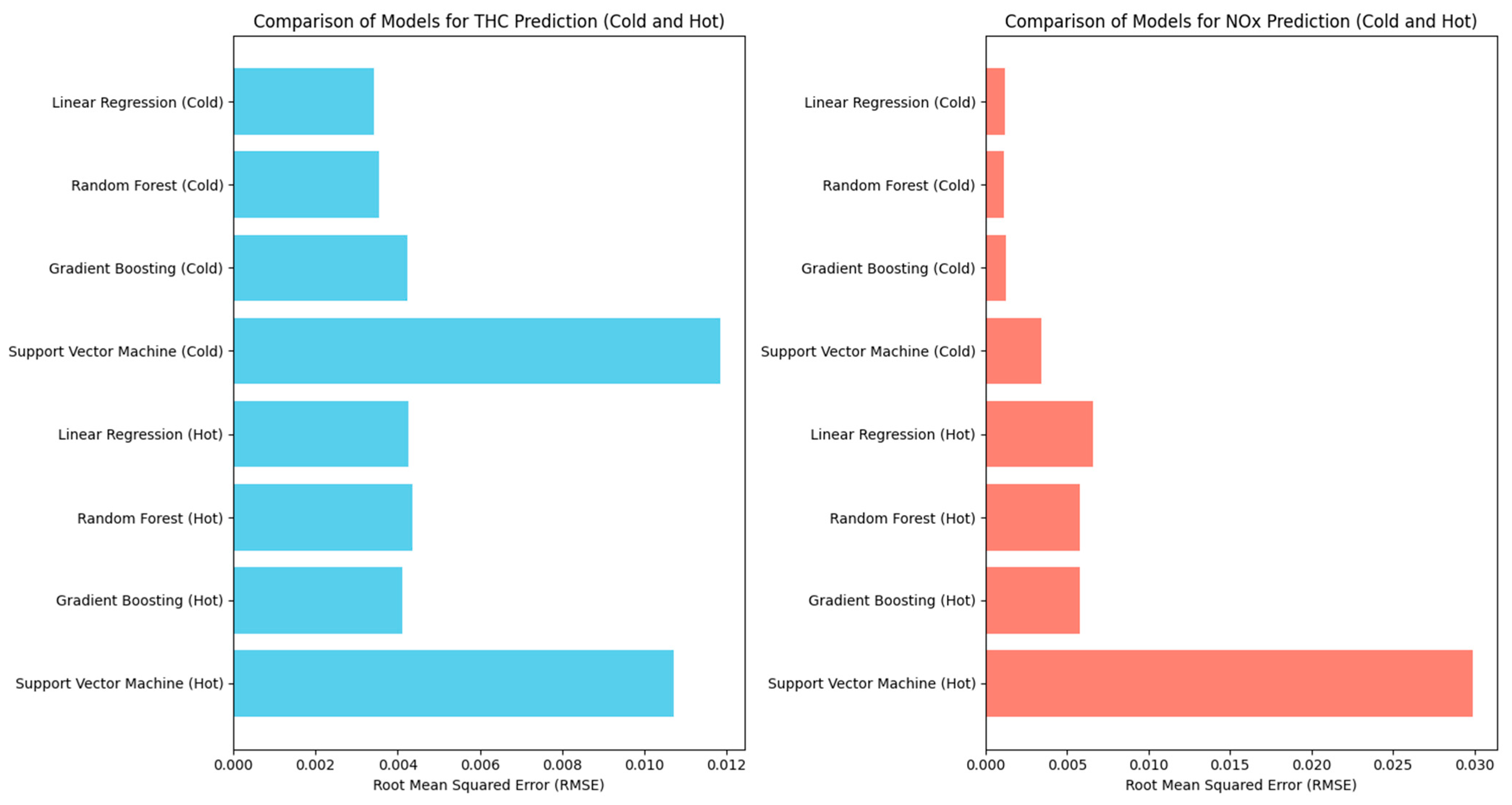
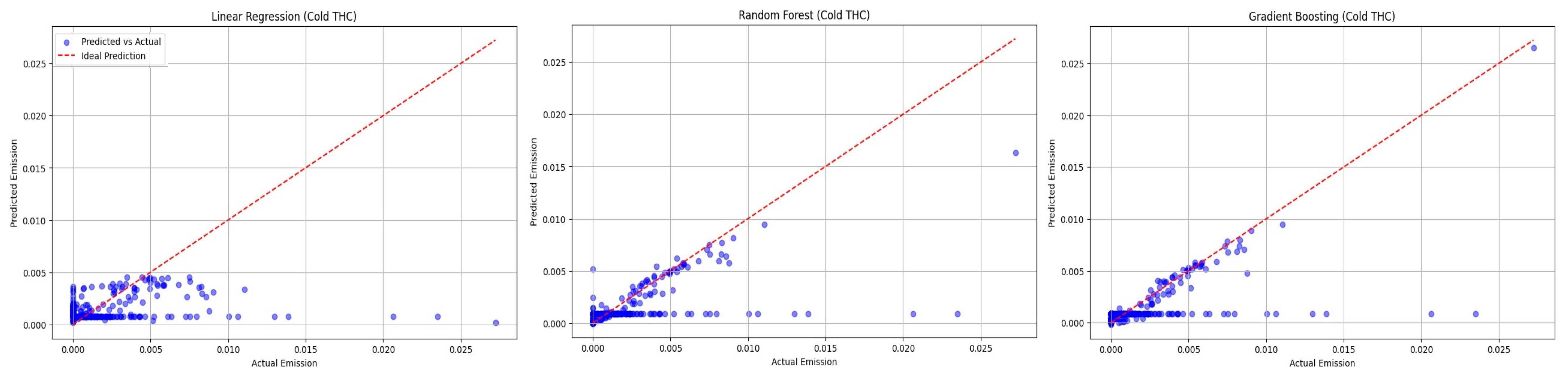
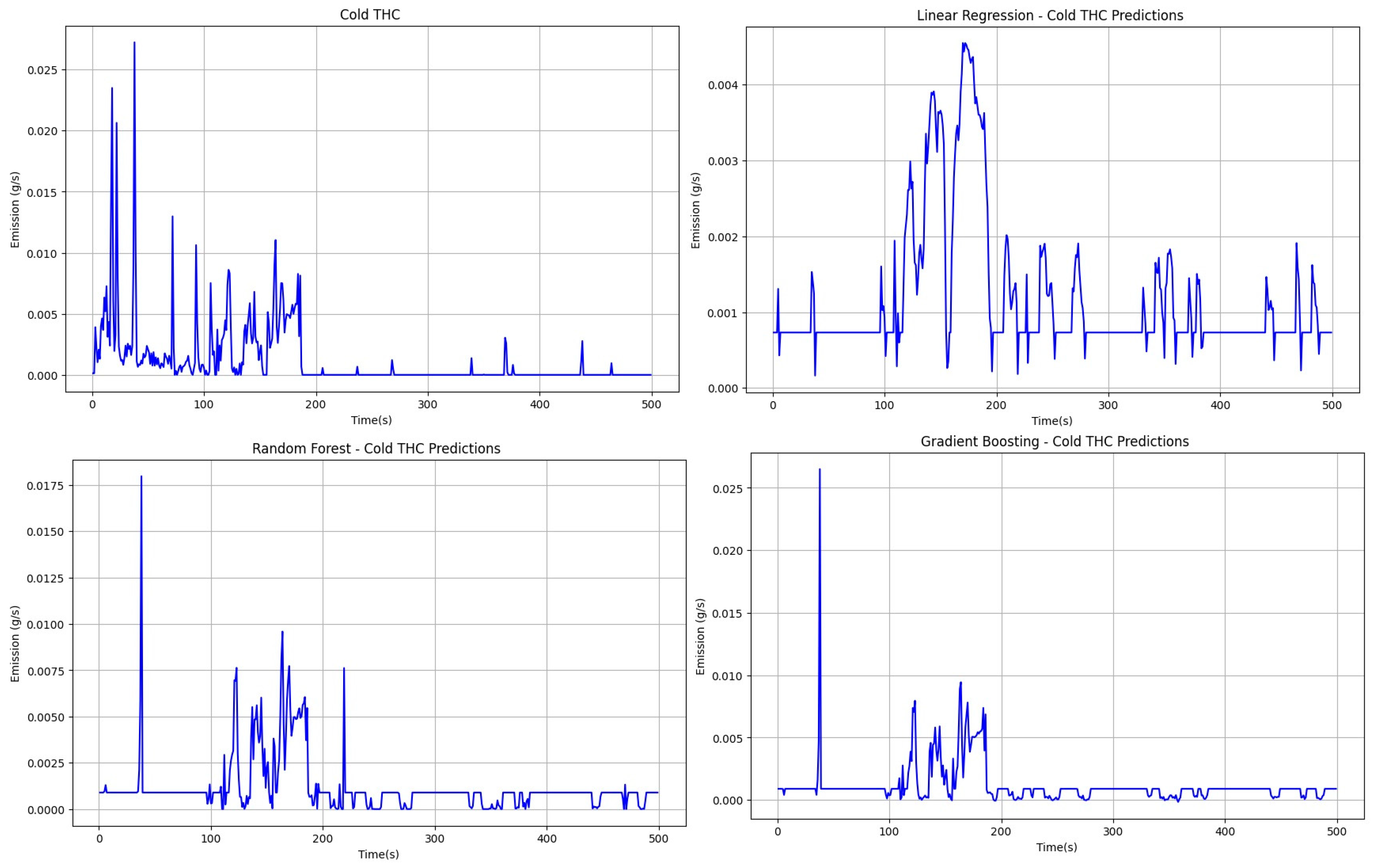
• Figure 11 compares the results of the curves plotted for the computational techniques examined for cold THC emissions. On the basis of this plot, it can be observed that the linear regression method exhibited the poorest predictive performance, while the random forest and gradient boosting methods showed comparable predictive capabilities for cold THC emissions.
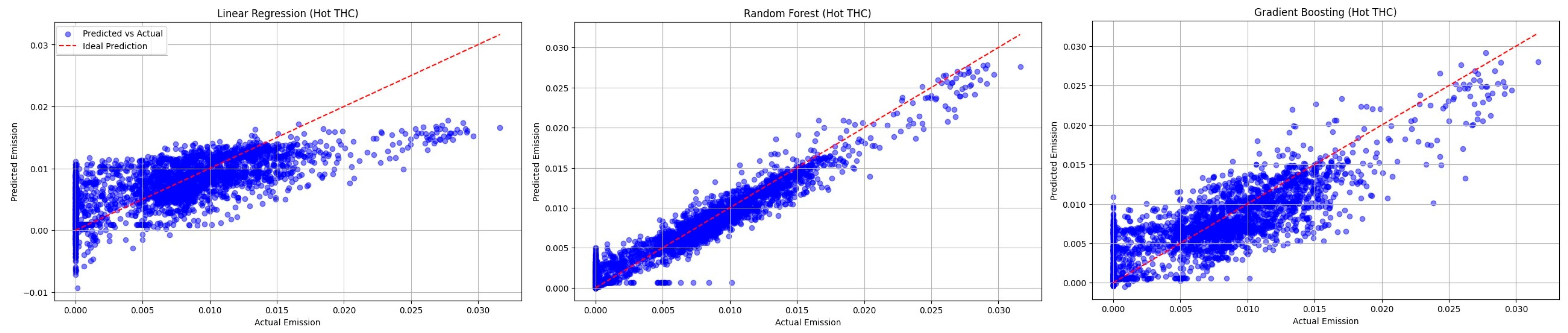
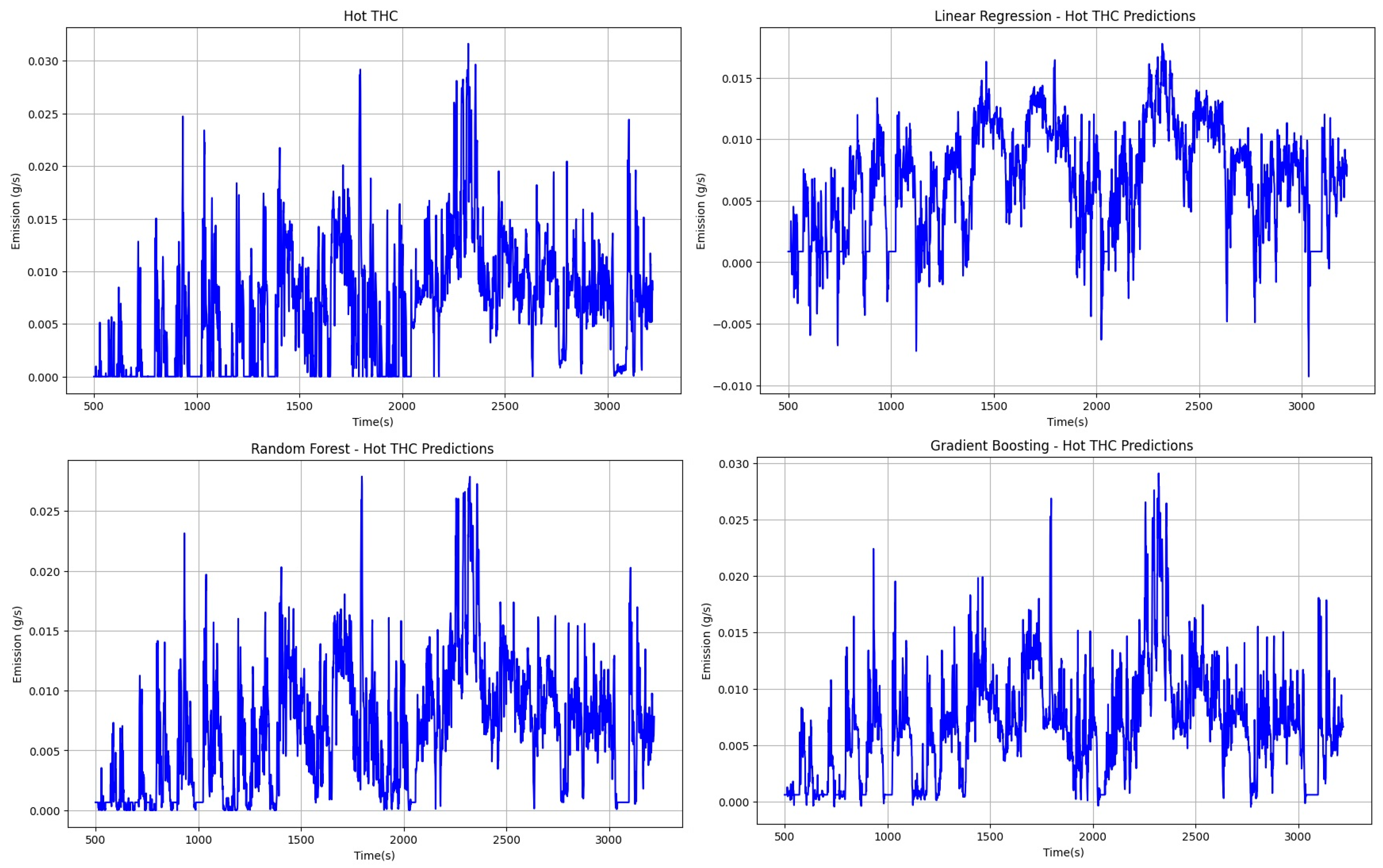
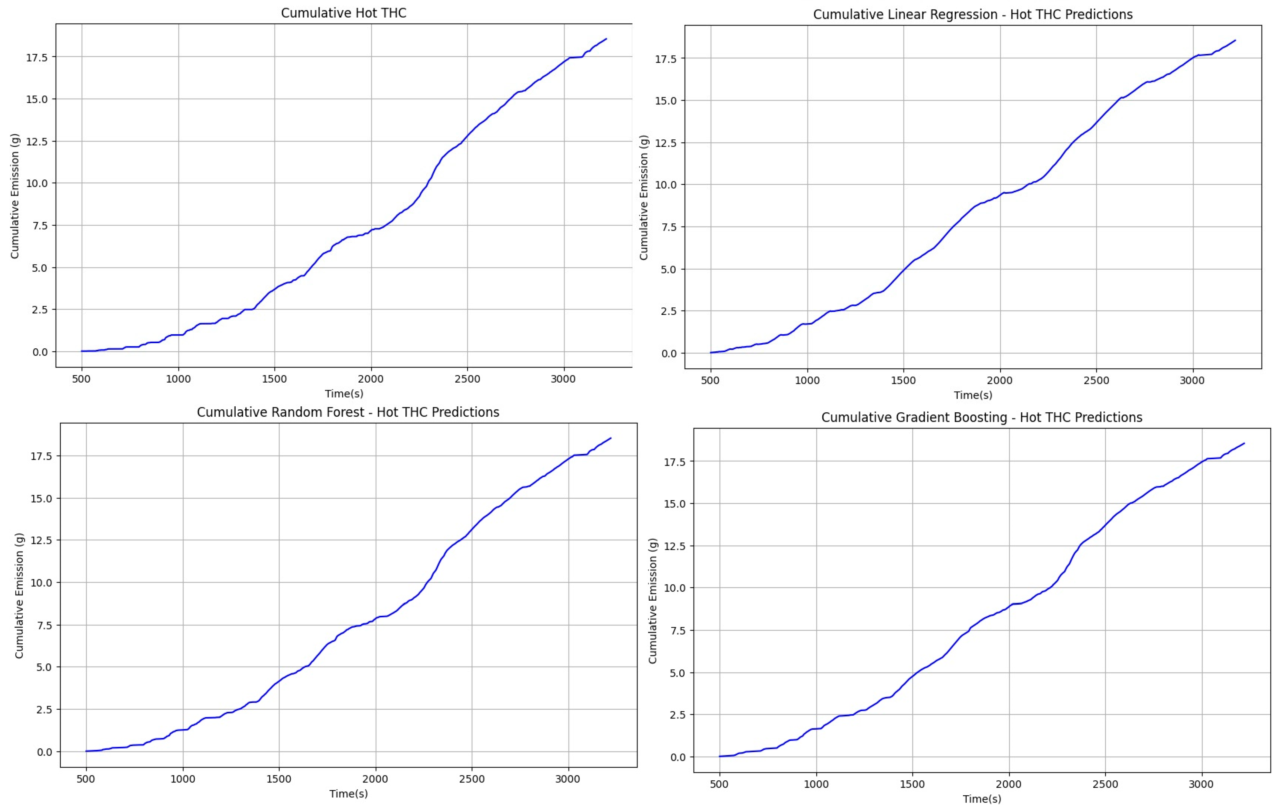
• Figure 12 illustrates the comparison of results for the techniques examined for hot THC emissions. Similarly to the previous plot, the linear regression method also demonstrated the poorest predictive abilities, as evidenced by the data points that deviated the most from the ideal line of data concordance marked in red. The random forest method provided the best reflection of the actual results compared to the model results, with the highest number of values close to the ideal curve.
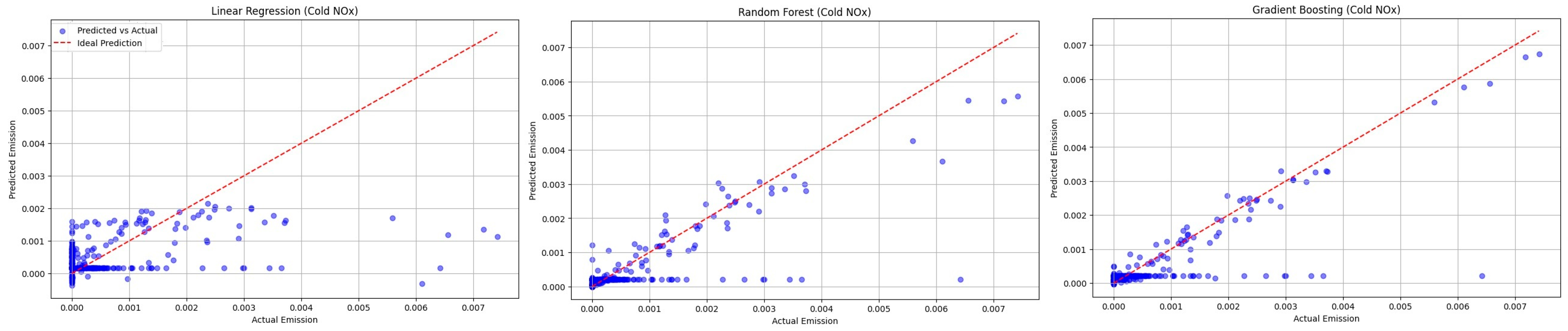
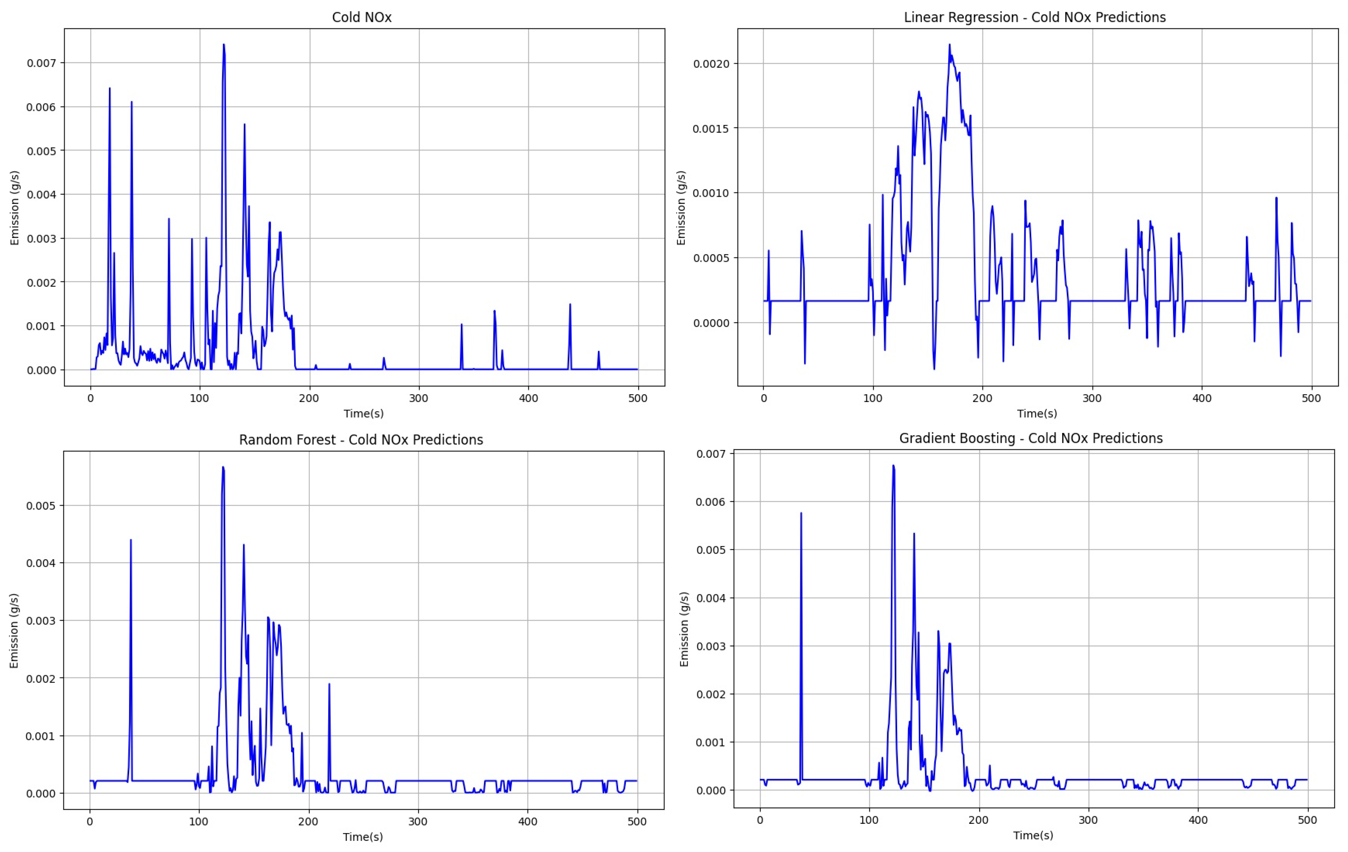
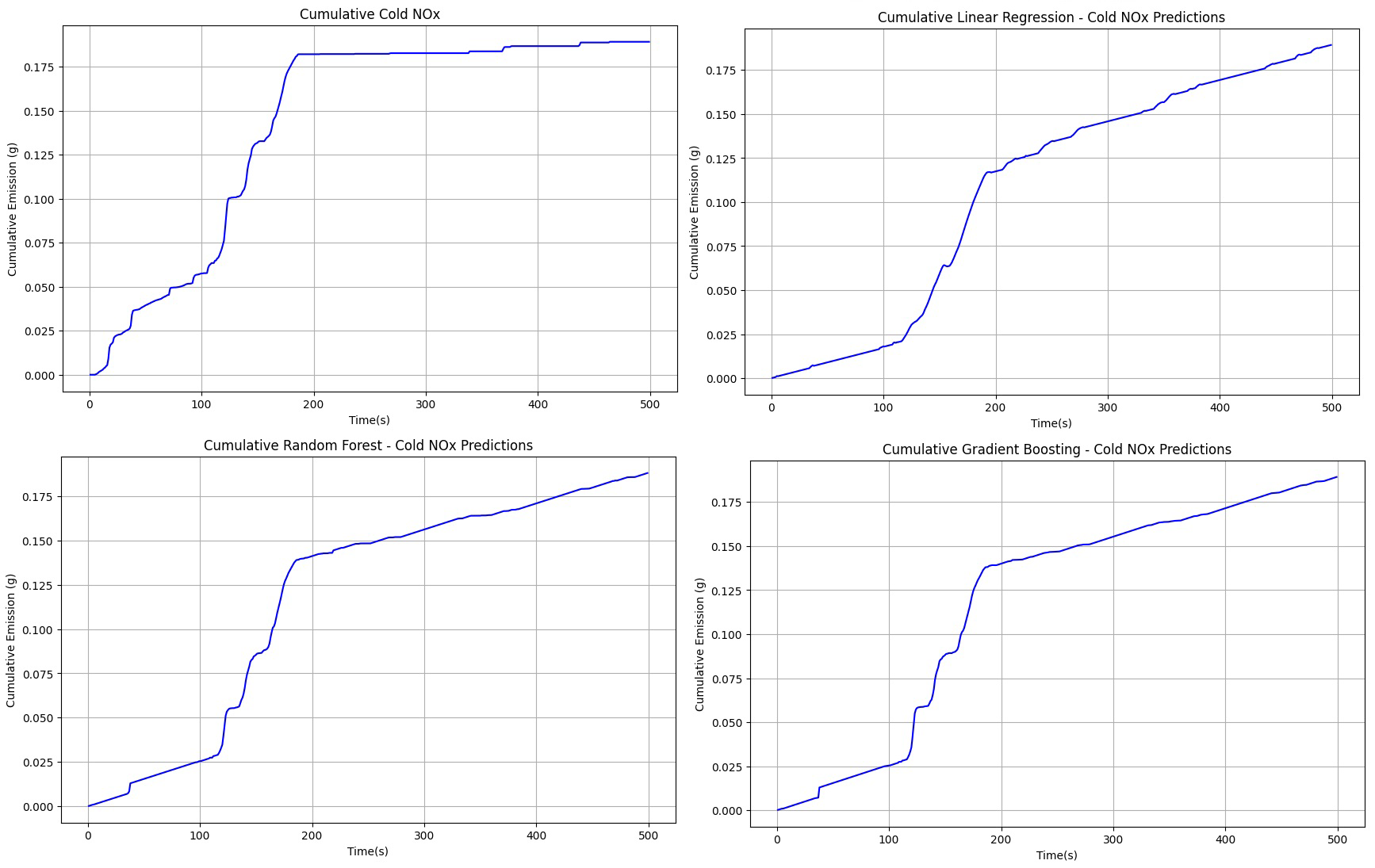
• For NOx emissions during a cold engine start, as shown in Figure 13, it can be observed that similar to THC emissions, random forest and gradient boosting techniques exhibited the best predictive abilities at a similar level, while the linear regression method produced the worst results.
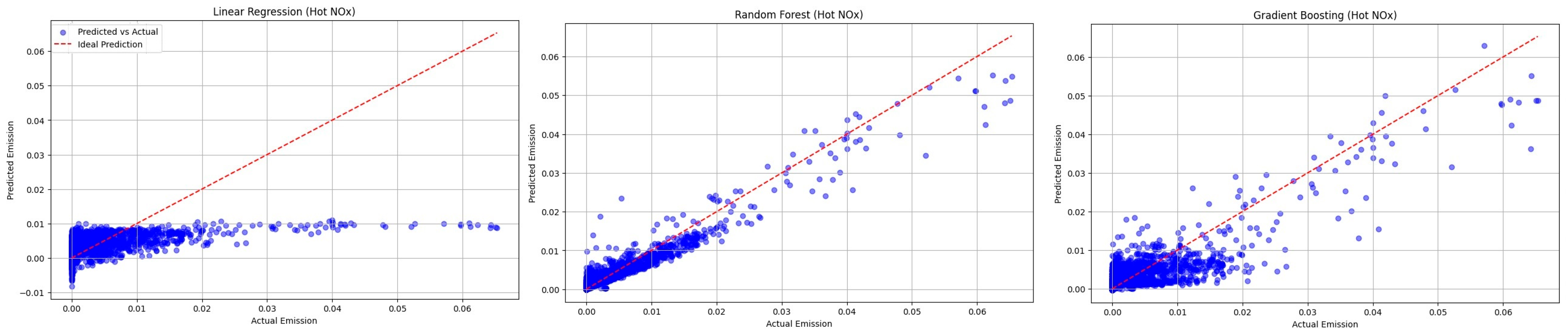
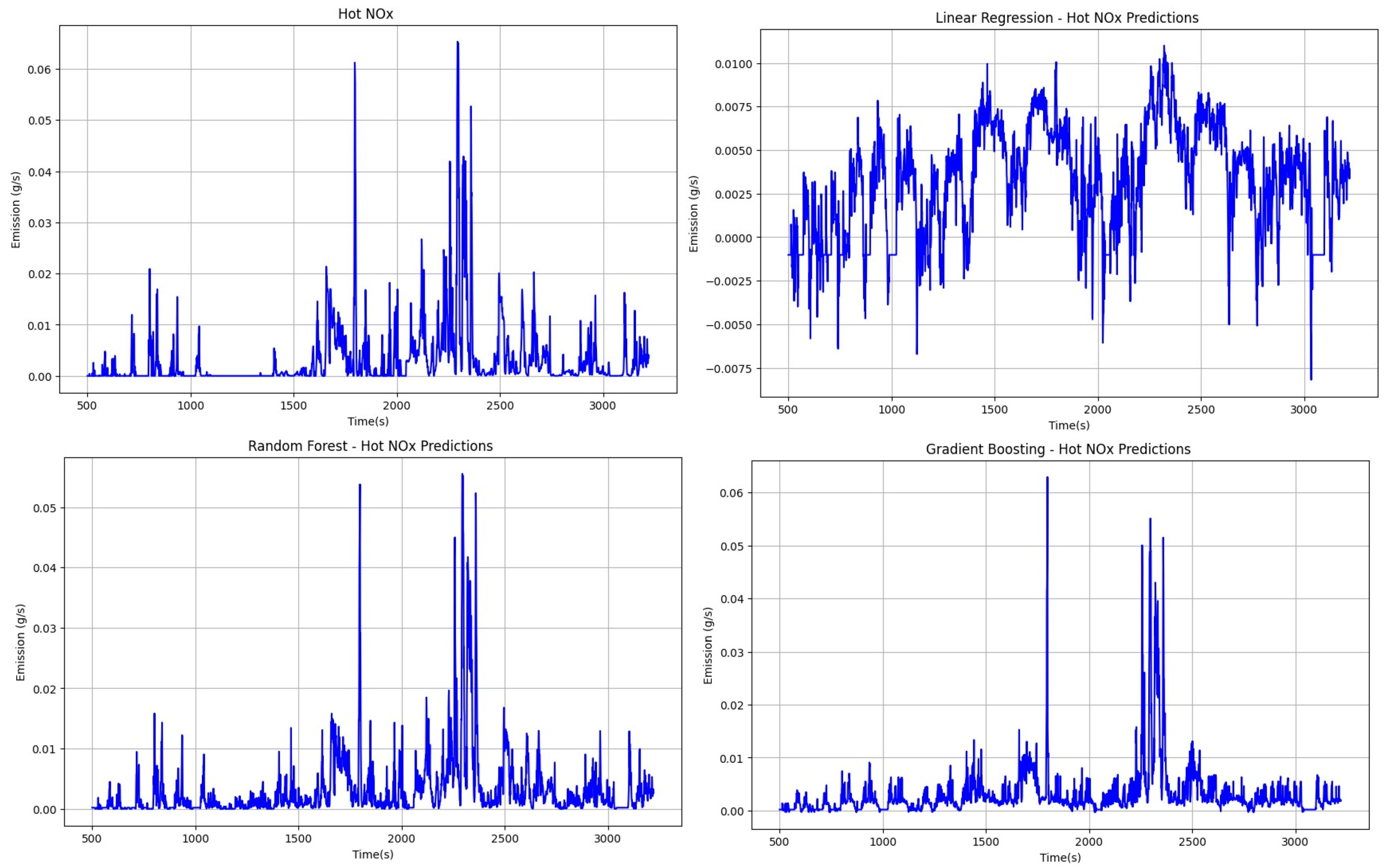
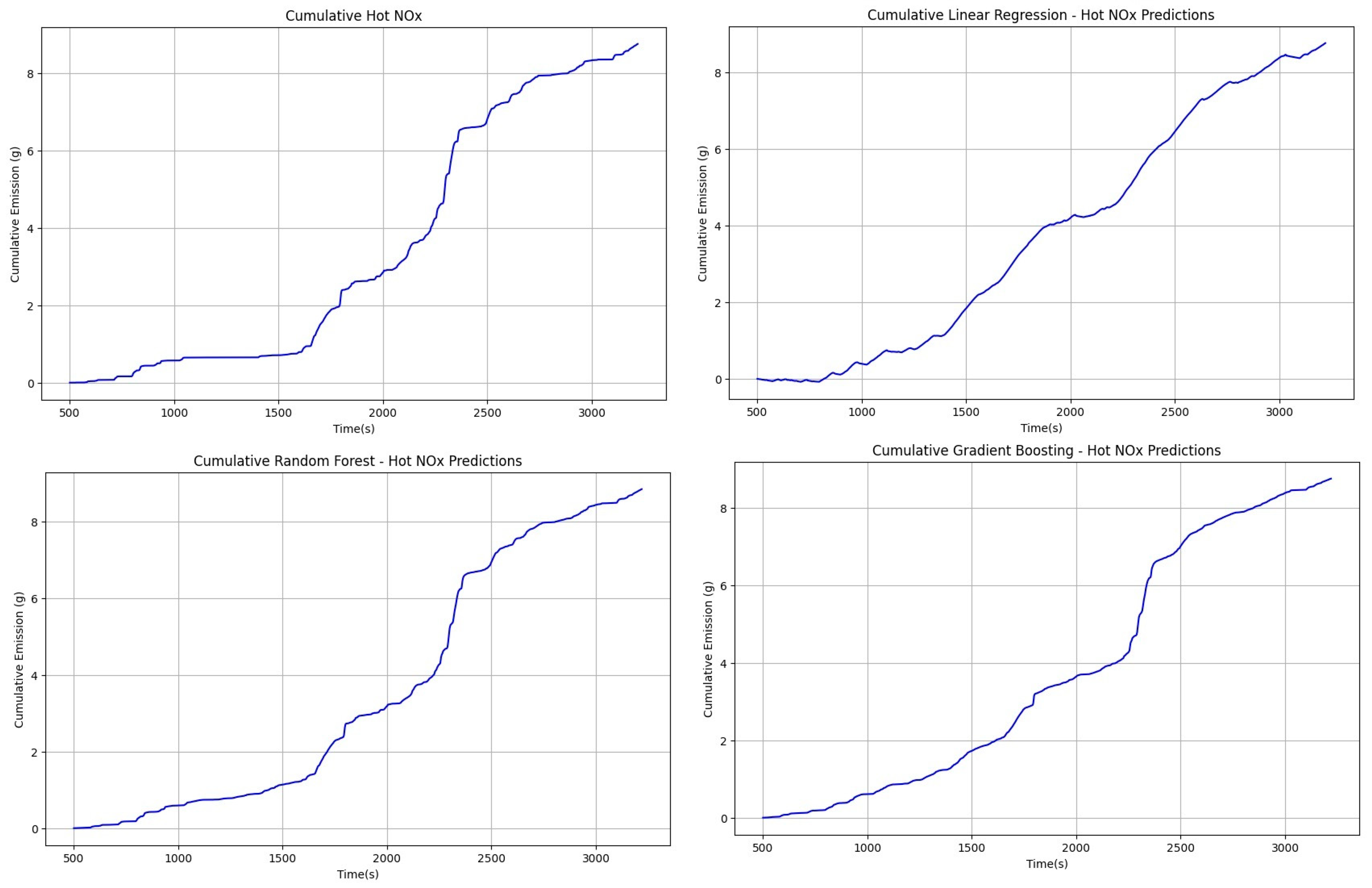
• For NOx emissions in a heated engine, the random forest method demonstrated the best predictive capabilities (Figure 14), while linear regression exhibited the weakest performance.

For the developed models of cold THC emissions, a comparison between predicted emissions and actual emissions was performed for a new set of data obtained from the road test, as shown in Figure 15.

For the data analyzed, comparative cumulative emission plots were also generated using different prediction methods. For cold THC emissions, this is presented in Figure 16.

The comparison of cumulative emissions in Figure 16 interestingly presents similar predictive capabilities of all models in estimating the total emission quantity. However, comparing these data with Figure 15, it can be observed that evaluating the models’ capabilities based on the sum of emissions can lead to incorrect conclusions.

The next validation step for the emission models obtained involved comparing the emissions obtained from a new road test with the emissions predicted by the models developed. Based on Figure 15, which presents a comparison of cold THC emissions, it can be observed that the emission model that performed the worst for the cold engine was the linear regression model. It showed a constant emission value with occasional spikes throughout the duration of the cold engine test. In the context of start–stop technology, it is crucial to obtain emission values close to zero, especially when the engine is idle. It is also worth noting that during the engine warm-up period, the start–stop system did not always activate, which can be observed in the first 200 s of the test. Models using random forest and gradient boost techniques demonstrated a slightly better reflection of actual emissions in this regard. It is important to emphasize that there was a weak correlation between the explanatory parameters “V” and “a” in relation to the emissions of the cold engine. This weak correlation makes it difficult to develop detailed emission models.

The next step involved the same validation process but for the emissions of a heated engine (Figure 17).

Based on Figure 17, it can be observed that for emissions from a heated engine in the THC range, predictive models yielded better results, especially for random forest and gradient boosting techniques. Unfortunately, the linear regression method led to an underestimation of results and additionally presented negative emission values. Moreover, this method could not reflect engine stop moments during the journey. The best predictive results were provided by the random forest method, which allowed for a very good reflection of transient THC emissions from the heated engine. The gradient boosting method performed slightly worse and, similar to linear regression, resulted in negative emission values.

Similar to cold THC emissions, a comparison of predictive capabilities was performed for hot THC emissions in terms of predictive performance (Figure 18).

In the analysis of Figure 18, similar conclusions can be drawn as in the case of analyzing the analogous plot for cold THC emissions. The total sum of emissions for all methods examined was very close.

After analyzing the predictive results for THC, the study presents a comparative analysis for NOx (Figures 19 and 21).

Based on Figure 19, which presents a comparison of emission results between actual values and predictive values, it can be observed that the linear regression method yielded the worst predictive capabilities, while the random forest and gradient boosting methods performed better. The linear regression method failed to capture vehicle stop moments, overestimated predictions and showed negative results. Random forest and gradient boosting methods exhibited similar predictive abilities, accurately reflecting NOx emissions within certain ranges. However, for cold engine emissions, these models do not yet provide satisfactory results for the designated explanatory variables.

The comparison of cumulative emissions for cold NOx for the predictive methods examined is presented in Figure 20.

Based on Figure 20, it can be observed that, similarly to previous cases, total cold NOx emissions were close for all scenarios analyzed here. However, in the range of 0–200 s, the methods of random forest and gradient boosting showed better capabilities in terms of the sum of emissions close to the actual emissions.

The final stage involved the validation of models for hot NOx emissions (Figure 21).

Based on Figure 21, which demonstrates the predictive capabilities of the developed models, it can be observed that the random forest and gradient boosting models closely reflected the actual emissions. The linear regression method led to negative emission estimates and completely failed to capture engine stop moments.

The comparison of cumulative hot NOx emissions is presented in Figure 22.

Analyzing Figure 22, it can be noticed that in terms of estimating the overall number of emissions, all the analyzed methods had similar predictive capabilities. However, when we considered detailed emission sums for the tested time period, for example, 1500–2500 s of the test, it can be observed that the random forest and gradient boosting methods exhibited significantly better capabilities in estimating cumulative emissions.

In the final stage of model verification, the models were compared based on the R-squared statistic. R-squared is a commonly used metric for assessing the quality of regression models. It expresses the degree to which the variability of dependent variables is explained by the model. The R² value ranges from 0 to 1, where a value closer to 1 indicates a better fit of the model to the data. The advantages of interpreting R² include its ease of understanding and the ability to compare different models. However, R² can be misleading for models with a large number of independent variables as it may indicate a high model fit even if there is a weak relationship between the variables [60]. Moreover, the R² value can be falsely high when using overly complex models, limiting its usefulness as the only indicator of model evaluation. Therefore, it is important to consider R² in model evaluations but with caution and in conjunction with other evaluation metrics.

The results of the R² statistic for the models obtained are presented in

Table 2. Results of the R² for the predictive methods analyzed.

Method/Result	R2 (THC)	R2 (NOx)
Linear regression (Cold)	0.25	0.21
Random forest (Cold)	0.3	0.28
Gradient boosting (Cold)	0.33	0.3
Linear regression (Hot)	0.42	0.35
Random forest (Hot)	0.91	0.92
Gradient boosting (Hot)	0.88	0.85

.

Based on Table 2, it can be observed that, generally, the emission models for both THC and NOx during a cold start exhibited a relatively low predictive ability. This is associated with limitations in the explanatory variables for the model, as described earlier. On the basis of previous analyses, especially for random forest and gradient boosting models, they may provide some predictive capability, especially for moments of emission spikes to high values. Regarding the emissions for the heated engine, very good predictive capabilities can be observed in terms of the R² statistic for random forest and gradient boosting methods. This is further confirmed by earlier graphical analyses of predicted vs. actual plots and predicted emission plots.

The validation of the obtained models was multistage and included the analysis of R² and RMSE indicators. However, considering the limitations of interpreting models based on these metrics, their validation was expanded to include an analysis of predicted vs. actual emission plots and prediction results of THC and NOx emissions for new datasets. Therefore, in the discussion section below, recommendations are described on the issue of modeling emissions from vehicles equipped with start–stop technology.

4. Discussion

The developed research methodology allows for a detailed examination of the process of creating THC and NOx emission models for vehicles equipped with start–stop technology. The added value of such models is their ability to predict potential engine stop locations where no emissions occur, compared to commonly available models on a microscale. The utility of these models can be significant as they allow for estimating transient emissions for analyzed road segments, average emissions, and cumulative emissions. Such capabilities are necessary for transportation decision makers and professionals involved in, among other things, vehicle traffic modeling. Environmental analyses in these aspects are an integral part of designing future road solutions and validating existing ones.

It is also worth mentioning that this is one of the first works focusing on modeling emissions from vehicles equipped with start–stop technology. It is the first study to specifically address the modeling of NOx and THC emissions from such vehicles. The only similar work is [61]. This article presents a novel methodology to measure and model CO₂ emissions in vehicles equipped with start–stop technology. Using artificial intelligence techniques, the method accurately predicts CO₂ emissions using only velocity, acceleration, and road gradient data. Three machine learning techniques were evaluated, with gradient boosting demonstrating the best prediction performance. The validation of the developed models was carried out using the coefficient of determination, the mean squared error, and visual assessment of the residual plots and CO₂ emission maps. These models offer a promising approach to microscale environmental analysis. Another similar study utilizing artificial intelligence methods for modeling is [62]. This study responds to the pressing demand for precise prediction models of CO₂ emissions from vehicles powered by compressed natural gas (CNG), given the escalating stringency of global environmental policies. By combining experimentation and modeling, this research develops a CO₂ emission model specifically for CNG-powered vehicles. The study leverages data from both chassis dynamometer tests and road assessments using a Portable Emission Measurement System (PEMS) and implements the XGBoost algorithm within the Optuna Python programming framework. Another study that also applies machine learning techniques and focuses on modeling NOx emissions from diesel engines is [63]. This study applies machine learning techniques to develop accurate instantaneous vehicle emissions models, which are crucial for assessing the impact of road transport on air pollution with high temporal and spatial resolution. By analyzing a dataset of 70 diesel vehicles tested in real-world driving conditions, the study successfully clusters vehicles with similar emissions performance and models instantaneous emissions. Using dynamic time warping and clustering analysis, NOx emission data were grouped into 17 clusters, covering 88% of the trips in the dataset. Despite the lack of a significant correlation between emissions and vehicle characteristics, such as engine size or vehicle weight, the clustering successfully grouped vehicles with similar emission profiles. For each cluster, three models were assessed: a neural network multilayer perceptron (MLP) model, a nonlinear regression (NLR) model, and a look-up table (LT) approach. Artificial intelligence methods have been applied to model the energy usage of electric vehicles [64,65,66]. This particular study [64] outlines the methodology used to develop a model for electric vehicle (EV) energy consumption, allowing for rapid result generation and the creation of energy maps. Among the validation techniques employed, artificial intelligence, specifically neural networks, demonstrated the most robust performance. Within this framework, two predictive models for EV energy consumption were constructed, tailored to winter and summer conditions and based on real driving patterns, offering significant implications for microscale road analyses. The resulting model, validated with summer test data, achieved an R² of 86% and an MSE of 1.4. Similarly, under winter conditions, the model reached values of 89% and 2.8, respectively, indicating its high precision.

There are also a number of studies that, unlike the regression models mentioned above, use classification methods and data processing to estimate vehicle emissions. One such study is [67]. This article introduces a methodology for estimating emissions in real driving conditions using onboard diagnostic data and machine learning, addressing the absence of models for pollutant estimation without extensive measurement campaigns. Driving data are collected using a data logger, and emissions are measured using a portable emissions measurement system during real driving emissions tests. Artificial neural networks are trained using these data to estimate emissions, with the importance of variables being assessed beforehand using random forest techniques. The K-means algorithm is then applied to obtain labels for implementing a classification tree to determine the gear selected by the driver. These models were trained using a dataset that covers 1218.19 km of driving.

There is also a growing popularity in emission modeling using strictly artificial neural network models. An example of such a study can be found in [68]. This article introduces a novel approach to predict carbon dioxide (CO₂), nitrogen oxides (NOx), and carbon monoxide (CO) emissions from diesel vehicles using artificial neural networks (ANNs), known for their precision and practicality. Six operating parameters obtained through the onboard diagnostic interface were utilized as predictors of exhaust emissions. The importance of each parameter in emission predictions was thoroughly analyzed through various metrics, such as the coefficient of determination, root mean square error, cumulative emissions, and instantaneous emission rates. The accuracy of emission prediction by ANNs tends to improve as more parameters are included as model inputs, albeit with varying levels of improvement depending on the parameters. In particular, engine torque and fuel/air ratio emerged as significant predictors of CO₂ emissions, while the intake air mass flow rate and fuel/air ratio were crucial for NOx and CO predictions, respectively. However, it is worth considering the practicality of such models, as the predictors used for emission estimation may be impractical and difficult to collect during regular road trips.

In the literature related to the developed topic, there has been an increasing popularity of such studies in the last 5 years. There are various methods that range from simple estimations to advanced techniques using neural networks. However, so far, little attention has been paid to the aspect of emission modeling for vehicles equipped with start–stop systems, so this work is a response to this research gap. As part of the studies conducted, a set of main conclusions and recommendations have been prepared regarding the problem of emission modeling for vehicles equipped with start–stop systems, which are presented below.

Recommendations for Modeling THC and NOx Emissions for a Vehicle Equipped with Start–Stop Technology

Through the course of conducting this study and analyzing the obtained results, several recommendations for further development of such emission models emerge:

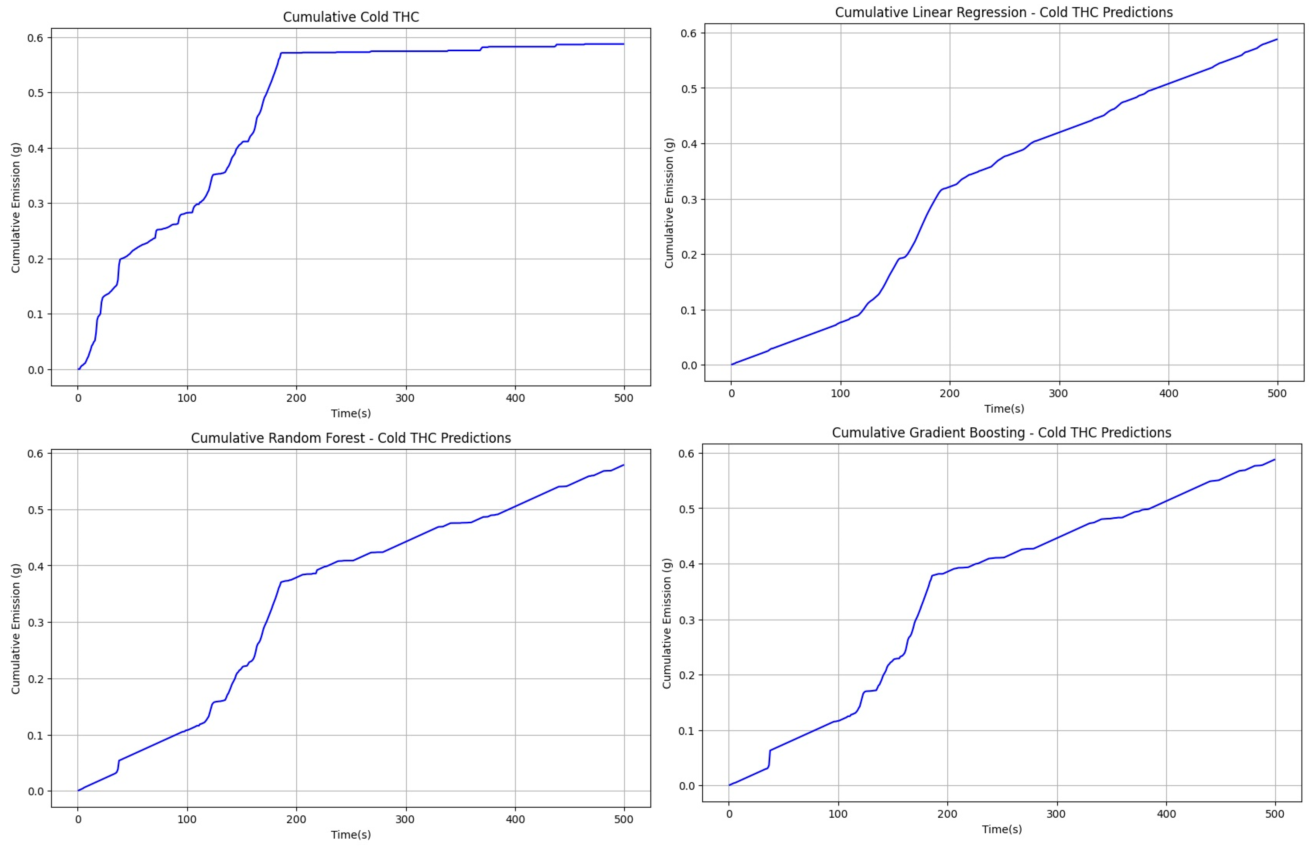
• Crucial for modeling such emissions are the predictive capabilities for moments when the engine is stopped and no emissions occur. Therefore, the search for predictive methods should begin with evaluating their ability to predict the vehicle’s idle periods.
• Random forest and gradient boosting techniques provide rapid results and demonstrate the best predictive abilities for both cold and hot emissions from vehicles equipped with start–stop technology.
• Unfortunately, the linear regression method leads to a significant underestimation of emission generation results. Additionally, the generation of negative emission results from this model disqualifies its potential use in modeling emissions from such vehicles.
• Validation of the obtained THC and NOx emission models for start–stop vehicles must be multistage. Therefore, only relying on performance indicators such as R² and RMSE is insufficient. It is best to supplement these with predicted vs. actual plots, which can, for example, reveal if a particular method predicts negative emission values.

5. Conclusions

The paper presents the process of creating models of THC and NOx emissions for vehicles equipped with start–stop technology. On the basis of the developed results, the main conclusions drawn from the study are as follows:

• The linear regression technique exhibited the worst predictive capabilities, both for emissions from cold and hot engines. It led to underestimation and negative emission values in certain driving ranges. For example, the R² values for cold THC emissions were 0.25, and for NOx emissions, they were 0.21.
• For the models developed for cold THC and NOx emissions, other computationally more advanced methods, such as random forest and gradient boosting, also exhibited weak predictive capabilities. Respectively, for these methods, the R² values were 0.3 and 0.33 for THC emissions and 0.28 and 0.3 for NOx emissions. This was related to the analysis of the correlation between the explanatory input variables of the model and the emission variable.
• Random forest and gradient-boosting techniques demonstrated very good predictive capabilities for emissions from a heated engine. Specifically, for these methods, the R² values for THC emissions were 0.91 and 0.88, and for NOx emissions, they were 0.92 and 0.85. The accuracy of the developed models was also reflected in the validation plots of predicted vs. actual values and predictions in a new dataset.

The methodologies developed to create THC and NOx emission models can be scalable to other harmful exhaust components and vehicles. In this context, there is also potential for the utilization of such models for hybrid vehicles as they also do not emit harmful exhaust components when switching to electric mode. In this aspect, the predictive abilities for the moments of switching off the combustion engine will be crucial, which is presented in this work using the example of the start–stop system. Therefore, this work contributes to understanding the potential of computational techniques for developing similar exhaust emission models. Future directions of work certainly involve expanding the developed models to include additional input datasets, testing additional vehicles, and considering the use of other artificial intelligence computational techniques to obtain rapid emission results.

It is worth noting that the goal of the work was to create emission models that were as universal as possible. That is why such a choice of input data for model training was made. Of course, this has limitations in the form of limited predictive abilities for the cold start model. This work is an example of how vehicle motion data such as speed and acceleration provide good predictive abilities for estimations within certain driving ranges but not necessarily in the areas of cold emission modeling. This does not mean, however, that such models will not accurately estimate the average emission rate or total emissions for such engine operating conditions.

References

1. Zhang, L.; Weng, D.; Xu, Y.; Hong, B.; Wang, S.; Hu, X.; Zhang, Y.; Wang, Z. Spatio-temporal evolution characteristics of carbon emissions from road transportation in the mainland of China from 2006 to 2021. Sci. Total Environ. 2024, 917, 170430. [Google Scholar] [CrossRef] [PubMed]
2. Albuquerque, F.D.; Maraqa, M.A.; Chowdhury, R.; Mauga, T.; Alzard, M. Greenhouse gas emissions associated with road transport projects: Current status, benchmarking, and assessment tools. Transp. Res. Procedia 2020, 48, 2018–2030. [Google Scholar] [CrossRef]
3. Duan, L.; Hu, W.; Deng, D.; Fang, W.; Xiong, M.; Lu, P.; Li, Z.; Zhai, C. Impacts of reducing air pollutants and CO2 emissions in urban road transport through 2035 in Chongqing, China. Environ. Sci. Ecotechnol. 2021, 8, 100125. [Google Scholar] [CrossRef] [PubMed]
4. Cunanan, C.; Tran, M.K.; Lee, Y.; Kwok, S.; Leung, V.; Fowler, M. A review of heavy-duty vehicle powertrain technologies: Diesel engine vehicles, battery electric vehicles, and hydrogen fuel cell electric vehicles. Clean Technol. 2021, 3, 474–489. [Google Scholar] [CrossRef]
5. Bai, S.; Liu, C. Overview of energy harvesting and emission reduction technologies in hybrid electric vehicles. Renew. Sustain. Energy Rev. 2021, 147, 111188. [Google Scholar] [CrossRef]
6. Kuszewski, H.; Jaworski, A.; Mądziel, M. Lubricity of Ethanol–Diesel Fuel Blends—Study with the Four-Ball Machine Method. Materials 2021, 14, 2492. [Google Scholar] [CrossRef] [PubMed]
7. Kuszewski, H.; Jaworski, A.; Mądziel, M.; Woś, P. The investigation of auto-ignition properties of 1-butanol–biodiesel blends under various temperatures conditions. Fuel 2023, 346, 128388. [Google Scholar] [CrossRef]
8. Yu, X.; Sandhu, N.S.; Yang, Z.; Zheng, M. Suitability of energy sources for automotive application–A review. Appl. Energy 2020, 271, 115169. [Google Scholar] [CrossRef]
9. Alkawsi, G.; Baashar, Y.; Abbas, U.D.; Alkahtani, A.A.; Tiong, S.K. Review of renewable energy-based charging infrastructure for electric vehicles. Appl. Sci. 2021, 11, 3847. [Google Scholar] [CrossRef]
10. Madichetty, S.; Mishra, S.; Basu, M. New trends in electric motors and selection for electric vehicle propulsion systems. IET Electr. Syst. Transp. 2021, 11, 186–199. [Google Scholar] [CrossRef]
11. De Paulo, A.F.; Nunes, B.; Porto, G. Emerging green technologies for vehicle propulsion systems. Technol. Forecast. Soc. Change 2020, 159, 120054. [Google Scholar] [CrossRef]
12. Wang, D.; Jiang, M.; He, K.; Li, X.; Li, F. Study on vibration suppression method of vehicle with engine start-stop and automatic start-stop. Mech. Syst. Signal Process. 2020, 142, 106783. [Google Scholar] [CrossRef]
13. Zhu, R.; Fu, Y.; Wang, L.; Hu, J.; He, L.; Wang, M.; Lai, Y.; Su, S. Effects of a start-stop system for gasoline direct injection vehicles on fuel consumption and particulate emissions in hot and cold environments. Environ. Pollut. 2022, 308, 119689. [Google Scholar] [CrossRef] [PubMed]
14. Santos, N.D.S.A.; Roso, V.R.; Faria, M.T.C. Review of engine journal bearing tribology in start-stop applications. Eng. Fail. Anal. 2020, 108, 104344. [Google Scholar] [CrossRef]
15. Chen, B.; Pan, X.; Evangelou, S.A. Optimal Energy Management of Series Hybrid Electric Vehicles with Engine Start–Stop System. IEEE Trans. Control Syst. Technol. 2022, 31, 660–675. [Google Scholar] [CrossRef]
16. Barbashov, N.; Polyantseva, A. Method of electric vehicle braking energy recovery. E3S Web Conf. 2024, 471, 02010. [Google Scholar] [CrossRef]
17. Briguiet, G.D.O.F.; Lopes, P.H.L.M.; Rodrigues, G.S.; Lopes, E.D.R. Investigation of Powertrains in Hybrid Vehicles (No. 2020-36-0137); SAE Technical Paper; SAE: Warrendale, PA, USA, 2021. [Google Scholar]
18. He, L.; You, Y.; Zheng, X.; Zhang, S.; Li, Z.; Zhang, Z.; Wu, Y.; Hao, J. The impacts from cold start and road grade on real-world emissions and fuel consumption of gasoline, diesel and hybrid-electric light-duty passenger vehicles. Sci. Total Environ. 2022, 851, 158045. [Google Scholar] [CrossRef]
19. Yang, Z.; Xu, H.; Yu, H.; Liu, Y.; Xing, J. Analysis of Emissions Characteristics and Fuel Consumption of Light-Duty Passenger Vehicles under Different Driving Cycles. In Proceedings of the 2023 4th International Conference on Clean and Green Energy Engineering (CGEE), Ankara, Turkey, 26–28 August 2023; pp. 106–111. [Google Scholar]
20. Da Silva, S.F.; Eckert, J.J.; Silva, F.L.; e Silva, L.C.D.A.; Dedini, F.G. Modeling and Simulation of Start/Stop System for Reduction of Vehicle Fuel Consumption and Air Pollutant Emissions; Brazilian Society of Automotive Engineering: São Paulo, Brazil, 2021. [Google Scholar]
21. Mera, Z.; Fonseca, N.; Casanova, J.; López, J.M. Influence of exhaust gas temperature and air-fuel ratio on NOx aftertreatment performance of five large passenger cars. Atmos. Environ. 2021, 244, 117878. [Google Scholar] [CrossRef]
22. Zhang, H.W.; Tsai, Z.R.; Kok, V.C.; Peng, H.C.; Chen, Y.H.; Tsai, J.J.; Hsu, C.Y. Long-term ambient hydrocarbon exposure and incidence of urinary bladder cancer. Sci. Rep. 2022, 12, 20799. [Google Scholar] [CrossRef] [PubMed]
23. Zhao, M.; Xue, P.; Liu, J.; Liao, J.; Guo, J. A review of removing SO2 and NOX by wet scrubbing. Sustain. Energy Technol. Assess. 2021, 47, 101451. [Google Scholar] [CrossRef]
24. Khani, M.R.; Barzideh Pour, E.; Rashnoo, S.; Tu, X.; Ghobadian, B.; Shokri, B.; Khadem, A.; Hosseini, S.I. Real diesel engine exhaust emission control: Indirect non-thermal plasma and comparison to direct plasma for NO x, THC, CO, and CO 2. J. Environ. Health Sci. Eng. 2020, 18, 743–754. [Google Scholar] [CrossRef] [PubMed]
25. Ndletyana, O.; Madonsela, B.S.; Maphanga, T. Spatial Distribution of PM 10 and NO 2 in Ambient Air Quality in Cape Town CBD, South Africa. Nat. Environ. Pollut. Technol. 2023, 22, 1–13. [Google Scholar] [CrossRef]
26. Kulshrestha, U. Acid rain. In Managing Air Quality and Energy Systems; CRC Press: Boca Raton, FL, USA, 2020; pp. 707–727. [Google Scholar]
27. Zhang, L. Effects of Acid Rain on Forest Organisms and Countermeasures. Highlights Sci. Eng. Technol. 2023, 69, 292–298. [Google Scholar] [CrossRef]
28. Ihedike, C.; Ling, J. Effects of Ozone, Particulate Matter10 and Oxides of Nitrogen on Respiratory Health (COPD and asthma) in Nigeria: A Systematic Review. Lupine Online J. Nurs. Health Care 2022, 3, 364–371. [Google Scholar]
29. Kotyla, M.; Banasiewicz, A.; Krot, P.; Śliwiński, P.; Zimroz, R. NOx Emission Prediction of Diesel Vehicles in Deep Underground Mines Using Ensemble Methods. Electronics 2024, 13, 1095. [Google Scholar] [CrossRef]
30. Mądziel, M.; Campisi, T. Investigation of Vehicular Pollutant Emissions at 4-Arm Intersections for the Improvement of Integrated Actions in the Sustainable Urban Mobility Plans (SUMPs). Sustainability 2023, 15, 1860. [Google Scholar] [CrossRef]
31. Karami, Z.; Kashef, R. Smart transportation planning: Data, models, and algorithms. Transp. Eng. 2020, 2, 100013. [Google Scholar] [CrossRef]
32. Zhou, L.; Dang, X.; Sun, Q.; Wang, S. Multi-scenario simulation of urban land change in Shanghai by random forest and CA-Markov model. Sustain. Cities Soc. 2020, 55, 102045. [Google Scholar] [CrossRef]
33. Yang, H.; Almutairi, F.; Rakha, H. Eco-driving at signalized intersections: A multiple signal optimization approach. IEEE Trans. Intell. Transp. Syst. 2020, 22, 2943–2955. [Google Scholar] [CrossRef]
34. Tumminello, M.L.; Macioszek, E.; Granà, A.; Giuffrè, T. A Methodological Framework to Assess Road Infrastructure Safety and Performance Efficiency in the Transition toward Cooperative Driving. Sustainability 2023, 15, 9345. [Google Scholar] [CrossRef]
35. Fang, X.; Tettamanti, T. Change in microscopic traffic simulation practice with respect to the emerging automated driving technology. Period. Polytech. Civ. Eng. 2022, 66, 86–95. [Google Scholar] [CrossRef]
36. Severino, A.; Pappalardo, G.; Olayode, I.O.; Canale, A.; Campisi, T. Evaluation of the environmental impacts of bus rapid transit system on turbo roundabout. Transp. Eng. 2022, 9, 100130. [Google Scholar] [CrossRef]
37. Mądziel, M. Vehicle Emission Models and Traffic Simulators: A Review. Energies 2023, 16, 3941. [Google Scholar] [CrossRef]
38. Massaguer, A.; Pujol, T.; Comamala, M.; Massaguer, E. Feasibility study on a vehicular thermoelectric generator coupled to an exhaust gas heater to improve aftertreatment’s efficiency in cold-starts. Appl. Therm. Eng. 2020, 167, 114702. [Google Scholar] [CrossRef]
39. Liu, C.; Pei, Y.; Wu, C.; Zhang, F.; Qin, J. Novel insights into the NOx emissions characteristics in PEMS tests of a heavy-duty vehicle under different payloads. J. Environ. Manag. 2023, 348, 119400. [Google Scholar] [CrossRef] [PubMed]
40. Yang, Z.; Liu, Y.; Wu, L.; Martinet, S.; Zhang, Y.; Andre, M.; Mao, H. Real-world gaseous emission characteristics of Euro 6b light-duty gasoline-and diesel-fueled vehicles. Transp. Res. Part D Transp. Environ. 2020, 78, 102215. [Google Scholar] [CrossRef]
41. Zimakowska-Laskowska, M.; Laskowski, P.; Zasina, D. The Impact of the Fleet Age Structure on the Cold-Start Emission. Case Study of the Polish Passenger C and Light Commercial Vehicles (No. 2020-01-2091); SAE Technical Paper; SAE: Warrendale, PA, USA, 2020. [Google Scholar]
42. Mądziel, M. Liquified Petroleum Gas-Fuelled Vehicle CO2 Emission Modelling Based on Portable Emission Measurement System, On-Board Diagnostics Data, and Gradient-Boosting Machine Learning. Energies 2023, 16, 2754. [Google Scholar] [CrossRef]
43. Seo, J.; Yun, B.; Kim, J.; Shin, M.; Park, S. Development of a cold-start emission model for diesel vehicles using an artificial neural network trained with real-world driving data. Sci. Total Environ. 2022, 806, 151347. [Google Scholar] [CrossRef]
44. Smit, R.; Ntziachristos, L. Cold start emission modelling for the Australian petrol fleet. Air Qual. Clim. Change 2013, 47, 31–39. [Google Scholar]
45. Ziółkowski, A.; Fuć, P.; Lijewski, P.; Bednarek, M.; Jagielski, A.; Kusiak, W.; Igielska-Kalwat, J. The Influence of the Type and Condition of Road Surfaces on the Exhaust Emissions and Fuel Consumption in the Transport of Timber. Energies 2023, 16, 7257. [Google Scholar] [CrossRef]
46. Ziółkowski, A.; Fuć, P.; Jagielski, A.; Bednarek, M.; Konieczka, S. Comparison of the Energy Consumption and Exhaust Emissions between Hybrid and Conventional Vehicles, as Well as Electric Vehicles Fitted with a Range Extender. Energies 2023, 16, 4669. [Google Scholar] [CrossRef]
47. Vojtisek-Lom, M.; Zardini, A.A.; Pechout, M.; Dittrich, L.; Forni, F.; Montigny, F.; Carriero, M.; Giechaskiel, B.; Martini, G. A miniature Portable Emissions Measurement System (PEMS) for real-driving monitoring of motorcycles. Atmos. Meas. Tech. 2020, 13, 5827–5843. [Google Scholar] [CrossRef]
48. Jalolov, T.S. Solving Complex Problems in Python. Am. J. Lang. Lit. Learn. STEM Educ. (2993-2769) 2023, 1, 481–484. [Google Scholar]
49. Wu, Q. geemap: A Python package for interactive mapping with Google Earth Engine. J. Open Source Softw. 2020, 5, 2305. [Google Scholar] [CrossRef]
50. Milo, T.; Somech, A. Automating exploratory data analysis via machine learning: An overview. In Proceedings of the 2020 ACM SIGMOD International Conference on Management of Data, Portland, OR, USA, 14–19 June 2020; pp. 2617–2622. [Google Scholar]
51. Taboada, G.L.; Han, L. Exploratory data analysis and data envelopment analysis of urban rail transit. Electronics 2020, 9, 1270. [Google Scholar] [CrossRef]
52. Maulud, D.; Abdulazeez, A.M. A review on linear regression comprehensive in machine learning. J. Appl. Sci. Technol. Trends 2020, 1, 140–147. [Google Scholar] [CrossRef]
53. James, G.; Witten, D.; Hastie, T.; Tibshirani, R.; Taylor, J. Linear regression. In An Introduction to Statistical Learning: With Applications in Python; Springer International Publishing: Cham, Switzerland, 2023; pp. 69–134. [Google Scholar]
54. Hu, J.; Szymczak, S. A review on longitudinal data analysis with random forest. Brief. Bioinform. 2023, 24, bbad002. [Google Scholar] [CrossRef] [PubMed]
55. Tanveer, M.; Rajani, T.; Rastogi, R.; Shao, Y.H.; Ganaie, M.A. Comprehensive review on twin support vector machines. Ann. Oper. Res. 2022. [Google Scholar] [CrossRef]
56. Pisner, D.A.; Schnyer, D.M. Support vector machine. In Machine Learning; Academic Press: Cambridge, MA, USA, 2020; pp. 101–121. [Google Scholar]
57. Bentéjac, C.; Csörgő, A.; Martínez-Muñoz, G. A comparative analysis of gradient boosting algorithms. Artif. Intell. Rev. 2021, 54, 1937–1967. [Google Scholar] [CrossRef]
58. Rufo, D.D.; Debelee, T.G.; Ibenthal, A.; Negera, W.G. Diagnosis of diabetes mellitus using gradient boosting machine (LightGBM). Diagnostics 2021, 11, 1714. [Google Scholar] [CrossRef]
59. Hodson, T.O. Root mean square error (RMSE) or mean absolute error (MAE): When to use them or not. Geosci. Model Dev. Discuss. 2022, 2022, 1–10. [Google Scholar] [CrossRef]
60. Ozili, P.K. The acceptable R-square in empirical modelling for social science research. In Social Research Methodology and Publishing Results: A Guide to Non-Native English Speakers; IGI Global: Hershey, PA, USA, 2023; pp. 134–143. [Google Scholar]
61. Mądziel, M. Instantaneous CO2 emission modelling for a Euro 6 start-stop vehicle based on portable emission measurement system data and artificial intelligence methods. Environ. Sci. Pollut. Res. 2024, 31, 6944–6959. [Google Scholar] [CrossRef] [PubMed]
62. Mądziel, M. Modelling CO2 Emissions from Vehicles Fuelled with Compressed Natural Gas Based on On-Road and Chassis Dynamometer Tests. Energies 2024, 17, 1850. [Google Scholar] [CrossRef]
63. Le Cornec, C.M.; Molden, N.; van Reeuwijk, M.; Stettler, M.E. Modelling of instantaneous emissions from diesel vehicles with a special focus on NOx: Insights from machine learning techniques. Sci. Total Environ. 2020, 737, 139625. [Google Scholar] [CrossRef] [PubMed]
64. Mądziel, M. Energy Modeling for Electric Vehicles Based on Real Driving Cycles: An Artificial Intelligence Approach for Microscale Analyses. Energies 2024, 17, 1148. [Google Scholar] [CrossRef]
65. Mądziel, M. Future Cities Carbon Emission Models: Hybrid Vehicle Emission Modelling for Low-Emission Zones. Energies 2023, 16, 6928. [Google Scholar] [CrossRef]
66. Wang, W.; Memon, F.H.; Lian, Z.; Yin, Z.; Gadekallu, T.R.; Pham, Q.V.; Dev, K.; Su, C. Secure-enhanced federated learning for AI-empowered electric vehicle energy prediction. IEEE Consum. Electron. Mag. 2021, 12, 27–34. [Google Scholar] [CrossRef]
67. Rivera-Campoverde, N.D.; Muñoz-Sanz, J.L.; Arenas-Ramirez, B.d.V. Estimation of Pollutant Emissions in Real Driving Conditions Based on Data from OBD and Machine Learning. Sensors 2021, 21, 6344. [Google Scholar] [CrossRef] [PubMed]
68. Seo, J.; Park, S. Optimizing model parameters of artificial neural networks to predict vehicle emissions. Atmos. Environ. 2023, 294, 119508. [Google Scholar] [CrossRef]
Figure 1. The vehicle selected for the study is equipped with a PEMS system.
Energies 17 02815 g001
Figure 2. The surveyed route of travel (red).
Energies 17 02815 g002
Figure 3. General workflow.
Energies 17 02815 g003
Figure 4. Histograms and density plots for analyzed variables.
Energies 17 02815 g004
Figure 5. Correlation matrix for the analyzed data.
Energies 17 02815 g005
Figure 6. Thermal condition of the engine during the road test.
Energies 17 02815 g006
Figure 7. THC emission maps for the tested driving route, in the red rectangle listed emissions for cold start of the engine.
Energies 17 02815 g007
Figure 8. NOx emission maps for the tested driving route, in the red rectangle listed emissions for cold start of the engine.
Energies 17 02815 g008
Figure 9. A general diagram showing the process of creating emission models.
Energies 17 02815 g009
Figure 10. RMSE results for the developed cold and hot emission models.
Energies 17 02815 g010
Figure 11. Graphs of predicted vs. actual emission for cold THC emission for the predictive techniques analyzed.
Energies 17 02815 g011
Figure 12. Graphs of predicted vs. actual emission for hot THC emission for the predictive techniques analyzed.
Energies 17 02815 g012
Figure 13. Graphs of predicted vs. actual emission for cold NOx emission for the predictive techniques analyzed.
Energies 17 02815 g013
Figure 14. Graphs of predicted vs. actual emission for hot NOx emission for the predictive techniques analyzed.
Energies 17 02815 g014
Figure 15. Comparison of road emissions for cold THC for actual and predicted data.
Energies 17 02815 g015
Figure 16. Comparison of cumulative road emissions for cold THC for actual and predicted data.
Energies 17 02815 g016
Figure 17. Comparison of road emissions for hot THC for actual and predicted data.
Energies 17 02815 g017
Figure 18. Comparison of cumulative road emissions for hot THC for actual and predicted data.
Energies 17 02815 g018
Figure 19. Comparison of road emissions for cold NOx for actual and predicted data.
Energies 17 02815 g019
Figure 20. Comparison of cumulative road emissions for cold NOx for actual and predicted data.
Energies 17 02815 g020
Figure 21. Comparison of road emissions for hot NOx for actual and predicted data.
Energies 17 02815 g021
Figure 22. Comparison of cumulative road emissions for hot NOx for actual and predicted data.
Energies 17 02815 g022